Spatial Scaling in Model Plant Communities

Abstract

We present an analytically tractable variant of the voter model that provides a quantitatively accurate description of $\beta$-diversity (two-point correlation function) in two tropical forests. The model exhibits novel scaling behavior that leads to links between ecological measures such as relative species abundance and the species area relationship.

An ecological community represents a formidable many-body problem – one has an interacting many body system with imperfectly known interactions and a wide range of spatial and temporal scales. In tropical forests across the globe, ecologists recently have been able to measure certain quantities such as the distribution of relative species abundance (RSA), the species area relationship (SAR), and the probability that two individuals drawn randomly from forests a specified distance apart belong to the same species (also called $\beta$-diversity). In this letter, we take a first step towards the development of an analytically tractable model that, despite its simplicity, leads to a remarkably accurate quantitative description of $\beta$-diversity in two different tropical forests. It also indicates the existence of novel scaling behavior, revealing previously unexpected relationships between $\beta$-diversity, RSA, and SAR. The model we study is a version of the well-known voter model Holley and Liggett (1975) which has been applied to a variety of situations in physics and ecology Durrett and Levin (1996); Silvertown et al. (1992); Hubbell (2001).

Quite generally, one may study an ecosystem in $d$ spatial dimensions with the most common case corresponding to $d=2$. We will consider a hyper-cubic lattice in $d$ dimensions with each site representing a single individual and where the lattice spacing, $\sigma$, is such that $\sigma^{d}$ is of the order of the average volume (area in $d=2$) occupied by an individual. At each time step an individual chosen at random is killed and replaced, with probability $1-\nu$ with an offspring of one of its nearest neighbors or, with probability $\nu$, with an individual of a species, not already present in the system. This last process is called speciation and the parameter $\nu$ is called the speciation rate. The case with $\nu=0$ is special (the $\nu\rightarrow 0$ case is distinct from $\nu\equiv 0$) and has been thoroughly studied (see, for example, Frachebourg and Krapivsky (1996); Liggett (1985, 1999); Durrett and Levin (1994)) and on a finite lattice results in a stationary state with just a single species (monodominance). The case $\nu=1$, in which a new species is generated every time step, is trivial. Our focus is on $0<\nu<1$, which is ecologically relevant and has been studied before Durrett and Levin (1996); Chave and Leigh (2002), but is not well understood.

Let $F_{\vec{x}}^{t}$ be the probability that two randomly drawn individuals separated from each other by $\vec{x}$ at time $t$ are of the same species (for simplicity, the system is assumed to be translationally invariant). The master equation for a community of size $N$ occupying an area $A=\sigma^{d}N$ may be written as rrr (a)

$$F_{\vec{x}}^{t+1}=\left(1-\frac{2}{N}\right)F_{\vec{x}}^{t}+\frac{1-\nu}{Nd}\sum_{i=1}^{d}\left(F_{\vec{x}+\sigma\vec{e}_{i}}^{t}+F_{\vec{x}-\sigma\vec{e}_{i}}^{t}\right),$$ (1)

where $\{\vec{e}_{i}\}$ is the basis vector set and $\vec{x}\neq 0$. When $\vec{x}=0$ $F_{0}^{t}=1$.

In the continuum limit, Eq.(1) becomes

$$\frac{\partial F(r,t)}{\partial t}=\Delta_{r}F(r,t)-\gamma^{2}F(r,t)+c\delta^{d}(r),$$ (2)

where $r=|\vec{x}|$, $F(r,t)\equiv\sigma^{-d}F_{\vec{x}}^{t}$, $\gamma^{2}=2d\nu/\sigma^{2}$ and the time is measured in units of $\tau=\sigma^{2}/(2dN)$. The continuum limit is obtained on choosing $N\rightarrow\infty$, $\sigma\rightarrow 0$ and $\nu\rightarrow 0$ in such a way that $\sigma^{d}N$ and $\gamma$ approach constant values and $\tau\rightarrow 0$. The first term on the right hand side represents dispersal or diffusion. The second term is a decay term arising from the effects of speciation Hubbell (2001), whose coefficient, $\gamma^{2}$, could generally be a function of $r$. The last term is a consequence of the fact that for the discrete case, Eq(1), at $x=0$ one necessarily has the same species by definition. The constant $c$ is fixed such that $\int_{C_{0}}\mathrm{d}^{d}r\,F(r)=1$ where $C$ is the cube of side $\sigma$ (the average nearest neighbor plant distance) centered in the origin rrr (b).

$d$	$a$	$b$	$z^{\prime}$
$1$	$0.5$	$1.05$	$0.03$
$2$	$0.87$	$1.2$	$0.3$
$3$	$0.95$	$1.21$	$0.5$

Table 1: Scaling exponents for $d=1,2,3$ determined from the scaling collapse of the normalized RSA and SAR plots (Figs. 1 and 2).

The stationary solution of Eq.(2) is

$$F(r)=s\,r^{\frac{2-d}{2}}K_{\frac{2-d}{2}}(\gamma r),$$ (3)

where $K$ is the modified Bessel function of the second kind Abramowitz and Stegun (1965); $s=c(2\pi)^{-d/2}\gamma^{\frac{d-2}{2}}$. We have carried out extensive simulations on a square lattice and on a hexagonal lattice with periodic boundary conditions in both cases and have verified that the results are in excellent accord with the analytic solution and independent of the microscopic lattice used.

When $d=1$ the above expression takes a simple form: $F(r)\sim\exp(-\gamma r)$. It is easy to verify that the stationary solution of the discrete equation (1) with $d=1$ is also an exponential function $F_{\vec{x}}=e^{-|\vec{x}|/\lambda}$, where $\lambda=\sigma\left[\ln\frac{1-\nu}{1-\sqrt{\nu(2-\nu)}}\right]^{-1}$ is the correlation length. In the small $\nu$ limit $\lambda\sim\gamma^{-1}\sim 1/\sqrt{\nu}$ and one may identify a natural scaling variable $A\nu^{d/2}$.

A second scaling variable is identified by noting that

$$\sum_{\vec{x}}F_{\vec{x}}=\frac{1}{N}\sum_{\vec{x},\vec{y}}\left\langle I_{\vec{x},\vec{y}}\right\rangle=\frac{1}{N}\left\langle\sum_{i=1}^{S}n_{i}^{2}\right\rangle=\frac{\langle n^{2}\rangle}{\langle n\rangle},$$

provides a characteristic scale for $n$, where the indicator $I_{\vec{x},\vec{y}}$ is a random variable which takes the value $1$ with probability $F_{\vec{x}-\vec{y}}$ and $0$ with probability $(1-F_{\vec{x}-\vec{y}})$, $S$ and $n_{i}$ represent the number of species and the number of individuals of the $i$-th species respectively and $\langle\ldots\rangle$ is an ensemble average, or a time average over a long time period. Furthermore, using Eq.(1) and its Fourier Transform, one finds that $\sum_{\vec{x}}F_{\vec{x}}\approx\int F(r){\mathrm{d}}^{d}r\sim\nu^{-a}$ with $a=\min(1,d/2)$. This results in a second natural scaling variable $n\nu^{a}$.

Within the context of the same model, we turn to an investigation of other quantities of ecological interest, notably the relative species abundance (RSA) and the species-area relationship (SAR) Har ; Harte et al. (1999) in the limit of small speciation rate, $\nu$, and large volume (area for $d=2$) $A$ of the system. Here we will investigate the case when $\nu$ is small but the system is still far from the onset of monodominance ($A\nu^{d/2}>1$).

First, let us postulate a scaling form for the total number of species $S(\nu,A)$ within an area $A$:

$$S(\nu,A)=A^{z^{\prime}}\hat{S}(A\nu^{d/2}).$$ (4)

The exponent $z^{\prime}$ is equal to the traditional species-area relationship exponent, $z$, only if $\hat{S}$ is constant. From our numerical simulation we find that this is true when $A\ll\nu^{-d/2}$, while when $A\gg\nu^{-d/2}$ $S(\nu,A)$ is linear in $A$.

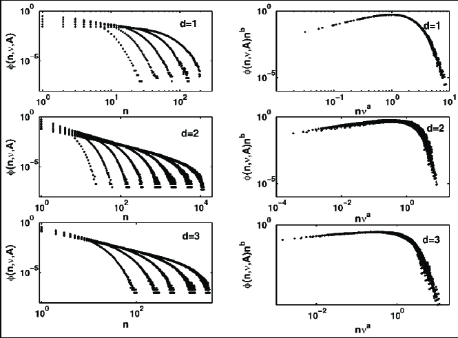
Figure 1: Left column: plots of the normalized RSA for $d=1,2,3$ with $\nu=0.001,0.003,0.01,0.03,0.1$ (the $d=2$ plot also shows the results for $\nu=0.0001,0.0003,0.3$); $L=200$. Right column: plots of the data collapse yielding a measure of the exponents $a$ and $b$ in Table 1.

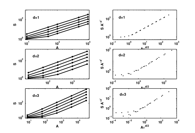
Figure 2: Left column: plots of the SAR for $d=1,2,3$ with $\nu=0.001,0.003,0.01,0.03,0.1$. Right column: plots of the data collapse yielding a measure of the exponent $z^{\prime}$ in Table 1.

Let us introduce a scaling form of the normalized RSA distribution of species, $\phi(n,\nu,A)\equiv f(n,\nu,A)/S(\nu,A)$, where $f(n,\nu,A)$ is the number of species with $n$ individuals:

$$\phi(n,\nu,A)=n^{-b}\hat{\phi}(n\nu^{a},A\nu^{d/2}),$$ (5)

where $b$ is an as yet undetermined exponent. By definition,

$$\sum_{n}\phi(n,\nu,A)\equiv 1$$ (6)

and

$$\sum_{n}n\phi(n,\nu,A)\equiv A/S(\nu,A)$$ (7)

(for simplicity, we set $\sigma=1$ so that $A=N$).

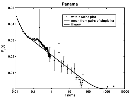
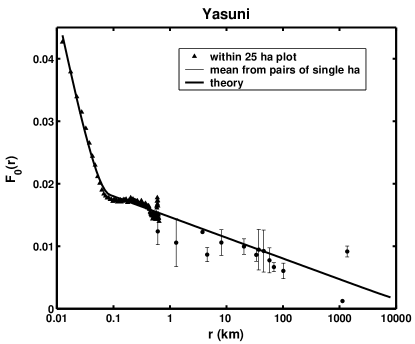
Figure 3: Beta Diversity data Condit et al. (2002) along with the best fits using Eq.(12) for plots in (a) Panama ($R=46$m, $\gamma_{0}^{-1}=68$m, $\gamma_{1}^{-1}=210$km and $c_{0}=0.012$) and in (b) Ecuador-Peru (Yasuni) ($R=86$m, $\gamma_{0}^{-1}=69$m, $\gamma_{1}^{-1}=23,500$km and $c_{0}=19$). The Janzen-Connell effect pushes conspecific individuals further away from each other and thus the probability function $F_{0}$ declines more steeply within the zone of its operation than at larger distances as in the data. Note that for length scales much bigger than $R$, in a regime in which Janzen-Connell effects do not play a significant role, the beta diversity curve decays much slower with length in Yasuni than in Panama by nearly a factor of $100$. This difference may be attributed to a very strong climatic gradient (in annual rainfall) across the isthmus in Panama, which causes rapid spatial changes in forest composition. In Yasuni, on the other hand, there are large areas with very similar climate. The experimental protocol and a description of the symbols are in Condit et al. (2002)

The normalization condition Eq.(6) becomes

$$1=\sum_{n\geqslant 1}\phi(n,\nu,A)\sim\nu^{a(b-1)}\int_{\nu^{a}}^{\infty}\mathrm{d}xx^{-b}\hat{\phi}(x,A\nu^{d/2}).$$ (8)

Assuming that $\hat{\phi}(x,y)$ does not diverge as $x$ tends to zero (which is justified a posteriori by numerical simulations), one finds that $b>1$ if $\hat{\phi}(x,y)$ approaches a constant value (modulo multiplicative logarithmic corrections) and $b=1$ if $\hat{\phi}(x,y)\rightarrow 0$ as $x\rightarrow 0$. In both cases $\hat{\phi}(0,y)$ is independent of $y$ (also in accord with the results of computer simulations). The condition on the average population per species, Eq.(7), leads to

$$\nu^{-d(1-z^{\prime})/2}\hat{S}^{\prime}(A\nu^{d/2})\equiv\sum_{n\geqslant 1}n\phi(n,\nu,A)$$ (9)

$$\sim\nu^{a(b-2)}\int_{\nu^{a}}^{\infty}\mathrm{d}xx^{1-b}\hat{\phi}(x,A\nu^{d/2}),$$

where $\hat{S}^{\prime}(y)=y^{1-z^{\prime}}/\hat{S}(y)$. Detailed simulations followed by a scaling collapse indicate that in all dimensions, $b<2$. It then follows that the lower integration limit in the above integral can be safely put to zero (a non-zero lower limit of integration would merely result in corrections to scaling) leading to the scaling relation

$$a(2-b)=\frac{d}{2}(1-z^{\prime})$$ (10)

and

$$\hat{S}^{\prime}(A\nu^{d/2})=\int_{0}^{\infty}\mathrm{d}xx^{1-b}\hat{\phi}(x,A\nu^{d/2}).$$ (11)

The linear dependence of $S(\nu,A)$ on $A$ arises from $\phi$ becoming independent of $A$ in the limit $A\gg\nu^{-d/2}$ (see Eq.(7)). This then leads to the scaling function $\hat{S}(y)\sim y^{1-z^{\prime}}$ in Eq.(7). This also follows from noting that $\hat{S}^{\prime}$ approaches a constant value for large $A$ (Eq.(9)).

We have carried out extensive simulations with hypercubic lattices of various sizes in $d=1,2,3$. A series of simulations with fixed size and varying speciation rate was used for the determination of the normalized RSA ($L=200$ for $d=2$ and $L=100$ for $d=1,3$, $L$ being the side of the hypercube used). Another series of simulations, varying both the speciation rate and $L$ was carried out to determine the SAR curves. $S(\nu,A)$ is the mean number of species in a simulation with speciation rate $\nu$ on a hypercubic lattice of size $A=L^{d}$. In order to carry out the collapse, we used the automated procedure described in Bhattacharjee and Seno (2001). Applying this procedure to the data on the normalized RSA obtained in our simulations, we were able to obtain the values of the exponents $a$ and $b$ (see Table 1, and Fig.1).

As expected, our extensive computer simulations indicate that $\phi$ is only weakly dependent on $A\nu^{d/2}$. In all dimensions the scaling exponents (see Table 1) approximately satisfy Eq.(10) and $b$ is in the interval $(1,2)$. Figure 2 shows a collapse plot which confirms the scaling postulates above. The biggest deviation from our theory is found in the value of $a$ in $d=2$, the upper critical dimension for diffusive processes and are suggestive of logarithmic corrections. Interestingly, our scaling relation seems to hold even for this case.

We conclude with a generalization of our model which provides an excellent quantitative fit to the $\beta$-diversity data of two tropical forests. The key idea is that the factor $\gamma$ in Eq.(2) can, in principle, take on two distinct values ($\gamma=\gamma_{0}$, $r<R$; $\gamma=\gamma_{1}$, $r\geqslant R$, where $R$ is a characteristic length scale separating the two distinct regimes). Such an effect arises physically from now well-established density-dependent processes first hypothesized by Janzen Janzen (1970) and Connell Connell (1971) in which the survival probability for an offspring is decreased in the vicinity of adults of the same species. Janzen and Connell postulated that this increased mortality rate of seeds and seedlings near adults arise from the presence of pests that are host-specific, i.e, specialized to that type of tree, and experimental evidence supports this conclusion Harms et al. (2000). The microscopic model that we consider is slightly modified from the previous version in that there is a non-zero probability that a new-born is immediately killed with a probability proportional to the number of conspecific adults within a circle of radius $R$ centered at the site.

The solution of Eq.(2) in $d=2$ with two distinct values of $\gamma$ is

$$F_{0}(r)=\left\{\begin{array}[]{cl}c_{0}K_{0}(\gamma_{0}r)+c_{1}I_{0}(\gamma_{0}r),&r<R\\ \\ c_{2}K_{0}(\gamma_{1}r),&r>R\end{array}\right.$$ (12)

where $I_{0}$ and $K_{0}$ are modified Bessel functions Abramowitz and Stegun (1965) and the constants $c_{1}$ and $c_{2}$ are fixed by imposing the continuity of $F_{0}(r)$ and its derivative at $r=R$ ($I_{0}(r)$ diverges as $r\rightarrow\infty$ and is therefore excluded in the region $r>R$). Figure 3 shows that our theory leads to good fits of the data on $\beta$-diversity for tree communities in both central Panama (top panel) and Ecuador-Peru Condit et al. (2002).