Identifying Biomagnetic Sources in the Brain by the Maximum Entropy Approach

Abstract

Magnetoencephalographic (MEG) measurements record magnetic fields generated from neurons while information is being processed in the brain. The inverse problem of identifying sources of biomagnetic fields and deducing their intensities from MEG measurements is ill-posed when the number of field detectors is far less than the number of sources. This problem is less severe if there is already a reasonable prior knowledge in the form of a distribution in the intensity of source activation. In this case the problem of identifying and deducing source intensities may be transformed to one of using the MEG data to update a prior distribution to a posterior distribution. Here we report on some work done using the maximum entropy method (ME) as an updating tool. Specifically, we propose an implementation of the ME method in cases when the prior contain almost no knowledge of source activation. Two examples are studied, in which part of motor cortex is activated with uniform and varying intensities, respectively.

1 Introduction

Magnetoencephalographic (MEG) measurements record magnetic fields generated from small currents in the neural system while information is being processed in the brain Hamalainen . In the classical cortical distributed model, the activation of neurons in the cortex is represented by sources of currents whose distribution approximates the cortex structure, and MEG measurements provide information on the current distribution for a specific brain function Hamalainen . In practice, given an set of current sources $J_{\beta}$, $\beta=\{1,\ldots,N\}$ and a set of magnetic field detectors labeled by $l=\{1,\ldots,d\}$, the relation between the field strengths $M_{l}$ measure by the detectors and the sources can be expressed as

$$M_{l}=\sum\nolimits_{\beta=1}^{N}A_{l}^{\beta}J_{\beta}+\chi;\qquad l=1,\ldots,d,\ \beta=1,\ldots,N.$$ (1)

where A is a $d\times N$ matrix whose elements $A_{l}^{\beta}$ are known functions of the geometric properties of the sources and the detectors, as determined by the Biot-Savart law Magnetic , and $\chi$ indicates noise, to be ignored here. The detail form of $A$ applicable to the present study is given in Bai03 . In tensor analysis notation Eq. (1) may be simply expressed as ${\bf M}={\bf A}\cdot{\bf J}$. In what follows, we adopt the convention of summing over repeated index ($\beta$ in Eq. (1)). In standard MEG Eq. (1) appears as an inverse problem: the measured field strengths M are given and the unknowns are J. Since the total number $d$ of detectors that can be deployed in a practical MEG measurement is far less than the number of current sources, the answer to Eq. (1) is not unique and the inverse problem is ill-posed Clarke88 ; Alavi93 .

A number of methods have been proposed to solve Eq. (1), including the least-square norm Hamalainen , the Bayesian approach Baillet01 ; Schmidt97 , and the maximum entropy approach Clarke88 ; Alavi93 ; Khosla97 ; He00 ; Besnerais99 ; Amblard04 . In the method of maximum entropy (ME) the MEG data, in the form of the constraints M - A$\cdot{\bf J}=0$, is used to obtain a posterior probability distribution for neuron current intensities from a given prior (distribution). In Amblard04 , the method is implemented by introducing a hidden variable denoting the grouping property of firing neurons. Here we develop an approach such that ME becomes a tool for updating the probability distribution ShoreJohnson ; JSkilling88 ; Caticha ; Tseng04 .

2 Computational detail

ME updating procedure. Let the set r to be current intensities $r_{\beta}$ caused by neuron activities in the cortex at sites $\beta=1,\ldots,N$, and $p_{\beta}(r_{\beta})$ be the probability current intensity distribution at site $\beta$. Assuming the N current sources to be uncorrelated, we define the joint probability distribution as $P({\bf r})=\prod_{\beta=1}^{N}p_{\beta}(r_{\beta})$. The current at site $\beta$ is then $J_{\beta}=\langle r_{\beta}\rangle=\int r_{\beta}P({\bf r})dr_{\beta}$. Suppose we have prior knowledge about neuron activities expressed in terms of the joint prior $u({\bf r})=\prod_{\beta=1}^{N}u_{\beta}(r_{\beta})$. The implication is that would produce currents J that does not satisfy Eq. (1) (here without noise). Our goal is to update from this prior to a posterior $P({\bf r})d{\bf r}$ that does satisfy Eq. (1). The ME method states that given $u({\bf r})$ and the MEG data, the preferred posterior $P({\bf r})d{\bf r}$ is the one that maximizes relative entropy $S[P,u]$,

$$S[P,\mu]=-\int d{\bf r}\mbox{ }P\left({\bf r}\right)\ln\left(P\left({\bf r}\right)/u\left({\bf r}\right)\right)$$ (2)

subject to constraints Eq. (1). Here $P({\bf r})$ is given by the variational method,

$$P({\bf r})d{\bf r}=Z^{-1}u({\bf r})\exp(-{\hat{\lambda}{\bf A}{\bf r}})d{\bf r},\quad Z=\int d{\bf r}\mbox{ }u({\bf r})\exp(-{\hat{\lambda}{\bf A}{\bf r}})\stackrel{{\scriptstyle\mathrm{def}}}{{=}}e^{-F},$$ (3)

where $\hat{\lambda}$ is a row vector of length $d$ whose $l^{\mbox{th}}$ element $\lambda^{l}$ is the Lagrangian multiplier that enforces the $l^{\mbox{th}}$ constraints in Eq. (1), ${\hat{\lambda}{\bf A}{\bf r}}=\lambda^{l}A_{l}^{\beta}\langle r_{\beta}\rangle$ and the last equality in Eq. (3)defines the quantity $F$. Because A is known, $P({\bf r})$ is determined by $u({\bf r})$ and the $\lambda$’s. The elements of $\lambda$ are the solutions $\lambda^{l}=\bar{\lambda}^{l}$ in

$$A_{l}^{\beta}\left.\langle r_{\beta}\rangle\right|_{\lambda^{l}=\bar{\lambda}^{l}}=\left.-\partial\ln Z/\partial\lambda^{l}\right|_{\lambda^{l}=\bar{\lambda}^{l}}=\left.\partial F/\partial\lambda^{l}\right|_{\lambda^{l}=\bar{\lambda}^{l}}=M_{l},\quad l=1,\ldots,d.$$ (4)

This is the primal-dual attainment equation derived in Besnerais99 . Because Eq. (4) is a non-linear equation in the $\lambda$’s, the search for the $\bar{\lambda}$’s is non-trivial.

A standard approach is by iteration, specifically by successive steps of updating $P({\bf r})$. To demonstrate this we simplify notation and write $\nu^{\beta}=\lambda^{l}A_{l}^{\beta}$, or simply $\hat{\nu}=\hat{\lambda}{\bf A}$. Expectation value of currents can then be calculated through $\langle r_{\beta}\rangle=-\partial\ln Z/\partial\nu^{\beta}$. The updating process may now start with $P_{[0]}=u({\bf r})$ and a set $\hat{\lambda}_{[0]}$ and proceed with

$$P_{[i]}\left(r\right)d{\bf r}={Z^{-1}_{[i]}}P_{[i-1]}(r)e^{-\hat{\nu}{\bf r}}d{\bf r},\quad Z_{[i]}=\int P_{[i-1]}(r)e^{-\hat{\nu}{\bf r}}d{\bf r},$$ (5)

where $[i=1,2,\cdots]$ denotes the $i^{\mbox{th}}$ updating step and $\nu=\hat{\lambda}_{[i-1]}A$. At each step $\hat{\lambda}_{[i-1]}$ is updated to $\hat{\lambda}_{[i]}$ according to Eq. (4). Formally the updating process converges at the solution of Eq. (4), which is a fix-point $\hat{\lambda}_{*}$ of Eq. (5): $\hat{\lambda}_{[i]}=\bar{\hat{\lambda}}=\hat{\lambda}_{*}$. Then the current intensities will be fix-points $\langle r_{\beta}\rangle_{*}$ such that ${\bf M}={\bf M}_{*}={\bf A}\langle{\bf r}\rangle_{*}$. In practice the fix-point may not be reached with infinite accuracy within finite time, and the updating may be terminated when the quantity

$$B_{mse}\stackrel{{\scriptstyle\mathrm{def}}}{{=}}-10~{}\ln\left({\left\|{\bf M}_{*}-{\bf M}\right\|}^{2}/\left\|{\bf M}\right\|^{2}\right)$$ (6)

attains a predetermined value. It is important to stress that unless the prior $u({\bf r})$ properly reflects sufficient knowledge about neuron activities, there is no guarantee that the fix-point $\langle{\bf r}\rangle_{*}$ is closely related to the actual current intensities.

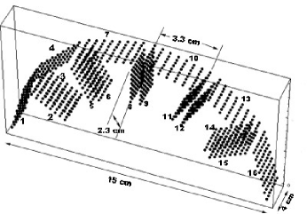
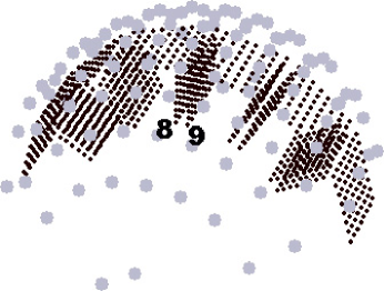
Figure 1: A (left panel): Distribution of current sources used in study. The motor cortex is represented by the patches 7 to 10. B (right panel): Distribution of magnetic field detectors on a hemisphere 2 cm from the scalp.

Sources with Gaussian distributed intensities. Pertinent general information on the geometric structure of the cortex and neuron activities, readily obtained from experiments such as functional magnetic resonance imaging (fMRI), positron emission tomography (PET), etc., is incorporated in a distributed model Baillet01 in which current sources, modeled by magnetic dipoles, are distributed in regions below the scalp. A schematic coarse-grained representation of this model is shown in Fig.1A, where 1024 dipoles are placed on 16 planar patches, 64 dipole to a patch. Eight of the which are parallel to the scalp and the other eight normal. Regardless of the orientation of the patch, all dipoles are normal to the cortical surface with the positive direction pointing away from the cortex.

Information contained in a prior may be qualitative instead of quantitative. Here, our prior will include the information that the activation resides in a part of the motor cortex that in Fig.1A is represented by the patches 8 and 9, and utilize this prior information by placing a higher concentration of field detectors in the area nearest to those in Fig.1B. There is additional information such as neuronal grouping property. We follow Amblard et al. Amblard04 and group dipoles into cortical regions $C_{k}$, $k=1,2,\ldots K$, each containing $n_{k}$ dipoles with the $n_{k}$’s satisfying $N=\sum_{k=1}^{K}n_{k}$. Associated with $C_{k}$ is a hidden variable $S_{k}$ that expresses regional activation status: $S_{k}$=1 denotes an “excitatory state”, or a state of out-going current; $S_{k}$=-1 denotes an “inhibitory state” (in-going current); $S_{k}$=0 denotes a “silent state” (no current). With this grouping, the prior $u({\bf r})$ reduces to a sum of probability distributions $u({\bf r},S)$ over all possible configurations of $S=\{S_{1},\cdots S_{K}\}$:

$$u({\bf r})d{\bf r}=\sum\nolimits_{S}u({\bf r},S)d{\bf r}=\sum\nolimits_{S}\mu({\bf r}|S)\pi(S)d{\bf r}=\prod\nolimits_{k=1}^{K}\sum\nolimits_{S_{k}}\mu({\bf r}_{k}|S_{k})\pi(S_{k})d{\bf r},$$ (7)

where ${\bf r}_{k}=\{r_{\eta}|\eta\in C_{k}\}$ specifies the current densities of the sources in $C_{k}$; $\mu({\bf r}_{k}|S_{k})=\prod_{\eta\in C_{k}}\mu(r_{\eta}|S_{k})$ is the conditional joint probability of the dipoles in $C_{k}$ being in state $S_{k}$ and having current densities ${\bf r}_{k}$; $\pi(S_{k})$ is the probability of the region $C_{k}$ being in activation state $S_{k}$. For $\mu({\bf r}_{k}|S_{k})$ we adopt a Gaussian distribution for activated states Clarke88 ; Alavi93 ; Amblard04 :

$$\mu({\bf r}_{k}|S_{k}\neq 0)=\prod_{\eta\in C_{k}}\frac{1}{\sqrt{4\pi\sigma}}\exp\left[-\frac{1}{2\sigma}(r_{\eta}-\rho_{\eta[0]})^{2}\right].$$ (8)

For simplicity, all current distributions have the same standard deviation $\sigma$. Current sources at different sites have different mean intensities $\rho_{i[0]}$ whose signs also indicate the state of activation: positive for excitation and negative for inhibition. For silent states we let $\mu({\bf r}_{k}|S_{k}=0)=\delta({\bf r}_{k})=\prod_{\eta\in C_{k}}\delta(r_{\eta})$. We also write $\pi(S_{k}\neq 0)=1-\pi(S_{k}=0)=\alpha_{k}$, where $0\leq\alpha_{k}\leq 1$. We thus have,

$$u_{G}({\bf r})=\prod\nolimits_{k=1}^{K}\sum\nolimits_{S_{k}}\mu({\bf r}_{k}|S_{k})\pi(S_{k})=\prod\nolimits_{k=1}^{K}\left[(1-\alpha_{k})\delta({\bf r}_{k})+\alpha_{k}\mu({\bf r}_{k}|S_{k}\neq 0)\right],$$ (9)

where the subscript denote Gaussian distribution. This form simplifies the computation significantly. At the $i^{\mbox{th}}$ iteration we have:

$$Z_{[i]}=\mbox{\ }\prod\nolimits_{k=1}^{K}\left(\prod\nolimits_{j=1}^{i-1}Z_{k[j]}\right)^{-1}\left[1-\hat{\alpha}_{k[i-1]}+\hat{\alpha}_{k[i-1]}\prod\nolimits_{j=1}^{i}\exp\left(F_{C_{k}\left[j\right]}\right)\right],$$ (10)

$$\langle r_{\eta}\rangle_{[i]}=\hat{\alpha}_{k[i]}\rho_{\eta[i]},\quad\rho_{\eta[i]}=\rho_{\eta[i-1]}-\sigma\nu_{\eta[i-1]},\quad(\eta\in S_{k}),$$ (11)

$$\hat{\alpha}_{k[i]}=\hat{\alpha}_{k[i-1]}\left(\hat{\alpha}_{k[i-1]}+\left(1-\hat{\alpha}_{k[i-1]}\right)\prod_{j=1}^{i}\exp\left(-\bar{F}_{C_{k}[j]}\right)\right)^{-1},$$ (12)

where $\hat{\alpha}_{k[0]}=\alpha_{k}$ and $\hat{\alpha}_{k[1]}=\alpha_{k[1]}$; $F_{C_{k}[i]}=\sum_{\eta\in C_{k}}(2\sigma)^{-1}\left[\left(\rho_{\eta[i]}\right)^{2}-\left(\rho_{\eta[i-1]}\right)^{2}\right]$.

In the absence of any other prior information we take $\alpha$ to be a random number (between zero and one), $|\rho_{\beta[0]}|$ to have a random value up to 20 nA, the maximum current intensity that can be generated in the brain, and $\sigma$ to be the mean of $|\rho_{\beta[0]}|$. However, the inverse problem being ill-posed, and since the prior contains no activation information, the above strategy produces poor results as expected.

Better priors by coarse graining. In the absence of prior information on activation pattern, one way to acquire some “prior” information from the MEG data itself is by coarse graining the current source. Coarse graining reduces the severity of the ill-posedness because the closer the number of current sources to the number of detectors, the less ill-posed the inverse problem. Within the framework of the ME procedure described above, coarse graining can be simply achieved by setting $\rho_{\eta}$ for all $\eta$ in a given region $C_{k}$ to be the same. Here we choose to take an intermediate step that disturbs the standard ME procedure even less, by replacing the second relation in Eq. (11) by

$$\rho_{\eta[i]}=\langle r_{\eta}\rangle_{[i-1]}-\sigma\bar{\nu}_{\eta[i-1]}.$$ (13)

Note that in Eq. (11) $\langle r_{\eta}\rangle=\alpha_{k}\rho_{\eta}$ depends on the probability $\alpha_{k}$ common to region $C_{k}$, whereas $\rho_{\eta}$ does not explicitly. By replacing $\rho_{\eta[i-1]}$ by $\langle r_{\eta}\rangle_{[i-1]}$ on the right hand side of Eq. (13), we force the updated $\rho_{\eta}$ in each iteration to be more similar (although not necessarily identical). In practice we only use this modified ME to get information on the activity pattern, rather than the intensity, of the sources. Let $\langle\bf r\rangle_{\rm c}$ be the current intensity set obtained after a convergence criterion set by requiring $B_{mse}\geq B_{mse}^{\{c\}}$ (Eq. (6)). We now define a better prior set of Gaussian means $\hat{\rho}_{\rm c}$, where, in units of nA,

$$\rho_{\beta\mbox{c}}=\left\{\begin{array}[]{c}{\rm sign}(\langle r_{\beta}\rangle_{\rm c})\ 20,\quad|\langle r_{\beta}\rangle_{\rm c}|>2,\\ 0,\qquad\qquad\qquad|\langle r_{\beta}\rangle_{\rm c}|\leq 2.\end{array}\right.$$ (14)

These quantities, together with the obtained probabilities $\hat{\alpha}_{k{\rm c}}$ for the regions $C_{k}$, define a prior probability $P^{\{c\}}(\bf r)$, which may then be fed into the standard ME procedure for computing $\langle{\bf r}\rangle$.

This procedure may be repeated by requiring $B_{mse}$ to be not less than a succession of threshold values, $B_{mse}^{\{c1\}}<B_{mse}^{\{c2\}}<B_{mse}^{\{c3\}}<\cdots$, such that a successive level of better priors $\hat{\rho}_{\rm c1}$, $\hat{\rho}_{\rm c2}$, $\hat{\rho}_{\rm c3}$, $\dots$, and $P^{\{c1\}}(\bf r)$, $P^{\{c2\}}(\bf r)$, $P^{\{c2\}}(\bf r)$, $\dots$, may be obtained. Eventually a point of diminishing return is reached. In this work we find the second level prior is qualitatively better than the first, and the third is not significantly better than the second.

3 Results

In the following two examples, the 1024 current courses are partitioned into 16 patches, eight (4 cm wide and 3.3 cm long) parallel and eight (4 cm wide and 2.3 cm deep) normal to the scalp (Fig.1A). On each patch lies a 8$\times$8 rectangular array of sources that are divided into 16 four-source groups; that is, $K$=256. The interstitial distances on the horizontal (vertical) patches are 0.57 and 0.47 cm (0.57 and 0.33 cm), respectively. The distance between the adjacent vertical patches are normally 0.55 cm, but the distance $d_{89}$ will be varied for testing, see below. The detectors are arranged in a hemisphere surrounding the scalp as indicated in Fig.1B. The matrix A of Eq. (1) is given in Bai03 . The ME procedure is insensitive to $\sigma$ in the range 5$<\sigma<$100. In the coarse graining procedure we set $B_{mse}^{\{c1\}}$=100 and $B_{mse}^{\{c2\}}$=150. As noted previously, coarse graining a third time did not produce meaningful improvement on the prior. In the two examples, artificial MEG data are generated by having the sources on patch have uniform and varied current intensities, respectively.

Uniform activation on patch 8. In this case the “actual” activity pattern is: the 64 sources on patch 8 each has a current of 10 nA, and all other sources are inactive (Fig.2A.). With the distance $d_{89}$ set to be 0.55 cm, the results in the first and second rounds of searching for a better prior, and in the final ME procedure proper are shown in Fig.2B. In the plots, $B_{mse}$ is the defined in Eq. (6) and $mse$ is defined as

$$mse=-10\ln\left(\left\|\langle{\bf r}\rangle_{[i]}-\langle{\bf r}\rangle\right\|^{2}/\left\|\langle{\bf r}\rangle\right\|^{2}\right),$$ (15)

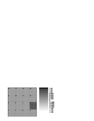
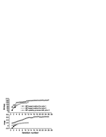
Figure 2: A (left panel): Contour plot indicates all 64 current sources on patch 8 are activated with an intensity of 10 nA. Gray scale on the right shows intensity level in units of 10 nA. Artificial MEG data M used in this section are generated through Eq. (1). B (right panel): $B_{mse}$ (top panel) and $mse$ (bottom panel) vs. iteration number.

where $\langle{\bf r}\rangle$ represents the actual source current intensity and the index $i$ indicates the iteration number. The solid triangles, squares, and crosses, respectively, give results from ME iteration procedures for constructing the first prior, second prior, and posterior. It is seen that $B_{mse}$ rises rapidly in the search for the first prior (solid triangles); four iterations were needed for $B_{mse}$ to reach 100. $B_{mse}$ is less than 100 at the beginning of the second prior search because the prior values for this search is not the posterior of the previous search, but is related to it by Eq. (14). The same goes with the the relation between the beginning of the ME proper (crosses) and the end of second prior search (squares). In the search for the second prior, $B_{mse}$ increases slowly after the seventh iteration, but eventually reaches 150 at the 12^th iteration. This already suggests that a round of search for a still better prior will not be profitable. In the ME procedure proper, $B_{mse}$ reaches 150 quickly at the fourth iteration, followed by a slow rise. After reaching 190 at the 14^th iteration the rise is very slow; the final value at the 26^th iteration is 195.

The dependence of the $mse$ value on the ME procedures and the iteration numbers essentially mirrors that of $B_{mse}$. The $mse$ for the final posterior is 68, which corresponds to an average of 3.3% error on the current intensities.

Resolving power as a function of $d_{89}$. We tested the resolving power of our ME procedure as a function of $d_{89}$. With uniform activation on patch 8, the computed $mse$ values versus $d_{89}$ are plotted in Fig.3A. The general trend is that $mse$ decreases with decreasing $d_{89}$ as expected: $mse=60\pm 10$ when $d_{89}>$0.044 cm; $mse$ drops sharply when $d_{89}$ is less than 0.04 cm; $mse$ is less than 8 when $d_{89}$ is less than 0.0044 cm. In the last instance the ME procedure loses its resolving power because the error on the current intensity is about 70%. On the other hand, $mse=60\pm 10$ implies an error of 5.6$\pm$2.6%. This means that if an error of no more than 8% is acceptable, the ME method should be applicable to a source array whose density is up to one hundred times higher than that used in the present study.

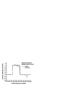
Figure 3: A (left panel): $mse$ value vs. the separation $d_{89}$ between patches 8 and 9. The distances $d_{89}$=0.55, 0.0275 and 0.0035 cm are marked out and labeled (1), (2) and (3), respectively. B (right panel): Reconstructed $\langle{\bf r}\rangle$ vs. source number for the cases (1) (solid line) and case (2) (dashed line) in A.

Resolving power as a function of depth. Signals from sources deeper in the cortex are in general weaker at the detectors and are harder to resolve. This effect is shown in Fig.3B. The abscissa gives the source numbers on patch 8 (449 to 512) and patch 9 (513 to 576). The sources are arranged in equally spaced rows of eight, such that 449-456 and 513-520 are just below the scalp, 457-464 and 521-528 are 0.328 cm from the scalp, and so on. Fig.3B shows that when $d_{89}$=0.55 cm (solid line), the ME procedure can resolve all sources (up to a maximum depth of 2.3 cm). This resolving power decreases with decreasing $d_{89}$. When $d_{89}$=0.0275 cm the ME procedure fails for sources at a depth of 2 cm or greater (that is, sources 496-512 and 561-576 on patches 8 and 9, respectively).

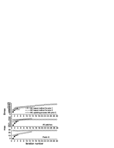
Figure 4: A (left panel): $Bmse$ and $mse$ values for the case of varied activation on patch 8 (see text). B (right panel): Reconstructed (dash line) and (artificially generated) actual (black line) $\langle{\bf r}\rangle$ $vs$. current source number on patches 8 and 9.

Varied activation on patch 8. We tested the ME procedure in a case with a slightly more complex activation pattern (still unknown to the prior): with $d_{89}$=0.55 cm, all current sources on patch 8 are activated, with those near the center of the patch having higher intensities than those in the peripheral. All other sources are silent. We used random source current densities as zeroth order prior, employed coarse graining twice, then used the standard ME to obtain the final reconstructed current intensities. With $d_{89}$=0.55 cm, the dependence of $Bmse$ and $mse$ on the iteration number is shown in Fig.4A. Interestingly for the ME procedure proper (crosses), only the $Bmse$ improves with iteration, whereas the $mse$ value remains a constant at about 18. This value is large compared to the value of 60$\pm$10 obtained for the case of uniform activation (Fig.2B). The solid and dashed lines in Fig.4B indicate the actual and reconstructed current intensities, respectively, for the sources on patches 8 and 9. These show that the poor result is caused by reconstructed false activation of sources 550 to 580 on patch 9. When sources other than those on patch 8 are forcibly forbidden to activate, $mse$ increases to 30 (bottom plot in Fig.4A), corresponding to a 22% error, suggesting that better results may be obtained when more reliable priors are given. This remains to be investigated.

Acknowledgments. This work is partially supported by grants NSC 93-2112-M-008-031 to HCL and NSC 94-2811-M-008-018 to CYT from National Science Council, ROC. We thank Jean-Marc Lina for his contribution during the early stages of this work.

References

- (1) M. Hämäläinen, R. Hari, R. J. LLmoniemi, J. Knuutila and O. V. Lounasmaa, Rev. Mod. Phys., 65, 413–497 (1993).
- (2) J. D. Jackson, “Classical electrodynamics” 2nd Ed. John Wiley & Sones, New York, 1990, pp.168–171; J. Sarvas, Phys. Med. Biol., 32, 11–12 (1987).
- (3) Hong-Yi Bai, “Detection of Biomagnetic Source by the the Method of Maximum Entropy”, master thesis, dept. of physics, National Central Univ. 2003 (unpublished).
- (4) S. Baillet and L. Garnero, IEEE Trans. Biomed. Eng., 44, 374–385 (1997); L. Gavit and S. Baillet, IEEE Trans. Biomed. Eng., 48, 1080–1087 (2001).
- (5) D. M. Schmidt, J. S. George and C. C. Wood, “Bayesian Inference Applied to the Electromagnetic Inverse Problem”, Los Alamos Natl. Laboratory report (http://stella.lanl.gov/bi.html), 1997, pp.1–12.
- (6) C. J. S. Clarke and B. S. Janday, Inverse Problems, 5, 483–500 (1989); C. J. S. Clarke, Inverse Problems, 5, 999–1012 (1989);
- (7) F. N. Alavi, J. G. Taylor and A. A. Ioannides, Inverse Problems, 9, 623–639 (1993).
- (8) D. Khosla and M. Singh, IEEE Trans. Nuclear Sci., 44, 1368–1374 (1997).
- (9) R. He, L. Rao, S. Liu, W. Yan, P. A. Narayana and H. Brauer, IEEE Trans. Magnetics, 36, 1741–1744 (2000).
- (10) G.L. Besnerais, J.-F. Bercher and G. Demoment, IEEE Tran. Inf. Theory, 45, 1565–1578 (1999).
- (11) C. Amblard, E. Lapalme and Jean-Marc Lina, IEEE Trans. Biomed. Eng., 51, 427–442 (2004). 106, 620–630 (1957).
- (12) J. E. Shore and R. W. Johnson, IEEE Trans. Inf. Theory, IT-26, 26–37 (1980); IEEE Trans. Inf. Theory, IT-27, 472–482 (1981).
- (13) J. Skilling, “The Axioms of Maximum Entropy” in Maximum Entropy and Bayesian Methods in Science and Engineering, ed. by G. J. Erickson and C. R. Smith, Kluwer, Dordrecht, 1988, pp.173–187; “Classic Maximum Entropy”, in Maximum Entropy and Bayesian Methods in Science and Engineering, edited. by J. Skilling, Kluwer, Dordrecht, 1989, pp. 45–52.
- (14) A. Caticha, “Relative Entropy and Inductive Inference” in Bayesian Inference and Maximum Entropy in Science and Engineering, ed. by G. Erickson and Y. Zhai, AIP Conf. Proc. 707, Am. Inst. Phys., New York, 2004, pp. 75–96.
- (15) C.-Y. Tseng and A. Caticha, “Maximum Entropy and the Variational Method in Statistical Mechanics: an Application to Simple Fluids” (under reviewing for Phys. Rev. E, 2004); “Maximum Entropy Approach to the Theory of Simple Fluids” in Bayesian Inference and Maximum Entropy in Science and Engineering, ed. by G. Erickson and Y. Zhai, AIP Conf. Proc. 707, Am. Inst. Phys., New York, 2004, pp. 17–29.