Reading Sequences of Interspike Intervals in Biological Neural Circuits

Abstract

Sensory systems pass information about an animal’s environment to higher nervous system units through sequences of action potentials. When these action potentials have essentially equivalent waveforms, all information is contained in the interspike intervals (ISIs) of the spike sequence. We address the question: How do neural circuits recognize and read these ISI sequences ?

Our answer is given in terms of a biologically inspired neural circuit that we construct using biologically realistic neurons. The essential ingredients of the ISI Reading Unit (IRU) are (i) a tunable time delay circuit modelled after one found in the anterior forebrain pathway of the birdsong system and (ii) a recently observed rule for inhibitory synaptic plasticity. We present a circuit that can both learn the ISIs of a training sequence using inhibitory synaptic plasticity and then recognize the same ISI sequence when it is presented on subsequent occasions. We investigate the ability of this IRU to learn in the presence of two kinds of noise: jitter in the time of each spike and random spikes occurring in the ideal spike sequence. We also discuss how the circuit can be detuned by removing the selected ISI sequence and replacing it by an ISI sequence with ISIs drawn from a probability distribution.

We have investigated realizations of the time delay circuit using Hodgkin-Huxley conductance based neurons connected by realistic excitatory and inhibitory synapses. Our models for the time delay circuit are tunable from about 10 ms to 100 ms allowing one to learn and recognize ISI sequences within that range of ISIs. ISIs down to a few ms and longer than 100 ms are possible with other intrinsic and synaptic currents in the component neurons.

I Introduction

Sensory systems transform environmental signals into a format composed of essentially identical action potentials. These are sent for further processing to other areas of a central nervous system. When the action potentials or spikes are comprised of identical waveforms all information about the environment is contained in the spike arrival times fano . The spike train can also be characterized in terms of interspike interval times for a given spiking sequence.

There are many examples of sensitive stimulus-response properties characterizing how neurons respond to specific stimuli. These include whisker-selective neural response in barrel cortex Welker ; Aara of rats and motion sensitive cells in the visual cortical areas of primates  Sugase ; Buracas .

One striking example is the selective auditory response of neurons in the songbird telencephalic nucleus HVC (proper name)  lewiiki ; Margoliash1 ; Margoliash2 ; Coleman1 . (Good introductions to the birdsong system may be found in the paper by Brenowitz, Margoliash, and Nordeen bren97 and the review by Brainard and Doupe brain02 .) Projection neurons within HVC fire sparse bursts of spikes when presented with auditory playback of the bird’s own song (BOS) and are quite unresponsive to other auditory inputs. The auditory nucleus NIf (interfacial nucleus of nidopallium), through which auditory signals reach HVC Janata ; Carr ; Coleman1 ; raskin , also strongly responds to BOS in addition to responding to a broad range of other auditory stimuli. NIf projects to HVC, and the similarity of NIf responses to auditory input and the subthreshold activity in HVC neurons suggests that NIf could be acting as a filter for BOS , preferentially passing that important signal on to HVC. It was these examples from birdsong that led us to address the ISI reading problem we consider here.

The representation of important neural information in ISI sequences suggests the presence of a biological neural network, perhaps widely used across species, capable of accurately recognizing specific ISI sequences. In this paper we develop such a network and demonstrate how biologically realistic neurons and synapses can be used to construct and train such a network to recognize specific ISI sequences. We call the resulting network an ISI Reading Unit (IRU).

Key to the functioning of an IRU are two biological processes:

1. a time delay unit which, on receiving a spike at time $t_{0}$, produces an output spike at time $t_{0}+\tau(R)$, where R is a dimensionless parameter characterizing synaptic strength that can be used to tune the time delay $\tau(R)$;

2. a method for tuning the time delays in the IRU $\tau(R)$ using synaptic plasticity of inhibitory synapses as observed recently Haas .

Time delay circuits, thought of primarily as an abstract idea rather than as a particular biological circuit realization, have been considered before Buono ; Mauk ; Ivry . An exception to the descriptive modelling of neural time telling processes is the work of Buonomano dean which studies a two neuron model which can be tuned to respond to time delays. Buonomano identifies synaptic changes as the tuning mechanism that might underlie detection of time intervals. His model relies on a balance between excitatory and inhibitory synaptic strengths. His construction might provide an alternative to the time delay unit structure we explore here, but we do not present an analysis of his results here.

As discussed by these authors circuits for telling time more or less divide into three categories:

• time delays along pieces of axon resulting in delays as short as a few microseconds and found in detection circuits for inter aural time differences knudsen ;

• time delays of order hours or days connected with circadian rhythms, and

• time delays of tens to hundreds of milliseconds associated with cortical and other neural processing.

Our realization of a time delay circuit addresses this third category using ideas from an observed neural circuit in the birdsong system.

In investigating time differences between signals propagating from the birdsong nucleus HVC directly to the pre-motor nucleus RA and the same signal propagating to RA around the neural loop known as the anterior forebrain pathway (AFP), Kimpo, Theunissen, and Doupe kimpo reported a remarkable precision of the time difference between these pathways of 50 $\pm$ 10 ms across many songbirds and many trials.

In investigating models of this phenomenon and its implications, along with excitatory synaptic plasticity at the HVC $\to$ RA junction (robust nucleus of acropallium) (see inset figure  3), we Abar1 constructed a circuit of neurons based on detailed electrophysiological measurements by Perkel and his colleagues perkel1 ; perkel2 , in each of the three nuclei of the AFP. This circuit demonstrated a tunable time delay adjusted by the strength of inhibition of synapse from the nucleus Area X to the nucleus DLM. The precise value of the time delay in the birdsong circuit was attributed to a fixed point in the overall dynamics including excitatory synaptic plasticity at the HVC $\to$ RA junction. This investigation suggested a general form of time delay circuit that could be tuned by changing the strength of an inhibitory synaptic connection. We develop that idea here.

Using these biologically motivated ingredients, we have built a simplified neural time-delay circuit and show here how it can be tuned to produce time delays within the range of about 10 ms to 100 ms or so. We demonstrate how to train such a circuit using given specific ISI sequences, and then show how the trained circuit robustly recognizes the desired ISI sequence. Recognition is implemented here using a detection circuit that fires an action potential when two input spikes arrive within a short temporal window of $\delta$ ms, (taken here to be 1 ms), and responds with subthreshold activity otherwise.

The overall IRU circuit made up of a subcircuit of time delay units operates by producing a replica of the given ISI sequence. It then uses inhibitory synaptic plasticity to adjust the delays in a sequence of time-delay sub circuits to match the ISIs in the input sequences within the resolution threshold of $\delta$ ms. Success in this matching is seen in the spiking activity of the detection circuit. The IRU circuit is thus a candidate for how biological networks can accurately select particular environmental signals, potentially usable for further processing for decision making and required functionality, by keying on the representation of environmental signals as a specific spike sequence.

We first discuss the construction of the time delay circuit beginning with the design of a smallest possible biologically feasible neural circuit consisting of two neurons and then explain the mechanism of the three neuron time delay circuit abstracted from the birdsong system. We then address the issue of training this delay circuit using synaptic plasticity of inhibitory synapses to detect an input ISI sequence. We then proceed to develop our full ISI Reading Unit (IRU) and show how it can be used to recognize a specific ISI sequence on which it has been trained. We show that the circuit can be trained robustly in two types of noisy environments: (1) When there is random jitter on the ISIs in the input sequence, and (2) when extra spikes are randomly inserted into the ISI sequence. The latter represents, in a realistic biological setting, the presence of other spikes associated with additional activity in the system as a whole. We also explore how an IRU can be detuned when presentation of the selected ISI sequence is replaced by a random ISI sequence.

II A Biological Time-Delay Circuit

A two neuron time delay circuit is motivated by construction of a single neuron model of type I  Ermen , that has property of being able to produce spikes at very low frequencies. It can be shown that  Izhi for neurons of type I, the frequency of spiking as function of constant input current $I_{IN}$, obeys the following relationship,

$$f=C\sqrt{I_{IN}-I_{0}}$$

, where $I_{0}$, is the spiking threshold and C is the scaling constant, which is function of model parameters. This frequency current relationship is characteristic of saddle node bifurcation of neuron to spiking regime, typically observed in Type 1 neurons. A neuron model developed by Traub  Traub consisting of transient sodium channels, delayed rectifier potassium channel and a leak channel, described by following set of dynamical equations, has frequency current relationship of Type I neuron behavior.

$$C_{M}\frac{dV_{I}(t)}{dt} = g_{Na}m(t)^{3}h(t)(V_{Na}-V_{I}(t))$$

$$+ g_{K}n(t)^{4}(V_{K}-V_{I}(t))+g_{L}(V_{L}-V_{I}(t))$$

$$+ I_{IN}$$

where $V_{I}$ is the membrane voltage of neuron. $C_{M}$, is the membrane capacitance, $g_{Na}$, $g_{K}$ and $g_{L}$ are maximal membrane conductance of the transient sodium channel, the delay rectifier potassium channel and the leak channel. $m(t)$ and $n(t)$ are the activation gating variables, which open up when membrane voltage increases and $h(t)$ represents the inactivation gating variable which closes on increasing membrane potential. $V_{Na}$, $V_{K}$ and $V_{L}$ represent the reversal potential for sodium, potassium and the leak channels respectively. The particular values for the parameters used in our equation are given in the appendix.

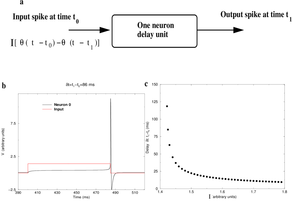
Figure 1: (a) Schematic of the one neuron delay unit model. Input to the neuron is a step current starting at time $t_{0}$ of the input spike and lasting until the first spike from the neuron. The intrinsic dynamics of the neuron to the spiking mode is through a saddle node bifurcation, typical of Type I neurons, that governs the delay produced by the neuron. (b) Scaled output from the delay unit, in response to step input current is shown. In this particular case, the neuron produces a delayed spike after about 87 ms. (c) Variation of the delay produced by the neuron as function of the strength of the input step current.

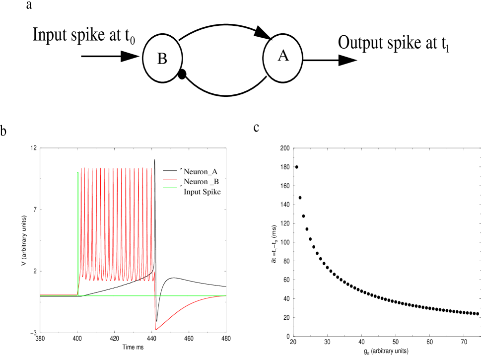
Figure 2: Schematic of a two neuron delay unit model. The input spike arrives at neuron B at time $t_{0}$, which pushes this bistable neuron into a spiking regime, raising the neuron A membrane voltage towards spiking threshold, until it eventually spikes. The spike from neuron A, pushes neuron B back into a stable resting state. (b) The membrane voltage of neuron A and neuron B, in response to an input spike at time $t_{0}=400$ ms. For this particular case, neuron A fires after a delay of around 42 ms. The delay produced is governed by the strength of the excitatory synaptic connection from neuron B to neuron A. (c) Plot of delay as a function of the strength of the excitatory synaptic input from neuron B to neuron A.

Using this neuron model, we construct a single neuron time delay circuit as shown in Figure  1a. The input to the neuron is $I\left[\Theta(t-t_{0})-\Theta(t-t_{1})\right]$, where $\Theta(x)=0$ when $x\leq 0$ and $\Theta(x)=1$ when $x>0$. $t_{0}$, is the time of an input spike to the neuron and $t_{1}$, is the time of first output spike out of the neuron. The period of spiking $T=(1000/f)$ ms, for type I neurons obeys $T=1000/C\sqrt{I_{IN}-I_{0}}$, i.e., $T\rightarrow\infty$, as $I_{IN}\rightarrow I_{0}$. Therefore, using such a type I neuron model, with step input current, for the duration of first spike, we can construct a timedelay unit to obtain various time delays as a function of strength of $I_{IN}$. In Figure  1a, we show the delay $\tau=t_{1}-t_{0}$, from this one neuron model as a function of $I_{IN}$. A biologically feasible smallest possible model for time delay with two neurons using an extension of above ideas from our one neuron model is shown in Figure  2a. The circuit is composed of two neurons, neuron B which exhibits the property of bistability, of coexistent resting state and spiking state, which is observed in many a neuron models  Guttman and neuron A, which is of type I as discussed above. The input to this delay circuit is a spike occurring at time $t_{0}$ . The output of the model is a single spike at time $t_{1}$ from neuron A, and thus $\tau=t_{1}-t_{0}$. This can be changed as a function of the maximal conductance of the excitatory synaptic connection from neuron B to neuron A. A single input spike into neuron B moves it into its spiking regime, providing enough depolarizing current into neuron A until it fires a spike. In order for spiking neuron B to provide enough depolarization to neuron A for it to eventually fire, the firing frequency of neuron B should be greater than the decay time of the excitatory synaptic connection from B to A. This necessitates the use of slow NMDA type excitatory synaptic connection from neuron B to A. A spike from neuron A, then provides a hyperpolarizing input to neuron B pushing it back into its rest state. In Figure  2c we show the plot of the time delay of this model as function of the maximal conductance of the excitatory synaptic input to neuron A from neuron B. An interesting feature of this two neuron time delay model is that, $\frac{d\tau}{dR}<0$. We will see in a later section on training the IRU to detect a given spike sequence, using observed learning rules of synaptic plasticity, the necessity of having $\frac{d\tau}{dR}>0$. This means that, the use of this two neuron unit delay model is infeasible for construction of IRU.

The simplest possible biologically feasible three neuron model for time delay circuit is motivated by the anterior forebrain pathway (AFP) loop in the song bird brain (Figure 3 inset). The AFP of songbirds is comprised of three nucles, the area X nucles, the DLM nucles and the lMAN nucles, each having a few times 10,000 neurons brain02 . The input to the AFP is via sparse burst of spikes from nucles HVC , entering via Area X, and the output signal of the AFP is from lMAN leaving the AFP to innervate the RA nucles. Within Area X two distinct neurons, spiny neurons (SN) and aspiny fast firing (AF) neurons, receive direct innervation from HVC perkel1 ; Perkelrecent . In the absence of signals from HVC, the SNs are at rest while the AF neurons are oscillating at about 20 Hz. The SNs inhibit the AF neurons, and these, in turn, inhibit neurons in DLM, a thalamic nucleus in the AFP Farries . The DLM neurons receiving this input from Area X are below threshold for action potential production while the AF neuron oscillates, but when the AF $\rightarrow$ DLM inhibition is released, the DLM neurons fire an action potential. This is propagated to lMAN, and then transmitted to RA. The time around this path differs from direct HVC $\rightarrow$ RA innervation by $50\pm 10\,$ ms  kimpo .

In our modelling of this observation Abar1 , treating each nucleus as a coherent action potential generating device, we found that LMAN played an unessential role in determining the time delay around the AFP while the strength of the AF $\rightarrow$ DLM inhibition could tune the time delay over a few tens of milliseconds.

From these observations, we have constructed a biologically feasible time delay circuit comprised of three neural units and two inhibitory synapses with a tunable synaptic strength.

The time delay circuit is displayed in Figure 3. Neuron A (similar to the SN in Area X) receives an excitatory input signal from some source. It is at rest when the source is quiet, and when activated it inhibits neuron B. Neuron B receives an excitatory input from the same source. It oscillates periodically when there is no input from the source. Neuron B inhibits neuron C. Neuron C produces periodic spiking in the absence of inhibition from neuron B.

In this paper each of the neurons A, B, and C is represented by a simple Hodgkin-Huxley (HH) conductance based model similar to the Traub model we discussed earlier with sodium, potassium, and leak currents as well as an injected DC current to set the spiking threshold. A more detailed neuron model for neuron C could include hyperpolarization activated $I_{h}$ channels and low threshold calcium $I_{T}$ channels, which facilitate post inhibitory rebound spikes Abar1 . Indeed, in the DLM neuron of the birdsong AFP this mechanism leads to calcium spikes as the output of “neuron C.”

When the inhibition from neuron B to neuron C is released by the signal from neuron A to neuron B, neuron C rebounds and produces an action potential some time later. This is due to its intrinsic stable spiking of neuron C in the absence of any inhibition from neuron B.

This time delay is dependent on the strength of the B$\rightarrow$C inhibition, as the stronger that is set the further below threshold neuron C is driven and the further it must rise in membrane voltage to reach the action potential threshold. This means the larger the B$\rightarrow$C inhibition, the longer the time delay produced by the circuit. Other parameters in the circuit, such as the membrane time constants, also set the scale of the overall time delay.

The direct excitation of neuron B by the signal source is critical. It serves to reset the phase of the neuron B oscillation, as a result of which the spike from neuron C is measured with respect to the input signal and thus makes the timing of the circuit precise relative to the arrival of the initiating spike. Absent this excitation to neuron B, the phase of its oscillation is uncorrelated with the arrival time of a signal from the source, and the time delay of the circuit varies over the period of oscillation of neuron B. This is not a desirable outcome, nor is it the way the AFP circuit appears to work.

We have constructed this circuit using standard Hodgkin-Huxley (HH) conductance based neurons and realistic synaptic connections. The dynamical equation for the three neurons shown in figure  3 are.

$$C_{M}\frac{dV_{i}(t)}{dt} = g_{Na}m(t,V_{i}(t))^{3}h(t,V_{i}(t))(V_{Na}-V_{i}(t))$$

$$+ g_{K}n(t,V_{i}(t))^{4}(V_{K}-V_{i}(t))+g_{L}(V_{L}-V_{i}(t))$$

$$+ g^{I}_{ij}S_{I}(t)(V_{revI}-V_{i}(t))+I^{syn}_{i}(t)+I^{DC}_{i},$$

where (i,j)=[A, B, C]. The membrane capacitance is $C_{M}$, and $V_{Na},V_{K},V_{L}$, and $V_{revI}$ are reversal potentials for the sodium, potassium, leak, and inhibitory synaptic connection respectively. $m(t),h(t)$, and $n(t)$ are the usual activation and inactivation dynamical variables; the equations for these are given in an appendix. $g_{Na},g_{K},g_{L}$ and $g_{E}$ are the maximal conductances of sodium, potassium and leak channels and excitatory connections respectively. $I^{DC}_{i}$ is the DC current into the A, B or C neuron. These are selected such that neuron A is resting at -63.74 mV in absence of any synaptic input, neuron B is spiking at around 20 Hz, and neuron C is also spiking at around 20 Hz, in absence of any synaptic inputs. $I^{syn}_{i}=g^{E}_{i}S_{E}(t)(V_{revE}-V_{i}(t))$ is the synaptic input to the delay circuit at neuron A and B, from the signal source at time $t_{0}$, where $g^{E}=(g_{EA},g_{EB},0)$. The inhibitory synaptic strengths, $g^{I}_{ij}$ in the delay circuit are $g_{BA}=R^{0}g_{I}$ and $g_{CB}=Rg_{I}$.

The dimensionless factors R and $R^{0}$, set the strength of $B\rightarrow C$ and $A\rightarrow B$ inhibitory connections respectively, relative to baseline strength $g_{I}$

$S_{E}(t)$ represents the fraction of neurotransmitter, docked on the postsynaptic cell receptors as a function of time. It varies between 0 and 1 and has two time constants: one for the docking time of the neurotransmitter and one for its release time. It satisfies the dynamical equation:

$$\frac{dS_{E}(t)}{dt} = \frac{S_{0}(V_{pre}(t))-S_{E}(t)}{\tau_{E}(S_{1E}-S_{0}(V_{pre}(t)))}.$$

The docking time constant for the neurotransmitter is $\tau_{E}(S_{1E}-1)$, while the undocking time is $\tau_{E}S_{1E}$. The function $S_{0}(V_{pre}(t))$, is 0 when $V_{pre}(t)=0$, representing no spike input from presynaptic terminal, and is 1 when $V_{pre}(t)>0$, representing spike input from the presynaptic terminal. For neurons A and B the presynaptic voltage is given by the incoming spike or burst of spikes arriving from some source at time $t_{0}$ (See figure  3). For our excitatory synapses we take $\tau_{E}=1\,$ms and $S_{1E}=1.5$, for a docking time of 0.5 ms and an undocking time of 1.5 ms. These times are characteristic of AMPA excitatory synapses.

Similarly $S_{I}(t)$ represents the percentage of neurotransmitter, docked on the postsynaptic cell as function of time. It satisfies the following equation

$$\frac{dS_{I}(t)}{dt} = \frac{S_{0}(V_{pre}(t))-S_{I}(t)}{\tau_{I}(S_{1I}-S_{0}(V_{pre}(t)))}$$

where we select $\tau_{I}=1.2\,$ ms and $S_{1I}=4.6$ for docking time of 4.32 ms and undocking time of 5.52 ms. The range of time delays produced by the three neuron delay circuit, depends on the docking and undocking times of this synapse. For the values given above we get the the delay curve as shown in figure  5. The inhibitory reversal potential $V_{revI}$ is chosen as -80mV. The voltage presynaptic to neuron B is $V_{A}(t)$ and when A spikes $V_{pre}(t)>0$ in the equation for $S_{I}(t)$ above.

The various parameters as well as the dynamical equations for the common activation and inactivation variables are presented in the appendix.

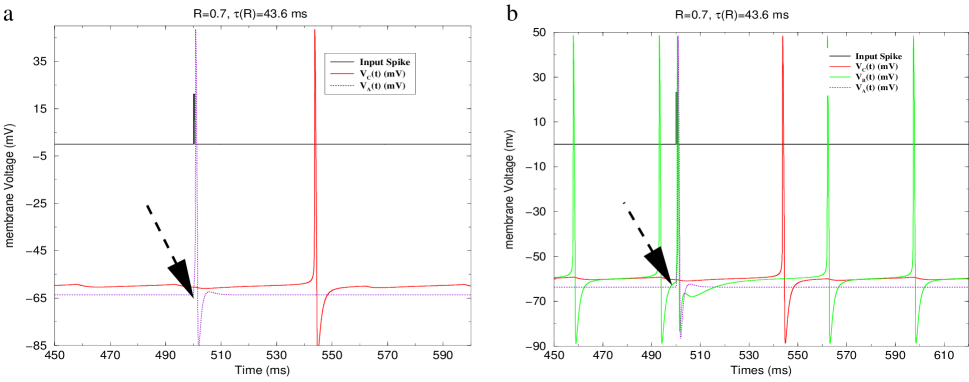
Figure 4: (a) For R = 0.7 we show the membrane voltages of neuron A (blue) and neuron C (red) in response to single spike input (black) arriving at neuron A and neuron B at time $t_{0}=500\,$ ms. For $R=0.7$ we see the output spike from neuron C occurring at $t=543.68\,$ ms, corresponding to $\tau(R)=43.6\,$ms. (b) For R =0.7 we again show the membrane voltages of neuron A (blue) and neuron C (red), and in addition now display the membrane voltage of neuron B (green). A single spike input (black) arrives at time $t=500$ ms. We see that the periodic action potential generation by neuron B is reset by the incoming signal. In Figures 2a and 2b the arrow indicates the time of the spike input to units A and B of our delay unit.

In Figures  4a and  4b we present examples of the response of the time delay circuit just described. In Figure  4 a single spike is presented to neurons A and B at $t_{0}=500.0\,$ms. For R = 0.7 the resulting time delay produced by the delay unit is 43.68 ms. In this figure we show the membrane voltage of neurons A and C. In Figure  4b we also show the membrane voltage of neuron B. It is clear in Figure  4b that the oscillations of neuron B are reset by the incoming signal, and the action potential generated at neuron C is a result of its internal dynamics, not of the period of oscillation of neuron B. The variation of the time delay with the strength of the B$\rightarrow$C inhibitory strength R is shown in Figure  5 for the particular set of parameters listed in the appendix. The important point here is that $\frac{d\tau(R)}{dR}>0$. For $R<R_{L}$, the inhibition on neuron C from neuron B, is not strong enough and the spike from neuron C is no longer correlated to input spike to the delay circuit. For $R>R_{U}$, the inhibition is so strong that neuron C does not produce rebound spike at all. As noted, one can, by changing the membrane capacitance and the strengths of the various maximal conductances and time course of inhibitory synaptic connections, place the variation of $\tau(R)$ near 10 ms or near 100 ms.

III An Interspike Interval Reading Unit (IRU)

Using these time delay units we now construct a circuit that can be trained to be selective for a chosen ISI sequence by repeated presentation of given ISI sequence. The main idea is that an ISI sequence starting at time $t_{0}$ and with spikes at times: $t_{0},t_{0}+T_{0},t_{0}+T_{0}+T_{1},\cdots,t_{0}+\sum_{j=0}^{N-1}T_{j}$ induces a replica of itself using time delay units with time delays $\tau_{0},\tau_{1},\cdots,\tau_{N-1}$. This replica sequence is compared to the original sequence and, if $|\sum_{j=0}^{i-1}(T_{j}-\tau_{j})|>\delta$ ms, where $\delta$ is the resolution of spike detection, then an inhibitory synaptic plasticity rule, as we discuss below, modulates delay unit $i$, so that this difference is reduced towards the tolerance limit of $\delta$ ms. When $|\sum_{j=0}^{i-1}(T_{j})-\tau_{j})|\leq\delta\,$ ms for each ISI in the training sequence, the IRU is considered trained. We choose $\delta=1$ ms, which reflects the width of actual action potentials; mathematically we could choose any $\delta>0$ as our convergence criterion (Appendix E). Training of the delay units in IRU is clearly a function of the learning rule implemented to adjust the $\tau_{i}$’s.

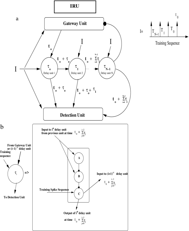
Figure 6: (a) Schematic diagram of an IRU. It is comprised of three parts, a gateway unit, a subcircuit of time delay units, and a detection unit. The gateway unit synchronizes the phase of the input ISI sequence with the action of the rest of the IRU and permits the first spike in the sequence to pass through and stimulate the sequence of time delay units. The gateway unit is turned off by inhibition until the last time delay units acts to restore it to its resting state. The time delay units create a replica of the ISI sequence, and the detection unit fires when two spikes within a small window, here 1 ms, are presented to it. (b) The abbreviated graphic for an individual time delay in the IRU shown in Figure 6a. The neurons A and B of each delay unit receive input from the previous delay unit. Depending on the strength of the inhibitory synapse from B$\rightarrow$C, a spike is produced by neuron C, after a certain delay. This is then sent to detection unit for comparison to the original ISI input and to the next delay unit to initiate its activity.

The complete circuit for an IRU is shown in Figure  6. The selected ISI sequence enters the “gateway” unit that passes on only the first spike. This effectively synchronizes the clocks of the first delay unit. The main purpose of this synchronization of the delay units is to prevent the other spikes in the input ISI sequence from interfering with the operation of these time delay units. The gateway unit is effectively closed after the first spike is received, and it is reset by an inhibitory signal sent by the last time delay unit when the replica ISI sequence has been created and passed on to the “detection” unit. The original ISI sequence is also passed directly to the time delay units for training and to the detection unit for comparison with the replica.

The gateway unit is shown in Figure  7. It is comprised of an excitatory neuron which receives the input ISI sequence and passes a first spike, at time $t_{0}$, on to the first time delay unit. It also excites a bistable inhibitory neuron or small neural circuit which moves into an oscillatory state and effectively turns the excitatory neuron off until it, in turn, is set back into its rest state by a signal from the last time delay unit.

The detection unit is comprised of a neuron (or small circuits of neurons) that fires when two spikes arrive within 1 ms of each other. It remains below its action potential threshold otherwise. There are many ways to accomplish this, and in the appendix we give an example of the detection unit we used in our construction of IRU.

Finally we need a mechanism to train each of the time delay units to adjust $|\sum_{j=0}^{i-1}(T_{j}-\tau_{j})|\leq 1\,$ ms. Equivalently we require a mechanism to adjust each delay unit such that $|T_{i-1}-\tau_{i-1}|=|\delta_{i-1}|\leq 1$ ms, for each of $i^{th}$ delay unit such that $|\sum_{j=0}^{i-1}\delta_{j}|\leq 1$ ms. This is done by presenting the target ISI sequence to the C-neuron of each time delay unit. The C-neuron of the i^th time delay unit fires an action potential at time $t_{0}+\sum_{j=0}^{i-1}\tau_{j}$ and receives a spike from the input ISI sequence at $t_{0}+\sum_{j=0}^{i-1}T_{j}$. If these are more than 1 ms apart, the inhibitory spike timing dependent plasticity rule will adjust it to be less than or equal to 1 ms as discussed in next section. There we discuss the experimentally observed spike timing dependent plasticity rule for an inhibitory synapse and explain how it plays a role in training the IRU to accurately detect the input ISI sequence.

IV IRU learning

A spike timing dependent plasticity rule for inhibitory synapses has recently been observed in layer II of entorhinal cortex by Haas, et al Haas . It gives the change in inhibitory synaptic conductance associated with the arrival of a spike at $t_{pre}$ at the presynaptic terminal and spiking of a postsynaptic neuron at $t_{post}$. As a function of $\Delta t=t_{post}-t_{pre}$, the change in synaptic conductance ${\Delta g_{I}(\Delta t)}$ normalized by the baseline synaptic conductance $g_{I0}$ is given by

$$\frac{\Delta g_{I}(\Delta t)}{g_{I0}}=\alpha^{\beta}\Delta t|\Delta t|^{\beta-1}\exp(-\alpha|\Delta t|).$$ (1)

An empirical fit to the data gives $\beta\alpha\approx 5$ to $10$ ms^-1. We have chosen $\beta=5$ and $\alpha=1\,$ ms ^-1 in the computations we report here (See the graphic inset in figure  8). This empirical learning rule allows tuning of the inhibitory synapse from B$\rightarrow$ C in the delay unit of the IRU. We identify $\Delta t$ as the time between the action potential generated at neuron C corresponding to $t_{pre}$, the time of C spike induced by presynaptic stimulation of neuron B and $t_{post}$, the time of receipt of the appropriate spike at neuron C, in the selected ISI sequence. For the first time delay unit, for example, this is $T_{0}-\tau_{0}(R_{0})$ (figure  6).

Consider the i^th delay unit and suppose the previous i-1 units have been adjusted such that $\left|\sum_{j=0}^{i-2}(T_{j}-\tau_{j})\right|\leq\delta$, where $\delta$ is the resolution scale for ISI detection. We now need to adjust the time difference $|\Delta t|=|T_{i-1}-\tau_{i-1}|$ between the ISI sequence time $t_{0}+\sum_{k=0}^{k=i-1}T_{k}$ and the present value of the time delay unit output at $t_{0}+\sum_{k=0}^{k=i-1}\tau_{k}$ for the i^th unit. Before any adjustment this $|\Delta t|$ is greater than $\delta$. As an example this is shown in Figure  8, for a scenario in which we start with the i^th delay unit initially tuned to produce a delay of $\approx$ 56.5 ms, and the target ISI it needs to detect is around 47.5 ms resulting in $|\Delta t|=9$ ms which is greater than $\delta$. $\delta$ $\approx 1\,$ ms.

The learning rule, shown in the inset of Figure 8, requires $g_{Ii}$, to be modified until $|\Delta t|<\delta$. If N represents the trial number of the repeated presentations of our desired ISI sequence, then we have a one dimensional map for the evolution of $g_{Ii}$, given by $g_{Ii}(N+1)=f(g_{Ii}(N))$, where $f(x)=x+\Delta x$. We are looking for a solution $g_{Ii}=g^{*}+\delta_{R}$, of the map corresponding to the resolution window $\delta$ for ISI detection. The case shown in Figure 8 corresponds to the situation when $\Delta t<-\delta$. The following analysis can easily be extended to the case when $\Delta t>\delta$.

The inhibitory synapse learning rule, for scenario shown in Figure  8 implies

$$\Delta g = \alpha^{\beta}\Delta t|\Delta t|^{\beta-1}\exp(-\alpha|\Delta t|)$$

$$= -(\alpha|\Delta t|)^{\beta}\exp((-\alpha|\Delta t|)),\left(\Delta t<-\delta<0\right)$$

$$< 0$$

where $\Delta t=T_{i}-\tau_{i}(g)$. Since $\Delta g<0$ implies the value of g over the next iteration decreases, and since $\frac{d\tau(g)}{dg}>0$ (Figure  5) implies the $\tau$ value decreases, this results in $\Delta t$ approaching zero from the right. As a result each repeated presentation of the desired ISI sequence will drive $g_{Ii}$ towards $g^{*}$.

It can be shown that for any learning rule $\Delta g(\Delta t)$, with $\tau(g)$, such that $\frac{d\tau}{dg}>0$ satisfying, the condition, $\Delta g>0\hskip 5.69046pt\forall\hskip 5.69046pt\Delta t>0$ and $\Delta g<0\hskip 5.69046pt\forall\hskip 5.69046pt\Delta t<0$, the convergence to desired ISI sequence will occur in finite number of steps (See appendix E ).

For the particular case of the learning curve used here, abstracted from empirical fit to observed experimental data on inhibitory synapses, the number of steps for convergence will depend on the criteria $\delta$ chosen for learning to stop. We give here several examples of learning for $\delta$ chosen to be 1 ms. In Figure  9, in particular, we show how the rate of convergence for learning changes as function of $\delta$, for IRU training on the ISI sequence $T_{i}$ to be 46.0 , 51.7 , 56.3 and 61.7 ms, respectively with the initial delays $\tau_{i}(N=0)$ for each of the delay units in IRU set at 52.68 ms, which is done by setting initial R value for each unit.

In Figure  10 we give an example of the training of an IRU with four time-delay units by a selected ISI sequence. The input ISI sequence is fed into the gateway unit which initializes activity in the delay unit. This ISI sequence also enters neuron C of each delay unit. In neuron C the ISI sequence participates in modulating the inhibitory synaptic strength of the B$\rightarrow$C synapse. At the same time the ISI sequence is also fed into the detection unit which detects the presence or absence of two spikes within our chosen resolution of 1 ms, thereby signaling detection of an input spike when there is a coincidence. In Figure  10 the ISIs in the training sequence, the $T_{i}$, are taken to be 50, 60, 55, and 58 ms respectively. The initial time delays $\tau_{i}(N=0)$ in the four time delay units are chosen to be 61.51, 57.55, 55.41 and 58.63 ms.

Since the IRU has time delay units connected in a chain, any modification in delay unit 1, for example, reflects itself in delay unit 2, and on down the chain. It is helpful to understand this connection among the delay units by expressing the way any given unit achieves its proper delay subtracting off the activity in earlier delay units. Figure  10 shows the time delays as a function of the number of presentations of the selected ISI sequence in three different forms. Figure  10a displays the error in all delay units (i=1 to 4)

$${\mathbf{E}^{IRU}_{i-1}}(N) = \sqrt{((t_{0}+\sum_{j=0}^{i-1}\tau_{j}(N))-(t_{0}+\sum_{j=0}^{i-1}T_{j}))^{2}}$$ (2)

$$= \sqrt{(\sum_{j=0}^{i-1}(\tau_{j}(N)-T_{j}))^{2}}.$$

as a function of the training sequence presentation number N. When the training is perfectly completed so $\left|\tau_{j}(N)-T_{j}\right|\approx 0$, for each of the delay unit this error goes to zero. The actual training continues until the error in each of the four delay units is within 1 ms of the threshold for spike detection by the detection unit.

In Figure  10b we plot the actual delay produced by the $i^{th}$ delay unit as it receives input spikes from the previous delay unit, (i-1)^st, at time $t_{0}+\sum_{j=0}^{i-2}\tau_{j}$ and produces spike output at time $t_{0}+\sum_{j=0}^{i-1}\tau_{j}$. In Figure  10c, we plot the difference

$${\mathbf{\Gamma}^{IRU}_{i-1}}(N) = (t_{0}+\sum_{j=0}^{i-1}\tau_{j}(N))-(t_{0}+\sum_{j=0}^{i-2}T_{j})$$ (3)

$$= \tau_{i-1}(N)+\sum_{j=0}^{i-2}(\tau_{j}(N)-T_{j})$$

corresponding to the evolution of the $i^{th}$ ISI in the IRU as a function of the training sequence presentation number. This quantity tells us how the value of the (i)^th time delay unit depends on the adjustments still taking place in the units earlier in the chain of delay units. When all the ISI’s have been detected, this number for each delay unit will be within $\delta$ ms of the actual ISI, as can be seen in Figure  10c. In the subsequent training examples, we only plot ${\mathbf{\Gamma}^{IRU}_{i-1}}(N)$, as shown in Figure  10c, and the corresponding error, ${\mathbf{E}^{IRU}_{i-1}}(N)$, as shown in Figure  10a.

The rate of change of the inhibitory synaptic conductance is determined by a scale factor of $g_{I0}$, set to $0.1e^{\beta}/\beta^{\beta}$ here, in the expression for $\Delta g_{I}(\Delta t)$. With this choice it takes about 88 presentations of the training ISI sequence to reach the desired accuracy for all time delays. In the simple training rule we use, changing the dimensionless number $g_{I0}$ from the value chosen above, to a large number increases the convergence rate as it simply scales time.

In Figure  11 we give an additional example of training an IRU in a noise free environment. We show in Figure  11 the results of training an IRU when all time delays are initially set to 52.13 ms, and the input ISI sequence has ISIs: 46, 51.7, 56.3, and 61.7 ms. Figure  11a shows the evolution of ISI from each delay unit as a function of the number of presentations of the selected ISI training set. In Figure  11b we show the detection unit time series in the untrained case, We see three subthreshold responses of the detection unit neurons associated with the input spikes, and we see one action potential associated with one of the untrained time delays having by chance been set within 1 ms of an input ISI. Figure  11c displays the detection unit output in a partially trained IRU when three ISIs in the time delay units lie within 1 ms of ISIs in the input ISI sequence. Finally in Figure  11d we show the fully trained IRU where we see four detection unit action potentials associated with the “coincidence,” within 1 ms, of the time delays and the ISIs in the time delay units.

V Performance of an IRU in a noisy environment

We have shown that an IRU is able to adjust its time delay units in a manner allowing detection of a specific noise free input ISI sequence. This is a “clean” environment allowing us to examine properties of IRU performance in absence of noise which is always present in any realistic biological setting. A thorough, systematic examination of IRU performance in a realistic noisy setting is the subject of another investigation. Here we confine ourselves to two instances of noise in the IRU detection.

In the first instance, we allow the training ISI sequence to have jitter on each of the ISIs in the sequence. This is the case where an input sensory signal which would ideally be represented by a fixed set of ISIs is now subject to noise in the neural circuitry or other environmental perturbations. The firing times of neurons in the processing circuitry transforming analog environmental signals to the ISI sequences would certainly contribute to this form of noise.

Figure  12a shows the training of the time delay units in an IRU in a noise free environment. In the top panel of Figure  12 we present the error in ISI detection ${\mathbf{E}^{IRU}_{i-1}}(N)$ at each delay unit in an IRU as a function of training number. In the bottom panel of Figure  12a we show the actual evolution of the ISI’s for each delay unit as a function of training number. The initial time delay for each unit is chosen to be $\tau_{i}(0)=52.68$ ms, and the ISI training sequence consists of the ISIs: $T_{1}=46.0$, $T_{2}=51.7$, $T_{3}=56.3$, and $T_{4}=61.7$ ms.

In Figure  12b we have introduced a jitter in each spike of the input ISI sequence uniformly distributing the spike time over $\pm 2$ ms around the mean values 46.0, 51.7, 56.3, and 61.7 ms. The IRUs train each delay unit until the time delay is within 1 ms of the input ISI. The training stops once the detection unit has produced 4 spikes corresponding to detection of each ISI. Since that might happen within $\pm$ 2 ms jitter of each spike, each of the output time delays in the bottom panel of Figure  12b is only reliable within the 2 ms jitter.

The process of repeatedly presenting the ISI sequence of interest to the IRU and altering the B$\to$C inhibition each iteration is dynamically a discrete time map of the IRU plus our $\Delta g_{I}$ rule. We are seeing in this example a representation of the stability of a fixed point of that iterated map system. This will appear again in our upcoming examples. We have not studied the basin of attraction of this fixed point or other long time dynamical behaviors of this map.

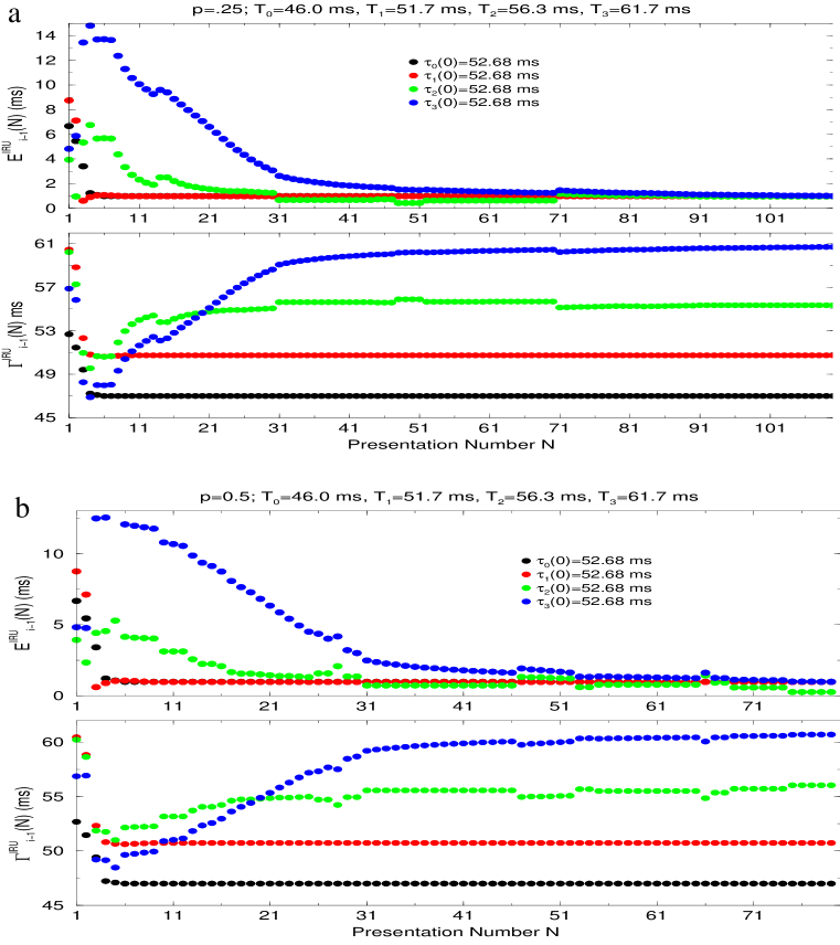
Figure 13: (a) Training the IRU on the deterministic ISI sequence 46, 51.7, 56.3, 61.7 ms in the presence of a random additional spike in the 3rd ISI with probability p= 0.25 (b) Training the IRU on the deterministic ISI sequence 46, 51.7, 56.3, 61.7 ms in the presence of a random additional spike in the 3rd ISI, with probability p= 0.5. In each case, the initial delays for each time delay unit (N=0) are set to 52.16 ms.

As a second instance of a noisy training environment, we have also investigated the situation in which an “extra” spike randomly appears in our deterministic ISI sequence. In Figures  13a and  13b we show two cases of learning the same underlying deterministic ISI sequence as in Figure  12 but now with an additional spurious spike present in the 3rd ISI interval with probability p=0.25 or p=0.5. We see that IRU is still able to learn the correct ISI sequence in about 101 presentations of the sequence with a random extra spike.

In terms of the possible existence of IRU in birdsong system, when the bird is deafened, the precise timing of the spikes resulting from sensory input is lost as it no longer receives auditory input, and as a result the song degenerates. In the context of an IRU this means that the IRU trained on the tutor song and maintained on the bird’s own song no longer receives the specific ISI sequence representing that song. Instead, in a manner we do not know precisely, it will receive random sequences of spikes with ISIs having little or nothing to do with birdsong but representing neural environmental noise.

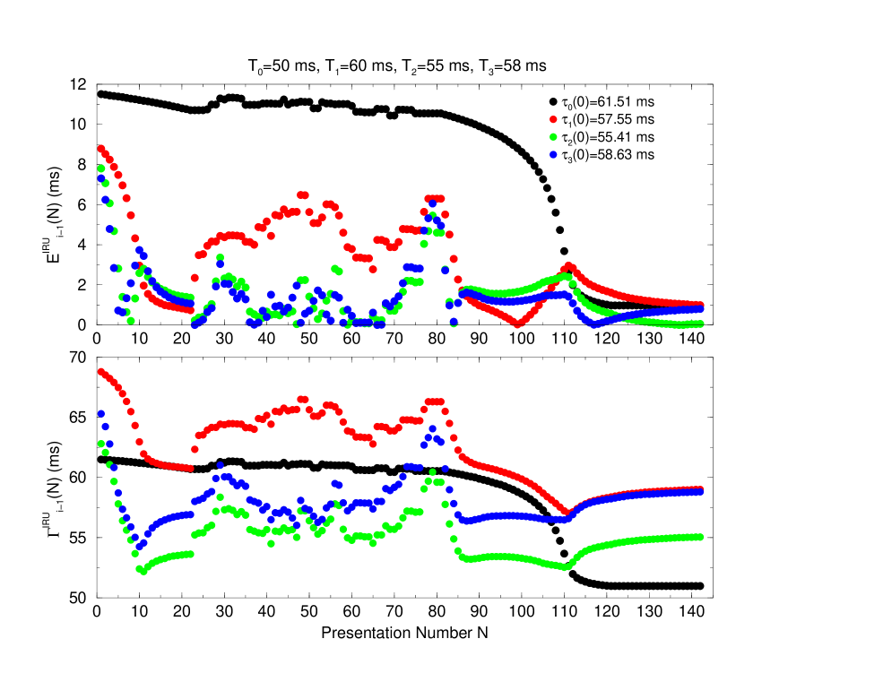
Figure 14: An IRU is initially trained on the sequence of ISIs: 50 ms, 60 ms, 55 ms, and 58 ms (as in Figure 7) for 20 presentations of the ISI sequence. Then the original sequence is replaced by an ISI sequence with the same mean values of the ISIs but with normally distributed noise of RMS variation 5 ms for 60 presentations. After this we make a further eighty presentations of the original noise free ISI sequence. As a conjecture we might connect the degeneration of the trained IRU in the presence of a noisy ISI sequence to the degeneration of song when a bird is deafened and no longer receives precise ISI sequences representing its own song at NIf or HVC.

In Figure  14 we show the training of an IRU for 20 presentations of the desired ISI sequence with ISIs of 50, 60, 55, and 58 ms. This is followed by 60 further presentations of a spike sequence with the same mean ISIs but perturbed by random normally distributed noise with zero mean and RMS variation of 5 ms. This is then followed by 60 presentations of the noise free initial ISI sequence. We see how the IRU is initially effectively training itself on the deterministic sequence, then it loses this connection with the desired ISIs when random spikes are received. Finally it recovers to train properly when the noise is removed.

VI Discussion

We have discussed a circuit composed of biologically motivated neurons and biologically motivated synaptic connections designed to respond selectively to a particular ISI sequence. We begin with the possibility of constructing a time delay circuit with the fewest possible number of neurons, two in this case, and then describe a three neuron time delay circuit model, abstracted from the birdsong system. The untrained IRU network has a set of time delay units constructed from three neurons each of which has an adjustable time delay set by the strength of an inhibitory synapse. These time delays are themselves set by a synaptic plasticity rule which compares the ISIs in the ISI sequence of interest to the time delays in the time delay units and adjusts the latter until they match the presented ISIs within a certain error, taken here to be 1 ms.

The construction of the overall circuit (an IRU) to read ISIs in the chosen sequence is quite general and is not solely connected with the observations which motivated its construction. It could be, though we do not have anatomical or electrophysiological evidence for this at this time, that such circuitry could be used generally to recognize the specific ISI sequences produced by sensory systems in response of environmental stimuli.

It seems clear that some circuit of this kind, whether or not it is the one we construct here, may well be utilized by animals for recognition of important sensory inputs. Those inputs are transformed by the sensory system into spike sequences, and in situation when all the spikes produced are identical, all the information is represented in the spike sequence. Reading those sequences in pre-motor or decision processing is required for various functional activities.

Our time delay circuit is constructed by analogy with one found in the AFP of the song system of songbirds. It is slightly simplified by the elimination of an output nucleus that is used for detailed tuning of the pre-motor responses in RA Kao , and it is represented by a three neuron circuit. Its instantiation in a biological system could, of course, use many more neurons as in the case of birdsong.

The time delay of this three neuron circuit is set in overall scale by the membrane capacitance of the neurons, and it is tuned in detail by the strength of one of the internal inhibitory connections. This strength is set by inhibitory synaptic plasticity using rules recently observed by Haas . The regime of operation of the IRU utilizing such time delay circuits, is governed by $\tau(R)$, and the IRU can train itself on ISIs in the interval $\left[\tau(R_{L}),\tau(R_{U})\right]$

We gave examples of the training of IRU network using an inhibitory synaptic plasticity rule. The outputs of the untrained network, a partially trained network, and a fully trained network which can recognize four ISIs are shown in Figures  11b-d. A “detection unit” which fires an action potential when a spike from a neuron C of the time delay unit arrives within 1 ms of a spike from the selected input ISI sequence produces no spikes for the untrained unit and reliably produces four spikes associated with the correct ISIs after training using synaptic plasticity. No spike in the detection unit is produced by the initial spike in the input ISI sequence; the detection unit responds only to correct ISIs after training using synaptic plasticity.

Our analysis does not address the response of an IRU to a desired ISI sequence when it is embedded in an environments with many extraneous spikes, and it does not address the reliability of the synaptic connections as a potential source of error in reading ISI sequences. For example, suppose the second spike in a sequence is missing because of failure of a synapse to fire when expected. How does the IRU performance degrade under such circumstances. It may be that the actual biological environments in which IRUs operate, assuming them to be present, require a statistical measure of detection efficacy. This would need to be carefully connected with the dramatic response of HVC neurons projecting to RA when stimulated by BOS as seen in the work of Coleman and Mooney Coleman1 . In connecting the ideas here about reading ISI sequences with models of the NIf and HVC nuclei in the avian birdsong system one will be able to address this and other issues in a quantitative fashion.

Appendix A Time Delay Unit of the IRU

In our three neuron model of the time-delay circuit we used HH conductance based models. In these equation there appear the sodium and potassium ion channels activation variables m(t) and n(t) and the sodium channels inactivation variable h(t). These satisfy, with $X(t)=\{m(t),h(t),n(t)\}$

$$\frac{dX(t)}{dt} = \alpha_{X}(V(t))(1-X(t))-\beta_{X}(V(t))X(t)$$

where V(t) here refers to the membrane voltage of the neuron, A, B, or C. We use, with V given in mV:

$$\alpha_{m}(V) = \frac{.32(13-(V-V_{th}))}{(\exp((13-(V-V_{th}))/4.)-1)}$$

$$\beta_{m}(V) = \frac{.28((V-V_{th})-40)}{(\exp(((V-V_{th})-40)/5)-1)}$$

$$\alpha_{h}(V) = .128\exp((17-(V-V_{th}))/18)$$

$$\beta_{h}(V) = 4.0/(1+\exp((40-(V-V_{th}))/5))$$

$$\alpha_{n}(V) = \frac{0.032(15-(V-V_{th}))}{(\exp((15-(V-V_{th}))/5)-1)}$$

$$\beta_{n}(V) = .5\exp((10-(V-V_{th}))/40)$$

and $V_{th}$=-65mV.

The various parameters chosen for the circuit are : The membrane capacitance is $C_{M}=1.0\frac{\mu F}{cm^{2}}$ . The maximal conductances,of the ionic currents in units of $mS/cm^{2}$ are, $g_{Na}=215,g_{K}=43,g_{L}=.813$. The reversal potentials in units of mV are $V_{Na}=50,V_{K}=-95,$ and $V_{L}=-64$. The excitatory synaptic conductances are $g_{EA}=1.0mS/cm^{2}$, $g_{EB}=1.0mS/cm^{2}$. The inhibitory synaptic conductance, $g_{I}=1mS/cm^{2}$. The scaling factor $R^{0}=50.0$ and $R$, varies as given in text. $V_{revE}=0\,mV$ , and $V_{revI}=-80\,mV$. $\tau_{E}=1.0\,ms$, $S_{1E}=1.5$, $\tau_{I}=1.2\,ms$, $S_{1I}=4.6$. The DC currents in the neurons are taken as $I^{DC}_{A}=0.0\mu A/cm^{2}$, $I^{DC}_{B}=1.97\mu A/cm^{2}$ and $I^{DC}_{C}=1.96\mu A/cm^{2}$

Appendix B The Gateway Unit

We model the gateway unit, as a bistable neuron coupled to standard HH model described above. The neuron A, receives the input ISI sequence beginning at time $t_{0}$. A spike from neuron A triggers the bistable neuron B, which is driven into a stable periodic spiking regime. Once the bistable neuron starts to fire, it, in turn, inhibits, neuron A and prevents it from responding any further to input ISI spikes. The membrane voltage of neuron A satisfies the following dynamical equation,

$$C_{M}\frac{dV_{A}(t)}{dt} = g_{Na}m(t)^{3}h(t)(V_{Na}-V_{A}(t))$$

$$+ g_{K}n(t)^{4}(V_{K}-V_{A}(t))+g_{L}(V_{L}-V_{A}(t))$$

$$+ g_{I0}S_{I}(t)(V_{revI}-V_{A}(t))$$

$$+ g_{E0}S_{E}(t)(V_{revE}-V_{A}(t))+I_{DC0}$$

where the symbols repeated from the description of the time delay unit have same meaning and values. In addition, the strength of inhibitory synapse from bistable neuron B onto A is $g_{I0}=100$ $mS/cm^{2}$ and the strength of excitatory synaptic input to neuron A from ISI sequence source $g_{E0}=1$ $mS/cm^{2}$. $I_{DC0}=1.0\,\frac{mA}{cm^{2}}$, such that neuron is sitting at resting potential of -63 mV.

The dynamics of neuron B which is in a bistable regime is given by

$$C_{M}\frac{dV_{B}(t)}{dt} = g_{Na}m_{\infty}(t)(V_{Na}-V_{B}(t))$$

$$+ g_{K}n(t)(V_{K}-V_{B}(t))+g_{L}(V_{L}-V_{B}(t))$$

$$+ I_{syn}(t)+I_{DC1}$$

where the gating variables $X(t)=\{n(t),m(t)\}$ satisfies the following kinetic equation,

$$\frac{dX(t)}{dt} = \frac{X_{\infty}(V(t))-X(t)}{\tau_{X}}$$

and the activation function, $X_{\infty}(V)=\{m_{\infty}(V),n_{\infty}(V)\}$, has the following functional dependence on voltage V,

$$X_{\infty}(V)=1/(1+\exp((V_{X}-V)/k_{X}))$$

$I_{syn}(t)$ is the excitatory synaptic current from neuron A on to neuron B, which is taken to be, $I_{syn}(t)=g_{E1}S_{E}(t)(V_{revE}-V_{B}(t))$, which represents AMPA type excitatory synaptic current. Finally $S_{E}(t)$ is taken to satisfy the following first order kinetic equation,

$$\frac{dS_{E}(t)}{dt} = \frac{S_{0}(V_{pre}(t))-S_{E}(t)}{\tau_{E}(S_{1E}-S_{0}(V_{pre}(t)))}.$$

where as described in the main text we have $\tau_{E}=1$ ms and $S_{1E}=0.5$, giving the docking time of .5 ms and undocking time of 1.5 ms. Finally, the various parameters appearing in these equations are $C_{M}=1\frac{\mu F}{cm^{2}}$; $g_{Na}=20,g_{K}=10,g_{L}=8.0$, in units of $mS/cm^{2}$; $V_{Na}=60,V_{K}=-90,$ and $V_{L}=-80$, in units of mV; $V_{m}=-20$mV, $k_{m}=15$, $V_{n}=-25$mV, $k_{n}=5$, $\tau_{n}=1\,$ms. The conductance of the excitatory synaptic connection is $g_{E1}=1\,mS/cm^{2}$. $I_{DC1}=4\,mA/cm^{2}$, such that the neuron B is at resting potential of around -62 mV.

Appendix C One and Two neuron Delay Circuit

All the parameters for one neuron model described in the main article are same as the ones used for construction of neural units for three neuron model as described in appendix A. For the two neuron model the bistable neuron B, satisfies the same set of dynamical equations as presented above for the bistable neuron B of the gateway unit. Similarly the type I neuron of the two neuron delay model shares same set of equations as described for the neuron A of the gateway unit. All the dynamical equations for the type 1 neuron and the bistable neuron described in the gateway section are same for description of the two neuron model, except for the excitatory synapse, which is modelled as NMDA type excitatory synapse, necessitated by the slow decay times, required for neuron B to provided enough excitatory input to neuron A for it to spike. The excitatory synaptic current from $B\rightarrow A$, is given by $I(t)=g_{E}S_{E}(t)B(V(t))(V_{revE}-V(t))$, where $B(V(t))=1.0/(1+0.288[Mg^{2+}]\exp(-0.062V(t)))$ and $[Mg^{2+}]=1$mM. The strength of inhibitory connection from neuron A to neuron B is 1 mS/cm² and the strength of excitatory synaptic input from source onto neuron B at time $t_{0}$ is 0.1 mS/cm².

Appendix D Detection Unit

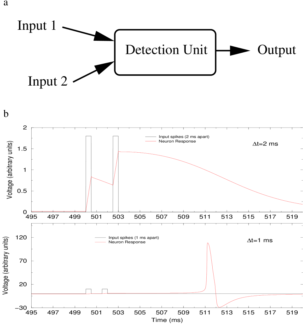
Figure 15: (a) Schematic of the detection unit. It receives two input spikes at various time delays. It responds with a spike if the two inputs are within 1 ms of each other. (b) Top panel The scaled response of the detection unit when two input arrive within 2 ms of each other. We see that the integrated input arriving at this delay does not result in neuron spiking. In the bottom panel we show the scaled neuron response to two input spikes arriving within 1 ms of each other. The detection unit produces a spike output, indicating coincidence detection.

The detection unit model used in our IRU, is a type I neuron model as discussed above for the delay unit in appendix A. It is tuned to respond to two input spikes arriving within a millisecond of each other. In Figure  15b top panel, we show the response of the detection unit when it receives two input spikes, 2 ms apart. The total integrated input at given time delay between these two inputs is not sufficient to push the neuron beyond its spiking threshold and the neuron responds only with an EPSP. However, when two input spikes, are sufficiently close in time, here within 1ms, as shown in Figure  15b bottom panel, the total integrated input is sufficient to push the neuron above its spiking threshold. Now it responds with a spike after a time delay of around 10 ms, governed by the integration time constant of the neuron dynamics.

Appendix E Linear Map for Learning Rule

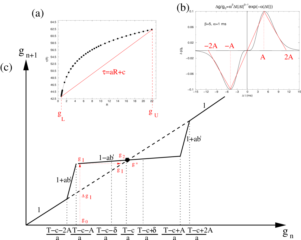
Figure 16: (a) Linear approximation for the delay produced by individual delay unit as function of inhibitory synaptic strength (b) Linear approximation of the learning rule observed for inhibitory synapse in entorhinal cortex. (c) The linearmap for evolution of inhibitory synaptic strength is depicted. Sample trajectory for evolution of the inhibitory synaptic strength following the linear learning rule is shown in red.

In this section we consider an approximation of the learning rule for evolution of inhibitory synapse, and the delay produced by each delay unit as function of strength of inhibitory connection from $B\rightarrow C$, as shown in Figure  16a and  16b, and compute an analytical expression for number of training sequence steps required for delay unit to detect a spike within $\delta$ ms resolution of actual ISI. The approximation shown in Figure 16a and  16b results in the following,

$$\frac{\Delta g_{I}}{g_{I_{0}}} = b\Delta t,\hskip 5.69046pt(|\Delta t|\leq A)$$

$$= -b\Delta t+2Ab,\hskip 5.69046pt(A<|\Delta t|\leq 2A)$$

$$= 0,\hskip 5.69046pt(|\Delta t|>2A)$$

with, $\tau=ag_{I}+c\hskip 5.69046pt(g_{L}\leq g_{I}\leq g_{U})$ and $\tau=0\hskip 5.69046pt(g_{I}<g_{L})$ and $\tau=\tau(g_{U})\hskip 5.69046pt(g_{I}>g_{U})$. The fact that $\Delta g=0$ for $|\Delta t|>2A$ implies that, learning will occur only for $\Delta t$ in the range of $\pm$ 2A ms, or in the map $f(g_{I}(N))$ the allowed variation in $g_{I}(N)$ is from (T-c-2A)/a to (T-c+2A)/a. Depending on the initial inhibitory synaptic strength of $g_{I}(0)=g_{0}$, with above linear learning rule, the number of steps for the delay unit to set its delay output within $\delta$ ms of actual ISI time that it needs to detect, $N(\delta)$, can be obtained as follows,

The trivial case of initial condition being within the $\delta$ window of actual ISI, results in $N(\delta)=0$. In the situation when $|\Delta t|\leq A$, the number of training iterations required for learning, is given by $N(\delta)=1+n_{1}$, where $n_{1}$, can be computed as follows. We begin in the region $\Delta t=T-\tau_{0}\leq A$, which corresponds to initial inhibitory synaptic strength lying in the interval,$(T-c-A)/a\leq g_{I}(0)\leq(T-c-\delta)/a$. At each iteration step i, as shown in the example path in Figure 16c, $g(i)$, increments by amount, $\Delta g_{I}(i)/(1-ab^{{}^{\prime}})$, where $b^{{}^{\prime}}=bg_{I_{0}}$. The total number of integer steps required for $g_{I}(0)=g_{0}$, to evolve to within $\delta$ ms window of T, is then given by

$$n_{1} = \left[\frac{\log\left(\frac{\delta}{(|T-\tau_{0}|)}\right)}{\log(1-ab^{{}^{\prime}})}\right]$$

where $\tau_{0}=ag_{0}+c$ and $[x]$, is the largest integer less than or equal to $x\in\mathbb{R}$.

It is important to note the factor of $b^{{}^{\prime}}$ appearing in the denominator of above equation. In the scheme of learning rule we have used in the main calculations, as $\Delta t\rightarrow 0$, $b^{{}^{\prime}}$, which represents the slope of the learning curve

approaches 0, and as we can see from above, theoretically the exact convergence of learning, i.e., $\Delta t=0$ requires, infinity of training steps.

In situation when the initial condition is such that $A<|\Delta t|<2A$, the number of training iterations required is given by $N(\delta)=2+n_{1}+n_{2}$, where

$$n_{1} = \left[\frac{\log\left(\frac{A}{|2A+\tau_{0}-T|}\right)}{\log(1+ab^{{}^{\prime}})}\right]$$

$$n_{2} = \left[\frac{\log\left(\frac{\delta}{|(T-c)-a\widetilde{g}|}\right)}{\log(1-ab^{{}^{\prime}})}\right]$$

$$\widetilde{g} = g_{0}{(1+ab^{{}^{\prime}})}^{n_{1}+1}+\frac{\left((1+ab^{{}^{\prime}})^{n_{1}+1}-1)(2A-(T-c)\right)}{a}$$

Linear fit to the learning rule used in the main text, which is abstracted from empirical fit to entorhinal cortex data, gives, $A=5$ms, $b^{{}^{\prime}}=0.02$ms^-1 and linear $\tau(g)$ curve implies, $a=0.9$ ms $c=42.58$ ms, $g_{L}=.75$ and $g_{U}=22.0$. In this approximation the maximum number of steps will correspond to beginning with $\Delta t$ error of $\pm 2A=10ms$. For a particular case of T=60 ms, and beginning with $\tau_{0}=51ms$, giving $\Delta t=9ms$, and taking $\delta=1ms$, solving the above equation gives, N=179, as total number of training cycles for the delay unit to learn.

Figures

Figure 3: Schematic diagram of the time-delay unit used in the IRU circuit. This is abstracted from a time delay network in the anterior forebrain pathway of the birdsong system as shown in the inset above. Th einset shows the AFP loop (Area X, DLM and lMAN) from the birdsong system that suggested our three neuron timedelay unit. Absent any input spikes, neuron A is at rest, neuron B oscillates periodically, and neuron C oscillates around its rest potential driven by periodic inhibitory input from neuron B. When an input spike arrives at neuron A and at neuron B at time $t_{0}$, neuron A fires an action potential and neuron B has the phase of its oscillation reset to be in synchrony with the time of arrival $t_{0}$ of the spike. The action potential in neuron A inhibits neuron B, and this releases neuron C to rise to its spiking threshold a time $\tau(R)$ later. R is the dimensionless scale of the $B\to C$ inhibition. Within a broad range for R, neuron C will fire a single spike at a time $t_{0}+\tau(R)$. The value of the conductance for the B $\to$ C inhibitory synapse is $g_{I}=Rg_{I0}$, with $g_{I0}$ a baseline conductance..

Figure 5: The delay $\tau(R)$ produced by the time delay unit as a function of $R$, the strength of the inhibitory synaptic connection $B\rightarrow C$. All other parameters of the time delay circuit are fixed to values given in the appendix. For $R<R_{L}$ the inhibition is too weak to control the precise spiking of neuron C, locked in with respect to signal input spike to the delay unit. For $R>R_{U}$ the inhibitory synapse is so strong that the neuron does not produce any action potential, effectively the delay out of the network is infinity.

Figure 7: Schematic diagram of the gateway unit for spikes entering the IRU. The function of this unit is to initiate the delay network activity by passing the first spike of input training sequence to the delay network, such that the activity of delay network is synchronized to that of the first spike of input training sequence and shutting off further spikes until it is reset by a signal from the last time delay unit in the IRU.

Figure 8: IRU learning: This is an example showing how the inhibitory synaptic mechanism plays a role in modulating the synaptic strength of the B$\rightarrow$C synapse of a given delay unit in the IRU. The insert shows the inhibitory plasticity rule we use in this paper Haas .

Figure 9: Convergence rate of learning of IRU, as function of the resolution scale $\delta$ for Detection unit to recognise ISI in the incoming spike sequence is plotted for a particular case of noise free ISI sequence of 46,51.7,56.5 and 61.7 ms , with initial delays for each delay unit being set at $\tau_{i}(0)=52.68$

Figure 10: Training an IRU to a desired ISI sequence consisting of 4 ISIs at $50,60,55,$ and $58$ ms.(a) The error in detection of ISIs as function of trial presentation number. The training continues until the error in detection of each ISI is within 1 ms, the resolution threshold for the detection unit. (b) The actual delay produced by each delay unit as learning modulates the inhibitory synaptic strength of the B$\rightarrow$C connection in each delay unit is plotted as function of training number N. (c) The ISIs produced by each delay unit of the IRU.

Figure 11: (a) Training of an IRU on the ISI sequence, $46,51.7,56.3,61.7$ ms when all time delays are initially (N=0) set to 52.13 ms. (b) Output of the detection unit when training begins. For the selected initial conditions, the detection unit is able to detect the 2nd ISI correctly at the beginning of training. This is a coincidence of our choice of initial conditions. The other ISIs are not yet trained and subthreshold EPSPs are activated in the detection unit. (c) Output of the detection unit in the middle of training. At this stage three of the ISIs in the selected ISI sequence have been matched by the IRU. (d) Output of the detection unit at the end of training when all ISIs in the input sequence have been matched in the IRU. In each of figures 8a, 8b and 8c, the red trace is the input training spike sequence.

Figure 12: (a) Deterministic ISIs. In the top panel, the error in the detection of the input ISI sequence for each delay unit is shown. In the bottom panel, we show how the delays of each time delay unit are modified with training to detect the ISI sequence consisting of 4 ISIs: $46.0,51.7,56.3$ and $61.7$ ms. (b) ISIs with jitter. We present the same ISI sequence, but with a jitter of $\pm\,$2 ms around the mean ISIs. In the top panel we again present the evolution of error in ISI detection in each delay unit. We see that it, in fact, takes fewer training sequence iterations than in the jitter free case, and, overall, the learning in the presence of this level of noise proceeds nearly as efficiently as in the deterministic scenario of Figure 9a. In the bottom panel the evolution in the presence of jitter of time delays from the delay units with learning is presented.

References

- (1) Fano, Robert M., Transmission of information; a statistical theory of communications, New York, M.I.T. Press (1961)
- (2) Welker, C., “Receptive fields of barrels in the somatosensory neocortex of the rat,” J Comp Neurol., 166, 173-89, (1976).
- (3) Aarabzadeh, E., S. Panzeri, and M. E. Diamond, “Whisker Vibration Information Carried by Rat Barrel Cortex Neurons,” J. Neurosci., 24, 6011-6020, (2004).
- (4) Sugase, Y., S. Yamane, S. Ueno, and K. Kawano, “Global and fine information coded by single neurons in the temporal visual cortex,” Nature, 400, 869-873, (1999).
- (5) Buracas, G.T., Zador A. M., DeWeese M.R., Albright T.D. , “Efficient Discrimination of temporal patterns by motion sensitive neurons in primate visual cortex,” Neuron, 9, 59-69, (1998).
- (6) Lewicki, M. and B. Arthur, “Hierachical organization of auditory context sensitivity,” J. Neurosci., 16, 6897-6998, (1996).
- (7) Margoliash, D., “Acoustic parameters underlying the responses of song-specific neurons in the white-crowned sparrow,” J Neurosci., 3, 1039-57, (1983).
- (8) Margoliash, D., “Preference for autogenous song by auditory neurons in a song system nucleus of the white-crowned sparrow,” J Neurosci. 6, 1643-61, (1986).
- (9) Coleman, M. and R. Mooney, “Synaptic Transformations Underlying Highly Selective Auditory Representations of Learned Birdsong,” J. Neurosci., 24, 7251-7265, (2004).
- (10) Brenowitz, E. A., D. Margoliash, and K. W. Nordeen, “An introduction to birdsong and the avian song system,” J Neurobiol. 33, 495-500, (1997).
- (11) Brainard, M. S, and A. J. Doupe, “What songbirds teach us about learning,” Nature, 417, 351-358, (2002).
- (12) Janata, P and D. Margoliash, “Gradual Emergence of song selectivity in sensorimotor structures of the male zebra finch song system,” J. Neurosci., 19, 5108-5118, (1999).
- (13) Carr C. E., and M. Konishi, “A circuit for detection of inter aural time differences in the brain stem of the barn owl,” J Neurosci., 10, 3227-46. (1990).
- (14) Cardin, J. A., J. N. Raskin, and M. F. Schmidt, “Sensorimotor Nucleus NIf is Necessary for Auditory Processing but not Vocal Motor Output in the Avian Song System,” J. Neurophysiol. 93, 2157-2166 (2005).
- (15) Mooney, R., “Different subthreshold mechanisms underlie song selectivity in identified HVC neurons of Zebra Finch,” J. Neurosci., 20, 5420-5436, (2000).
- (16) Haas, J., T. Nowotny, and H. Abarbanel, J. Neurosci., in preparation.
- (17) Buonomano, D.V., and U. R. Karmarkar, “How do we tell time?”, Neuroscientist, 8, 42-51, (2002).
- (18) Mauk, M. D. and D. V. Buonomano, “The neural basis of temporal processing,” Annu Rev Neurosci., 27, 307-340, (2004).
- (19) Ivry, R. B., “The representation of temporal information in perception and motor control,” Curr Opin Neurobiol., 6, 851-857, (1996).
- (20) Buonomano, D. V., “Decoding Temporal Information: A Model Based on Short-Term Synaptic Plasticity,” J. Neurosci. 20, 1129-1141 (2000).
- (21) Knudsen E.L. and M. Konishi, “Space and frequency are represented separately in auditory midbrain of the owl,” J. Neurophysiol,, 41, 870-884, (1996).
- (22) Kimpo, R. R., F. E. Theunissen, and A. J. Doupe, “Propagation of Correlated Activity through Multiple Stages of a Neural Circuit,” J. Neurosci., 23, 5750-5761 (2003).
- (23) Abarbanel, H. D. I., S. S. Talathi, G. B. Mindlin, M. I. Rabinovich and L. Gibb, “Dynamical model of birdsong maintenance and control,” Phys Rev E Stat Nonlin Soft Matter Phys., 70, 051911, (2004).
- (24) Perkel, D. J., Presentation at the Mathematical Biosciences Institute, http://mbi.osu.edu/2002/ws6materials/perkel.ppt
- (25) Perkel, D. J., “Origin of the anterior forebrain pathway,” Ann N Y Acad Sci., 1016, 736-48, (2004).
- (26) Hahnloser, R.H.R., Kozhenikov, A., and Fee, M.S., “An ultra sparse code underlies the generation of neural sequences in songbirds” Nature, 419, 65-70, (2002).
- (27) Farries, M. A., Ding L, Perkel, D. J., “Evidence for Direct and Indirect pathways through Song system Basal Ganglia” J Comp Neurol , 484, 93-104, (2005).
- (28) Farries, M. A., and Perkel, D. J., “A Telecenphalic Nucleus Essential for Song Learning Contains Neurons with Physiological Characteristics of Both Striatum and Globus Pallidus” J Neurosci , 22, 3776-3787, (2002).
- (29) Coleman, M. and E. Vu, “Recovery of impaired songs following unilateral but not bilateral lesions of nucleus uvaeformis of adult zebra finches,” J Neurobiol., 63, 70-89, (2005).
- (30) Schmidt, M. F., R. C. Ashmore, and E. T. Vu, “Bilateral control and interhemispheric coordination in the avian song motor system,” Ann N Y Acad Sci., 1016, 171-186, (2004).
- (31) Kao, M. H, A. J. Doupe, and M. S. Brainard , “Contributions of an avian basal ganglia-forebrain circuit to real-time modulation of song,” Nature, 433, 638-43, (2005).
- (32) Cardin, J. and M. Schmidt, “Auditory responses in multiple sensorimotor song system nuclei are co-modulated by behavioral state,” J. Neurophysiol., 91, 2148-2163, (2004).
- (33) Ermentrout B, ”Type 1 membranes, phase resetting curves, and synchrony”, Neural Computation, 8, 979-1001, (1996)
- (34) Izhikevich, ”Dynamical systems in Neuroscience: The geometry of excitability and bursting”, MIT press, (2005)
- (35) Traub R.D., Wong R.K., Miles R. and Michelson H., ”A model of a CA3 hippocampal pyramidal neuron incorporating voltage clamp data on intrinsic conductances”J Neurophysiology, 66, 635-650, (1991)
- (36) Guttman R., Lewis S., Rinzel J. ”Control of repetitive firing in squid axon membrane as a model for a neuroneoscillator”. J. Physiology 305 377- 395 (1980)
- (37) Zhigulin V.P, Rabinovich M.I., Huerta R. and Abarbanel H.D.I., ”Robustness and Enhancement of Neural Synchronization by Activity-Dependent Coupling”, Physical Review E 67 021901, (2003).