Rank Statistics in Biological Evolution

Abstract

We present a statistical analysis of biological evolution processes. Specifically, we study the stochastic replication-mutation-death model where the population of a species may grow or shrink by birth or death, respectively, and additionally, mutations lead to the creation of new species. We rank the various species by the chronological order by which they originate. The average population $N_{k}$ of the $k^{\rm th}$ species decays algebraically with rank, $N_{k}\sim M^{\mu}k^{-\mu}$, where $M$ is the average total population. The characteristic exponent $\mu=(\alpha-\gamma)/(\alpha+\beta-\gamma)$ depends on $\alpha$, $\beta$, and $\gamma$, the replication, mutation, and death rates. Furthermore, the average population $P_{k}$ of all descendants of the $k^{\rm th}$ species has a universal algebraic behavior, $P_{k}\sim M\,k^{-1}$.

Darwin’s seminal ideas provide a qualitative basis for understanding biological evolution. Yet, quantitative characterization of evolution involves formidable challenges. For example, there is a large uncertainty in the total number of species existing on Earth, with estimates ranging from 2 to 100 million life . Furthermore, only a small fraction of all of the extinct species is presently known primate . Biological evolution remains one of the deepest and most elusive problems in science.

Fossil records gould ; sep and molecular sequences data msw ; dekm provide quantitative clues to understanding evolution. They are widely used to chronicle evolution processes using “trees of life” tol , evolutionary trees that document how species, viruses, humans, etc., are related page ; fel . Reconstruction of evolutionary trees from existing sequences is a challenging problem msw ; dekm because only partial information is available, and because one has to determine the most plausible evolution history from an exponentially large number of scenarios. But the most significant difficulty is that the evolution laws themselves are unknown. In practice, tree reconstruction methods rely heavily on simplified evolution models: branching processes yule ; simon ; teh incorporating elementary processes such as replication, mutation, death, etc.

We study the standard Replication-Mutation-Death (RMD) process that has been widely used to model speciation primate , population genetics ewens , and genome evolution acl ; wl ; gll ; bl ; rh ; hv ; kwk ; jlg ; ds ; mal ; snel . The RMD process incorporates the minimal mechanisms for evolution: a family of species grows and shrinks by natural birth and death, respectively. Additionally, mutations create new families of species.

We focus on the rank, namely, the chronological order by which the species are created. We study the total population size and the total descendant population size of a species of a given rank. Our main result is that both these quantities decay algebraically with the rank. While the scaling law characterizing the population size depends on the details of the evolution process, the scaling law characterizing the descendant population size is universal. We conclude that the chronological rank provides a useful characteristic of evolution.

The Replication-Mutation-Death (RMD) process is defined as follows. At any given time there are multiple families of distinct species and each species family has a certain size. Evolution proceeds as organisms (i) replicate: give birth to an identical child, (ii) mutate: give birth to a mutant, or (iii) die: are removed due to death. Replication events increase the size of the corresponding species family by one, and similarly, death events reduce the family size by one. In this minimal model, the population is asexual and therefore, replication mimics asexual reproduction. The key feature of this model is that each mutation event creates a distinct new species. All three processes are completely random and independent of each other. Initially, there is only one organism, and hence, only one species. We term the first species, the grand ancestor.

Let $\alpha$, $\beta$, and $\gamma$ be the rates of replication, mutation, and death, respectively. The total growth rate must of course be positive, $\alpha+\beta-\gamma>0$. Moreover, we restrict our attention to the biologically relevant case where the replication rate exceeds the death rate, $\alpha>\gamma$. The most elementary characteristic is the total population size. The average total population size $M$ grows according to $dM/dt=(\alpha+\beta-\gamma)M$, and given $M(0)=1$, the total population increases exponentially with time

$$M(t)=e^{(\alpha+\beta-\gamma)t}\,.$$ (1)

Throughout this study, averaging is taken with respect to infinitely many independent realizations of the stochastic process.

The RMD evolution process is illustrated in Fig. 1. One natural characteristic is the “distance”, the number of mutation events that separate a descendant and its ancestor. In Fig. 1, the distance between species 3 and species 1 equals 2 and the distance between species 4 and species 1 is 1. Let $G_{n}$ be the total population with distance $n$ from the grand ancestor. This quantity evolves according to

$$\frac{dG_{n}}{dt}=(\alpha-\gamma)\,G_{n}+\beta\,G_{n-1}\,.$$ (2)

The initial condition is $G_{n}(0)=\delta_{n,0}$. Equation (2) reflects that the distance is augmented by one with each mutation. It is convenient to normalize $G_{n}$ by the total population size, $G_{n}=M\,g_{n}$. The quantity $g_{n}$ satisfies $dg_{n}/d(\beta t)=g_{n-1}-g_{n}$ with $g_{n}(0)=\delta_{n,0}$. Solving this equation, the probability distribution $g_{n}$ is Poissonian, $g_{n}(t)=(\beta t)^{n}\,e^{-\beta t}/n!$, and therefore

$$G_{n}(t)=\frac{(\beta t)^{n}}{n!}e^{(\alpha-\gamma)t}\,.$$ (3)

The Poissonian distribution of distance reflects the completely random nature of the evolution process.

Figure 1: Illustration of the replication-mutation-death process with a total of 4 different families of species and a total population of 7 (here, there are no death events). The rank of each species is indicated.

Let $S(t)$ be the average number of mutation events until time $t$. This quantity follows easily from the average population size,

$$\frac{dS}{dt}=\beta M.$$ (4)

For the initial condition $S(0)=0$, the average number of mutation events, or equivalently, the average number of distinct species generated is

$$S(t)=\frac{\beta}{\alpha+\beta-\gamma}\left[e^{(\alpha+\beta-\gamma)t}-1\right].$$ (5)

Therefore, the total number of distinct species originated throughout the evolution quickly becomes of the same order as the total population size: $S/M\to\beta/(\alpha+\beta-\gamma)$ for $t\gg 1/(\alpha+\beta-\gamma)$. We note that the total number of existing species is generally smaller than the total number of species created because some species become extinct.

The chronological order by which the species are created is a useful way to characterize the evolution process (Fig. 1). The grand ancestor has the index $k=1$, the second species (generated by the first mutation event) has the index $k=2$, etc. We term this chronological index, the rank. With this definition, the rank of an ancestor is always smaller or equal than the rank of any of its descendants. We note that different definitions of rank are used to characterize data storage trees in computer science dek and river networks in geophysics reh . Statistics of the maximal rank are characterized by $f_{k}$, the probability that the total number of distinct species originated up to time $t$ equals $k$. The distribution $f_{k}$ satisfies the evolution equation

$$\frac{df_{k}}{dt}=\beta\,M\,\left(f_{k-1}-f_{k}\right).$$ (6)

The initial condition is $f_{k}(0)=\delta_{k,1}$ and the boundary condition is $f_{0}(t)=0$. This equation reflects that every mutation event creates a new species. We stress that this evolution equation is not exact: it approximates the total population size, a fluctuating quantity, by its average value comment . In other words, it assumes that the total population size and the total number of distinct species are not correlated. Nevertheless, as shown below, this is an excellent approximation. Using Eq. (4), the overall multiplicative factor $\beta M$ in Eq. (6) is eliminated by redefining the time variable, $df_{k}/dS=f_{k-1}-f_{k}$. The resulting probability distribution is Poissonian,

$$f_{k}(t)=\frac{S^{k-1}}{(k-1)!}e^{-S}\,,$$ (7)

again reflecting the random nature of the evolution process. By construction, the first two moments are exact, $\sum_{k}f_{k}=1$ and $\sum_{k}kf_{k}=1+S$.

The distribution $f_{k}$ enables us to determine various statistical properties of the rank. A natural question is: what is the population of a species of a given rank? For example, in figure 1, the population of the first species equals 3 and the population of the second species equals 2. Consider $N_{k}$, the average population size of the $k^{\rm th}$ species. It evolves according to

$$\frac{dN_{k}}{dt}=(\alpha-\gamma)\,N_{k}+\beta\,M\,f_{k-1},$$ (8)

with the initial condition $N_{k}(0)=\delta_{k,1}$. The first term on the right-hand side accounts for replication and death while the second term describes mutations. As in Eq. (6), this equation is approximate: in writing the second term, we assumed that the total population size and the total number of species are not correlated. Writing $N_{k}=e^{(\alpha-\gamma)t}n_{k}$ transforms Eq. (8) into $dn_{k}/dt=\beta\,e^{\beta t}\,f_{k-1}$. For the grand ancestor $n_{1}=1$, and for $k\geq 2$

$$n_{k}(t)=\beta\,\int_{0}^{t}d\tau\,f_{k-1}(\tau)\,e^{\beta\tau}\,.$$ (9)

To obtain the large-rank behavior ($k\gg 1$) for large populations ($t\gg 1$) we use asymptotic analysis

$$n_{k} = \beta\int_{0}^{t}d\tau\,f_{k-1}(\tau)\,e^{\beta\tau}$$

$$= \frac{1}{(k-2)!}\int_{0}^{S}dx\,\left[1+\frac{x}{1-\mu}\right]^{-\mu}x^{k-2}e^{-x}$$

$$\to \frac{1}{(k-2)!}\int_{0}^{\infty}dx\,\left[1+\frac{x}{1-\mu}\right]^{-\mu}x^{k-2}e^{-x}$$

$$\sim k^{-\mu},$$

with $\mu=(\alpha-\gamma)/(\alpha+\beta-\gamma)$. The second line was obtained by substituting (5) and (7) into (9) and the third line was obtained by replacing the upper integration limit by infinity because $S$ diverges rapidly. The integral is estimated by the steepest descent method using the fact that the integrand is maximal for $x\approx k$. Therefore, the average total population of a species decays algebraically with its rank (Fig. 2)

$$N_{k}\sim M^{\mu}\,k^{-\mu},$$ (10)

for $k\gg 1$. The characteristic exponent

$$\mu=\frac{\alpha-\gamma}{\alpha+\beta-\gamma},$$ (11)

is positive, $\mu>0$, since the replication rate exceeds the death rate. For the special case of no-death, $\gamma=0$, it is possible to derive the power-law behavior (10)-(11) exactly by using the total population rather than time to characterize the evolution (this leads to exact difference evolution equations rather than the differential equation (8) bk ). When the replication rate approaches the death rate, the population size becomes rank-independent. The characteristic exponent $0<\mu\leq 1$ varies continuously with the three rates.

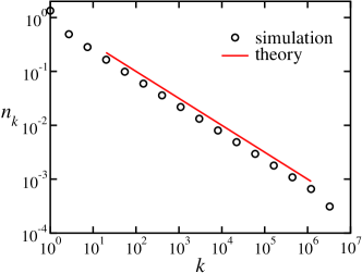
Figure 2: The normalized size distribution $n_{k}=M^{-1/2}N_{k}$ versus $k$, obtained from $10^{3}$ independent Monte Carlo realization for a total population of size $10^{7}$. The rates are $\alpha=\beta$ and $\gamma=0$. Also shown for comparison is the theoretical prediction $n_{k}\sim k^{-1/2}$.

To test the theoretical predictions, we performed Monte Carlo simulations. We focus on the no-death case ($\gamma=0$) because it can be simulated efficiently, thereby allowing us to generate populations of size up to $10^{7}$. The simulation is straightforward: an organism is picked at random. Then, with probability $\alpha/(\alpha+\beta)$ an identical organism is created (replication), while with probability $\beta/(\alpha+\beta)$, a new species is created (mutation). The simulation results are in excellent agreement with the theoretical results. For example, for the case $\alpha=\beta$, the exponent agrees with the theoretical prediction $\mu=1/2$ to within $0.1\%$. We also simulated the case where the death rate is finite and the agreement between the simulations and the theoretical predictions concerning the exponent $\mu$ was equally strong. We conclude that the numerical simulations indicate that even though the rate equations (6) and (8) are approximate, they yield asymptotically exact results for the large-rank behavior. In particular, the predicted exponent $\mu$ appears to be exact.

We also noticed that in a single realization, $N_{k}$ deviates significantly from the theoretical prediction, indicating that there are strong sample-to-sample fluctuations. This is not surprising because the populations are growing exponentially. To extract meaningful results from a single realization, it is necessary to study statistics of the variable $z=\ln k$. Using this exponentially-distributed variable, the large fluctuations are suppressed, and the power-law behavior (10) is clear.

A closely-related quantity is the total descendant population of a species, that is, the total population of all species that emanated from a given species. For example, in figure 1, the total descendant population of the first species is 7 and that of the second species is 3. Fixing the $k^{\rm th}$ species as a common ancestor, we denote by $P_{k}$ the average size of its descendant population. This quantity satisfies the initial condition $P_{k}(0)=\delta_{k,1}$ and it evolves according to

$$\frac{dP_{k}}{dt}=(\alpha+\beta-\gamma)\,P_{k}+\beta Mf_{k-1}\,.$$ (12)

Since a descendant of a descendant is also a descendant, the growth rate now accounts for mutation too, in contrast with Eq. (8). The transformation $P_{k}=M\,p_{k}$ recasts Eq. (12) into $dp_{k}/dt=\beta f_{k-1}$. Since every species is the descendant of the grand ancestor, $p_{k}=1$. Otherwise, for $k\geq 2$ one has

$$p_{k}(t)=\beta\,\int_{0}^{t}d\tau\,f_{k-1}(\tau).$$ (13)

The quantity $p_{k}$ is of course the probability that a randomly selected organism is a descendant of the $k^{\rm th}$ species. Repeating the asymptotic analysis that has been applied to Eq. (8), we find that $p_{k}(t)$ reaches an asymptotic value, $p_{k}(t)\to p_{k}(\infty)$ as $t\to\infty$, with

$$p_{k}(\infty)=\frac{1}{(k-2)!}\int_{0}^{\infty}dx\,\left[1+\frac{x}{1-\mu}\right]^{-1}x^{k-2}e^{-x}\,.$$

In the large-rank limit we have $p_{k}\sim k^{-1}$, and therefore

$$P_{k}\sim M\,k^{-1}$$ (14)

(Fig. 3). Thus, the descendant size distribution obeys a universal law as the characteristic exponent is independent of the various rates.

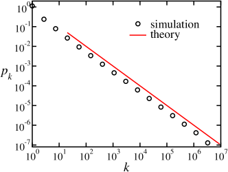
Figure 3: The descendant size distribution. Plotted is $p_{k}=M^{-1}P_{k}$ versus $k$, obtained from $10^{3}$ independent Monte Carlo realization for a population of size $M=10^{7}$. The death rate is zero ($\gamma=0$), while replication and mutation rates are equal ($\alpha=\beta$). Also shown for comparison is the theoretical prediction $p_{k}\sim k^{-1}$.

In summary, we obtained scaling laws that characterize how the population of a species and its descendant population depend on the rank. The average population of a species decays algebraically with the rank $k$, $N_{k}\sim k^{-\mu}$, with the characteristic exponent $\mu$ dependent on the rates of replication, mutation, and death. The average descendant population of a species decays in a universal fashion with the rank $k$, $P_{k}\sim k^{-1}$. Our main conclusion is that the chronological order of origination, or the rank, provides a useful characterization of biological evolution processes.

Several aspects of this model should be investigated further. Obtaining the exact behavior by properly accounting for the coupling between the total population size and the total number of species is a challenging problem. We focused on the average behavior, but statistical fluctuations must exhibit interesting behavior because the population is exponentially-growing.

Power-law distributions with different rate-dependent exponents were found for another quantity, the family size distribution, for the very same replication-mutation-death processes ds ; rh ; hv ; kwk ; jlg . In general, the various rates can not be measured directly. Since the characteristic exponents yield a constraint for the rates, such scaling-laws are useful since they reduce the number of unknown parameters in the problem.

- (1) C. Tudge, The Variety of Life (Oxford University Press, Oxford, 2000).
- (2) S. Tavaré, C. R. Marshall, O. Will, C. Soligo, and R. D. Martin, Nature 416, 726–729 (2002).
- (3) S. J. Gould, The structure of evolutionary theory (Harvard University Press, Cambridge, 2002).
- (4) J. John Sepkoski, A compendium of fossil marine animal families (Paleontological Research Institution, Ithaca, 2002).
- (5) M. S. Waterman, Introduction to computational biology: Maps, sequences and genomes (Chapman & Hall, London, 1995).
- (6) R. Durbin, S. Eddy, A. Krogh, and G. Mitchison, Biological sequence analysis (Cambridge University Press, Cambridge, 1998).
- (7) Tree of Life web project, http://www.tolweb.org/.
- (8) R. D. M. Page and E. C. Holmes, Molecular Evolution: A Phylogenetic Approach (Blackwell, Oxford, 1998).
- (9) J. Felsenstein, Inferring Phylogenies (Sinhauer, Sunderland, 2003).
- (10) G. U. Yule, Philos. Trans. Roy. Soc. London B 213, 21 (1924).
- (11) H. A. Simon, Biometrika 42, 425 (1955).
- (12) T. E. Harris, The theory of branching processes (Dover, New York, 1989).
- (13) W. J. Ewens, Mathematical population genetics (Springer, New York, 1979).
- (14) S. Altschul, R. Carroll, and D. Lipman, J. Mol. Biol. 207, 647 (1989).
- (15) W. Li, Phys. Rev. A 43, 5240 (1991).
- (16) B. G. Giraud, A. S. Lapedes, and L. C. Liu, Phys. Rev. E 58, 6312 (1998).
- (17) E. Ben-Naim and A. S. Lapedes, Phys. Rev. E 59, 7000 (1999).
- (18) W. J. Reed and B. D. Hughes, Phys. Rev. E 66, 067103 (2002).
- (19) M. A. Huynen and E. van Nimwegen, Mol. Biol. Evol. 15, 583 (1998).
- (20) E. V. Koonin, Y. Wold, and G. Karev, Nature 420, 218 (2002).
- (21) Q. Jian, N. Luscombe, and M. Gerstein, J. Mol. Biol. 313, 673 (2001).
- (22) R. Durrett and J. Schweisenberg, math.PR/0406216.
- (23) P. W. Messer, P. F. Arndt, and M. Lässig, Phys. Rev. Lett. 94, 1318103 (2005).
- (24) B. Snel, M. A. Huynen, and B. E. Dutilh, Annu. Rev. Microbiol. 59, 191 (2005).
- (25) D. E. Knuth, The Art of Computer Programming, vol. 3, Sorting and Searching (Addison-Wesley, Reading, 1998).
- (26) R. E. Horton, Bull. Geol. Soc. Amer. 56, 275 (1945).
- (27) An exact description must involve the joint population size-mutation number probability distribution.
- (28) E. Ben-Naim and P. L. Krapivsky, unpublished.