Self-optimization, community stability, and fluctuations in two individual-based models of biological coevolution

Abstract

We compare and contrast the long-time dynamical properties of two individual-based models of biological coevolution. Selection occurs via multispecies, stochastic population dynamics with reproduction probabilities that depend nonlinearly on the population densities of all species resident in the community. New species are introduced through mutation. Both models are amenable to exact linear stability analysis, and we compare the analytic results with large-scale kinetic Monte Carlo simulations, obtaining the population size as a function of an average interspecies interaction strength. Over time, the models self-optimize through mutation and selection to approximately maximize a community fitness function, subject only to constraints internal to the particular model. If the interspecies interactions are randomly distributed on an interval including positive values, the system evolves toward self-sustaining, mutualistic communities. In contrast, for the predator-prey case the matrix of interactions is antisymmetric, and a nonzero population size must be sustained by an external resource. Time series of the diversity and population size for both models show approximate $1/f$ noise and power-law distributions for the lifetimes of communities and species. For the mutualistic model, these two lifetime distributions have the same exponent, while their exponents are different for the predator-prey model. The difference is probably due to greater resilience toward mass extinctions in the food-web like communities produced by the predator-prey model.

I Introduction

Traditionally, problems in ecology and evolution have been addressed at very different levels of resolution. Typically, ecological problems are studied on a timescale of generations and often at the level of individual organisms, while issues in evolution are considered on much longer, often geological, timescales and usually at the level of species or higher-level taxa. However, in recent years it has been recognized that processes at the ecological and evolutionary scales can be strongly linked DROS01B ; THOM98 ; THOM99 ; YOSH03 . Several models have therefore been proposed, which aim to model the complex problem of coevolution in a fitness landscape that changes with the composition of the community, while spanning the disparate scales of both temporal and taxonomic resolution. Early steps in this direction were simulations of parapatric and sympatric speciation CROS70 and the coupled $NK$ model with population dynamics KAUF93 ; KAUF91 . More recent contributions include the Webworld model CALD98 ; DROS01B ; DROS04 , the Tangled-nature model CHRI02 ; COLL03 ; HALL02 and simplified versions of the latter RIKV03 ; SEVI06 ; ZIA04 , as well as network models CHOW05 ; CHOW03A . Recently, large individual-based simulations have also been performed of parapatric and sympatric speciation GAVR98 ; GAVR00 and of adaptive radiation GAVR05 . Many of these models are deliberately quite simple, aiming to elucidate universal features that are largely independent of the finer details of the ecological interactions and the evolutionary mechanisms. Such universal features may include lifetime distributions for species and communities, as well as other aspects of extinction statistics, statistical properties of fluctuations in diversity and population sizes, and the structure and dynamics of food webs that develop and change with time. By changing specific features of such simplified models, one hopes to learn which aspects influence the observed properties of the resulting communities and their development with time.

In this paper we compare and contrast two stochastic coevolution models that combine features from some of those mentioned above. In each, selection is provided by an individual-based population dynamics, while new species are provided by a low rate of mutation. The models are studied both analytically by linear stability theory, and numerically by large-scale kinetic Monte Carlo simulations. The first model (Model A) allows direct mutualistic interspecies interactions, and some of its properties were discussed previously RIKV03 ; SEVI06 ; ZIA04 . It is a simplified version of the Tangled-nature model of Jensen and coworkers CHRI02 ; COLL03 ; HALL02 . The second model (Model B) is a predator-prey model. For both models we obtain exactly the fixed-point mean population sizes and stability properties for any given community of species in the limit of vanishing mutation rate, using linear stability theory. These results enable us to define a community fitness function, cubic in the mean total population size, that is maximized at the fixed point for a given community of species. The fact that this much information can be obtained analytically makes these models uniquely well suited as benchmarks for more elaborate, but less tractable, nonlinear models.

The analytical results are followed by numerical simulations of the dynamics of both models for nonzero mutation rates. We focus on very long simulations in a regime where both diversity and population size are statistically stationary, albeit with very large, strongly correlated fluctuations and an intermittently vigorous turnover of species. We thus study the intrinsic dynamics of extinction and origination of species and communities in the absence of external perturbations. Understanding of these intrinsic fluctuations in the stationary state should enable one to estimate the community’s response to external perturbations SATO03 in a way analogous to the fluctuation-dissipation relations of statistical mechanics PATH96 .

Three main conclusions emerge from this combined analytical and numerical investigation.

• Mutations enable the models to evolve communities that tend to maximize the community fitness function, subject only to constraints that are internal to the specific model. Although there is vigorous turnover of species and communities, all communities that persist for a significant time remain in the vicinity of this maximum.

• The simulated systems exhibit power-law distributions in the lifetimes of individual species, as well as of communities, and the fluctuations in diversity and population size are characterized by approximate $1/f$ noise.

• The two models show distinct differences in the community turnover, which are reflected in differences between the power-law exponent of the community-lifetime distribution. In Model A, extinctions of species tend to be highly synchronized, such that a whole community collapses in a mass extinction on a relatively short time scale. In Model B, on the other hand, extinctions are more often limited to a subset of the resident species. This can be explained by differences between the structures of the interaction networks characterizing long-lived communities in the two models. For Model B, this network amounts to a simple food web.

The rest of this paper is organized as follows. The models are introduced in Sec. II. In Sec. III we perform a full analytical linear stability analysis, and the results are compared with large-scale kinetic Monte Carlo simulations. The simulations are described in further detail in Sec. IV, where lifetime distributions and power spectral densities also are reported. A concluding summary is presented in Sec. V. Some technical details of the derivation of the community fitness function are given in Appendix A, an analytical result for the optimum population size of Model A is obtained in Appendix B, and a discussion of the consequences of changes in several of the model parameters is found in Appendix C.

II The Models

In both models, selection is provided by the reproduction rates in an individual-based, simplified, stochastic population-dynamics model with nonoverlapping generations. This interacting birth-death process is augmented to enable evolution of new species by a mutation mechanism. The mutations act on a haploid, binary “genome” of length $L$, as introduced in Eigen’s model for molecular evolution EIGE71 ; EIGE88 . This bit string defines the species, which are identified by the integer label $I\in[0,2^{L}-1]$. Typically, only a few of these $2^{L}$ potential species are resident in the community at any one time.

Individual organisms of species $I$ reproduce asexually at the end of each generation, each giving rise to $F$ offspring individuals with probability $P_{I}$ before dying. With probability $(1-P_{I})$, they die without offspring. No individual thus survives beyond one generation. (For simplicity, the fecundity $F$ is assumed fixed, independent of both species and individual.)

During reproduction, each gene in an offspring individual’s genome may undergo mutation ($0\rightarrow 1$ or $1\rightarrow 0$) with a small probability, $\mu/L$. The mutation thus corresponds to diffusional moves from corner to corner along the edges of an $L$-dimensional hypercube GAVR99 ; GAVR04 . A mutated individual is assumed to belong to a different species than its parent, with different properties. Genotype and phenotype are thus in one-to-one correspondence in these models. This is clearly a highly idealized picture, and it is introduced to maximize the pool of different species available within the computational resources. The approximation is justified by a large-scale computational study of a version of Model A, in which species that differ by as many as $L/2$ bits have correlated properties SEVI06 . Quite remarkably, this study reveals that the correlated model has long-time dynamical properties very similar to the uncorrelated Model A studied here.

The reproduction probability $P_{I}(t)$ for an individual of species $I$ in generation $t$ depends on the individual’s ability to utilize the amount of external resources available, $R$, and on its interactions with the population sizes $n_{J}(t)$ of all the species present in the community at that time. The dependence of $P_{I}$ on the set of $n_{J}$ is determined by an interaction matrix $\bf M$ SOLE96B with elements ${M}_{IJ}\in[-1,1]$ in a way defined specifically in the next paragraph. We emphasize that $\bf M$ is chosen randomly at the beginning of each simulation run and is subsequently kept constant throughout the run. If ${M}_{IJ}$ is positive and ${M}_{JI}$ is negative, then $I$ is a predator and $J$ its prey, and vice versa. If both matrix elements are positive, the species interact directly in a mutualistic way, while both elements negative implies direct competition.

Specifically, the reproduction probability for species $I$, $P_{I}(t)$, depends on $R$ and the set $\{n_{J}(t)\}$ through the nonlinear form,

$$P_{I}(t)=\frac{1}{1+\exp[-\Delta_{I}(R,\{n_{J}(t)\})]}\;,$$ (1)

with the density dependent argument

$$\Delta_{I}(R,\{n_{J}(t)\})=-b_{I}+\eta_{I}R/N_{\rm tot}(t)+\sum_{J}M_{IJ}n_{J}(t)/N_{\rm tot}(t)-N_{\rm tot}(t)/N_{0}\;.$$ (2)

Here $b_{I}$ can be seen as the “cost” of reproduction (always positive), and $\eta_{I}$ (positive for primary producers or autotrophs, and zero for consumers or heterotrophs) is the ability of individuals of species $I$ to utilize the external resource $R$. The latter is renewed at the same level each generation. It does not have independent dynamics. The total population size is $N_{\rm tot}(t)=\sum_{J}n_{J}(t)$, and the constant $N_{0}$ is an environmental carrying capacity MURR89 ; VERH1838 that prevents $N_{\rm tot}(t)$ from diverging to infinity. It may be seen as representing implicit resource limitations not explicitly included in $R$, such as available space.

For large positive $\Delta_{I}$, the individual almost certainly reproduces, giving rise to $F$ offspring, while for large negative $\Delta_{I}$, it almost certainly dies without offspring. The reproduction probability $P_{I}$, together with its argument $\Delta_{I}$, play the role of a functional response for this class of models DROS01B ; KREB01 . The two externally determined parameters that influence the population size, the resource term $R$ and the carrying capacity $N_{0}$, play very different roles. From Eq. (2) it is seen that $R$ encourages population growth, especially for small total population sizes, while it has very little effect for large $N_{\rm tot}$. It can thus be thought of as representing a finite amount of available food. The carrying capacity $N_{0}$, on the other hand, always discourages growth, but its effect is only appreciable for large population sizes. It cannot maintain a nonzero population by itself and is thus best thought of as representing an overall limitation, such as finite available space. If $R=0$, a nonzero population can therefore only be maintained by mutually positive interspecies interactions. This rather unrealistic aspect is shared by the Tangled-nature model CHRI02 ; COLL03 ; HALL02 .

In this work, the model parameters are chosen to represent the realistic situation that the number of species resident in the community at any time is much smaller than the number of potential species (i.e., that $\mathcal{N}(t)\ll 2^{L}$), and also that $\mathcal{N}(t)\ll N_{\rm tot}(t)$.

An analytic approximation describing the time development of the mean population sizes (averaged over independent realizations), $\langle n_{I}(t)\rangle$, can be written as a set of coupled difference equations,

$$\langle n_{I}(t+1)\rangle = \langle n_{I}(t)\rangle FP_{I}(R,\{\langle n_{J}(t)\rangle\})[1-\mu]$$ (3)

$$+(\mu/L)F\sum_{K(I)}\langle n_{K(I)}(t)\rangle P_{K(I)}(R,\{\langle n_{J}(t)\rangle\})+O(\mu^{2})\;,$$

where $K(I)$ is the set of species that can be generated from species $I$ by a single mutation (“nearest neighbors” of $I$ in genotype space).

II.1 Model A

Model A was introduced and studied in RIKV03 ; ZIA04 . In this model, the $M_{IJ}$ for $I\neq J$ are stochastically independent and uniformly distributed on $[-1,+1]$, while the intra-species interactions $M_{II}=0$. The external resource $R$ and the reproduction costs $b_{I}$ are equal to zero, and the total population size $N_{\rm tot}(t)$ is limited only by the carrying capacity $N_{0}$. The model is found to evolve through a succession of quasi-stable, mutualistic communities.

II.2 Model B

Model B is a predator-prey model. This is implemented by making the off-diagonal part of $\bf M$ antisymmetric. In order to keep the connectance of the resulting communities consistent with food webs observed in nature DUNN02 ; GARL04 , the $(M_{IJ},M_{JI})$ pairs are chosen nonzero with probability $c=0.1$. The nonzero elements in the upper triangle of $\bf M$ are chosen independently and uniformly on $[-1,+1]$. This model does not include a population-limiting carrying capacity [i.e., formally, $N_{0}=\infty$ in Eq. (2)], and the community is supported by a constant external resource, $R$. Only a proportion $p$ of the $2^{L}$ potential species are producers that can directly utilize the resource (for the numerical data reported here, we use $p=0.05$). Thus, with probability $(1-p)$ the resource coupling $\eta_{I}=0$, representing consumers, while with probability $p$ the $\eta_{I}$ are independently and uniformly distributed on $(0,+1]$, representing producers of varying efficiency. In addition to these constraints on $\bf M$, we require that producers ($\eta_{I}>0$) always are the prey of consumers ($\eta_{I}=0$). In other words: the case $\eta_{I}>0$ and $\eta_{J}=0$ with $M_{IJ}\equiv-M_{JI}>0$ is forbidden. Whenever it occurs, this situation is corrected during the construction of $\bf M$ by reversing the signs of $M_{IJ}$ and $M_{JI}$ for the pair in question. Consumers at higher trophic levels are allowed, and they are indeed observed in the resulting communities (see further discussion in Sec. IV). The population sizes are limited by independent reproduction costs $b_{I}$ that are uniformly distributed on $(0,+1]$, and by negative intra-species interactions $M_{II}$ independently and uniformly distributed on $[-1,0)$. The model is found to evolve through a succession of quasi-stable, food-web like communities. Some preliminary numerical results were presented in RIKV05A .

III Linear Stability Analysis

The form of $\Delta_{I}$ in Eq. (2) represents frequency-dependent interactions that describe universal competition and absence of adaptive foraging, and so is not very realistic. However, the normalization by $N_{\rm tot}(t)$ has the advantage that it turns Eq. (3) with $\mu=0$ into a set of linear equations for the average population sizes in the fixed-point community corresponding to a particular set of species. The set of equations can be solved analytically to give the average total population size, as well as the average population size of each species and the stability properties of the community. This mean-field level analysis also enables us to construct a community fitness function that for a given set of species is maximized by the fixed-point community, and whose width is proportional to the size of the population fluctuations around the fixed point, caused by the statistical birth-death process. (For a detailed discussion of the fluctuations in Model A in the absence of mutations, see ZIA04 .) For small mutation rates, this picture remains valid as a description of the population fluctuations on relatively short time scales, where the species composition of the community remains constant, except for small populations of unsuccessful mutants.

III.1 Fixed-point communities

To obtain the stationary solution of Eq. (3) with $\mu=0$ for a community of $\mathcal{N}$ species, we require $P_{I}=1/F$ for all $\mathcal{N}$ species. Equations (1) and (2) then yield the $\mathcal{N}$ linear relations

$$-\tilde{b}_{I}+\eta_{I}\frac{R}{N_{\rm tot}^{*}}+\sum_{J}M_{IJ}\frac{n_{J}^{*}}{N_{\rm tot}^{*}}-\frac{N_{\rm tot}^{*}}{N_{0}}=0\;,$$ (4)

where $\tilde{b}_{I}=b_{I}-\ln(F-1)$. (For simplicity, we have dropped the $\langle\;\rangle$ notation for the average population sizes. The asterisk superscripts denote fixed-point solutions.) In a vector notation where $\vec{v}$ is a column vector and $\vec{v}^{T}$ its conjugate row vector, $\vec{n}^{*}$ is the column vector composed of the $\mathcal{N}$ nonzero $n_{I}^{*}$, while $\vec{1}^{T}$ is an $\mathcal{N}$-dimensional row vector composed entirely of ones. Thus, the total population size is given by $N_{\rm tot}^{*}\equiv\sum_{I}n_{I}^{*}=\vec{1}^{T}\vec{n}^{*}$, and Eq. (4) takes the matrix form

$$-\vec{\tilde{b}}N_{\rm tot}^{*}+\vec{\eta}R+{\hat{{\bf M}}}\vec{n}^{*}-\vec{1}(N_{\rm tot}^{*})^{2}/N_{0}=0\;.$$ (5)

Here, $\vec{\tilde{b}}$ is the column vector whose elements are $\tilde{b}_{I}$, $\vec{\eta}$ is the column vector whose elements are $\eta_{I}$ (in both cases including only those $\mathcal{N}$ species that have nonzero $n_{I}^{*}$), $\hat{\bf M}$ is the corresponding $\mathcal{N}\times\mathcal{N}$ submatrix of $\bf M$, and $\vec{1}$ is an $\mathcal{N}$-dimensional column vector of ones. The solution for $\vec{n}^{*}$ is

$$\vec{n}^{*}=-{\hat{\bf M}}^{-1}\left[\vec{\eta}R-\vec{\tilde{b}}N_{\rm tot}^{*}-\vec{1}(N_{\rm tot}^{*})^{2}/N_{0}\right]\;,$$ (6)

where ${\hat{\bf M}}^{-1}$ is the inverse of ${\hat{\bf M}}$. (See below for a discussion of the effects of a singular $\hat{\bf M}$.) To find each $n_{I}^{*}$, we must first obtain $N_{\rm tot}^{*}\equiv\vec{1}^{T}\vec{n}^{*}$. Multiplying Eq. (6) from the left by $\vec{1}^{T}$, we obtain the quadratic equation for $N_{\rm tot}$,

$$R\mathcal{E}+\Theta N_{\rm tot}^{*}-(N_{\rm tot}^{*})^{2}/N_{0}=0\;.$$ (7)

The coefficients,

$$\Theta=\frac{1-\vec{1}^{T}{\hat{\bf M}}^{-1}\vec{\tilde{b}}}{\vec{1}^{T}{\hat{\bf M}}^{-1}\vec{1}} \mathcal{E}=\frac{\vec{1}^{T}{\hat{\bf M}}^{-1}\vec{\eta}}{\vec{1}^{T}{\hat{\bf M}}^{-1}\vec{1}}\;,$$ and (8)

can be viewed as an effective interaction strength and an effective coupling to the external resource, respectively. Approximate expressions for $\Theta$ and $\mathcal{E}$ that are less accurate but more intuitive are obtained in Appendix A. The nonnegative solution of Eq. (7) is

$$N_{\rm tot}^{*}=\frac{\Theta N_{0}}{2}+\sqrt{\left(\frac{\Theta N_{0}}{2}\right)^{2}+R\mathcal{E}N_{0}}\;.$$ (9)

Figure 1(a) shows $N_{\rm tot}^{*}$ as a function of $\Theta$ for two choices of $N_{0}$ and $R$ at fixed $\mathcal{E}$. Special cases of the solution are

$$N_{\rm tot}^{*}=\left\{\begin{array}[]{lllll}\Theta{N_{0}}&\mbox{for}&R=0&\mbox{and}&\Theta\geq 0\\ 0&\mbox{for}&R=0&\mbox{and}&\Theta\leq 0\\ \sqrt{R\mathcal{E}N_{0}}&\mbox{for}&\Theta=0&\mbox{and}&\mathcal{E}\geq 0\\ -R\mathcal{E}/\Theta&\mbox{for}&N_{0}=\infty&\mbox{and/or}&\vec{1}^{T}\hat{\bf M}^{-1}\vec{1}=0\end{array}\right.\;.$$

To find each $n_{I}^{*}$ separately, we now only need to insert $N_{\rm tot}^{*}$ in Eq. (6).

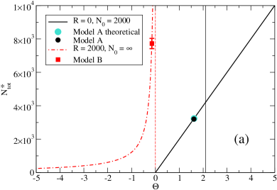
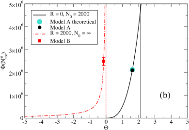
Figure 1: (Color online.) Solutions for (a) the total fixed-point population size $N_{\rm tot}^{*}$ and (b) the maximum community fitness function $\Phi_{\rm max}=\Phi(N_{\rm tot}^{*})$. Both are shown vs $\Theta$ for fixed $\mathcal{E}=0.61$. The solid vertical lines represent the absolute maximum value for $\Theta$ in Model A, while the dotted vertical lines represent the analogous limit for Model B. The points marked “Model A” and “Model B” were obtained from large-scale Monte Carlo simulations as described in the text. The calculation of the point marked “Model A theoretical” is described in Appendix B.

Only those $\vec{n}^{*}$ that have all positive elements can represent a feasible community ROBE74 . If ${\hat{\bf M}}={\bf 0}$ or is otherwise singular, the set of equations (5) is inconsistent for $\mathcal{N}>1$, unless $\tilde{b}_{I}$ and $\eta_{I}$ both are independent of $I$. The only possible stationary community then consists of one single species, the one with the largest value of $-\tilde{b}_{I}$ for Model A or the one with the largest $\eta_{I}/\tilde{b}_{I}$ for Model B. This is a trivial example of competitive exclusion ARMS80 ; DENB86 ; HARD60 , and stable multispecies coexistence in these models requires a nonsingular interaction matrix .

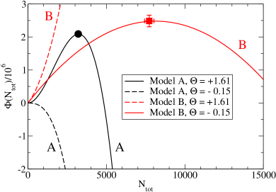
Figure 2: (Color online.) The community fitness function $\Phi$, shown vs $N_{\rm tot}$ for Model A (black) and Model B (gray, red online). For Model A the parameters are: $F=4$, $R=0$, and $N_{0}=2000$. For Model B they are: $F=2$, $R=2000$, $\mathcal{E}=0.61$, and $N_{0}=\infty$. The values of $\Theta$ used are $1.61$, corresponding to the average value taken by Model A in the simulations, and $-0.15$, corresponding to the average value taken by Model B. $\Phi(N_{\rm tot})$ has a nontrivial maximum for Model A at positive $\Theta$ (solid black curve marked A), and for Model B at negative $\Theta$ (solid gray curve marked B (red online)). The circular and square data points are the results of Monte Carlo simulations and correspond to the equally shaped points in Fig. 1. They lie very close to the maximum of $\Phi(N_{\rm tot})$ for each model. The dashed curves show the physically inaccessible cases of Model A with $\Theta<0$ (stable, absorbing state at $N_{\rm tot}=0$) and Model B with $\Theta>0$ (monotonically increasing $\Phi(N_{\rm tot})$).

Equation (7) can be seen as a maximization condition for a community fitness function,

$$\Phi(N_{\rm tot})=\left(1-\frac{1}{F}\right)\left(R\mathcal{E}N_{\rm tot}+\frac{\Theta}{2}N_{\rm tot}^{2}-\frac{1}{3N_{0}}N_{\rm tot}^{3}\right)\;,$$ (10)

which is cubic in $N_{\rm tot}$ . The dependence of $\Phi$ on $N_{\rm tot}$ is shown in Fig. 2 for Models A and B at two different values of $\Theta$. In each model, the maximum of $\Phi$ represents the fixed-point value of $N_{\rm tot}$, while its width gives a measure of the extent of the fluctuations about the fixed-point population in a community of fixed composition ZIA04 . The maximum value of $\Phi$ with respect to $N_{\rm tot}$, $\Phi_{\rm max}=\Phi(N_{\rm tot}^{*})$, is shown in Fig. 1(b) vs $\Theta$ for two different values of $N_{0}$ at fixed $\mathcal{E}$.

From Eq. (III.1) and Fig. 1(a) it is seen that Model A (finite $N_{0}$ and $R=0$) undergoes a transcritical bifurcation or exchange of stabilities CRAW91 ; STRO94 at $\Theta=0$. For $\Theta\leq 0$, $N_{\rm tot}$ vanishes, while for $\Theta>0$ it increases linearly with $\Theta$ . Such behavior as a function of a control parameter is common in many nonequilibrium systems. In addition to population dynamics and the logistic map (to which the present models with $\mu=0$ are closely related), these also include lasers and autocatalytic chemical reactions HAKE77 ; STRO94 . On the other hand, for Model B ($N_{0}=\infty$ and $R>0$), $N_{\rm tot}$ diverges to infinity as $\Theta$ approaches zero from below, and it would be infinite for $\Theta\geq 0$.

The results discussed in the previous paragraphs would not be of evolutionary relevance if $\Theta$ were just an externally fixed control parameter, as it would be in the absence of extinctions and mutations. However, mutations enable the community not only to maximize $\Phi(N_{\rm tot})$ for fixed parameters, but also to change the parameters in response to new mutations, leading to the possibility of further increasing $\Phi_{\rm max}$. Numerical results from the large-scale kinetic Monte Carlo simulations discussed in Sec. IV show that, on average, the communities initially progress toward, and later settle down to fluctuate near, the maximum value of $\Theta$ (and thus the maximum value of $\Phi_{\rm max}$) compatible with the constraints on $\bf M$ and $\tilde{\vec{b}}$. These constraints depend on the specific model as follows. For Model A, which allows direct mutualistic interactions (i.e., $M_{IJ}$ and $M_{JI}$ both positive), $\Theta$ can be positive, thus enabling communities with nonzero population size, even for $R=0$. For the predator-prey Model B, on the other hand, the antisymmetric structure of $\bf M$ forces $\Theta$ to be nonpositive. A detailed discussion of the time evolution of the mean-field parameters, $\Theta$, $\mathcal{E}$, $N_{\rm tot}^{*}$, and $\Phi_{\rm max}$, is given for both models in Sec. IV.1.

In Monte Carlo simulations of Model A (in which the off-diagonal elements of $\bf M$ are uncorrelated and uniformly distributed on $[-1,+1]$), it was found that, after the initial period characterized by an average positive trend in the mean-field parameters, the community spent most of its time in a succession of quasi-steady states (QSSs), separated by brief bursts of intense evolutionary activity RIKV03 . All the QSSs studied in detail were found to be mutualistic, with $\overline{M_{IJ}}=0.78\pm 0.03$. [Here, the overbar represents averages over all the ten QSSs listed in Table I of RIKV03 .] The average of $N_{\rm tot}$, taken over all the 16 realizations of $2^{25}$ generations that were studied, was ${\overline{N_{\rm tot}}}=3201\pm 8$. (The average over only the ten QSSs agrees with the total average to within the statistical errors, showing that the periods when the system is not in a QSS contribute negligibly to the overall time averages.) From these averages we can use Eqs. (III.1) and (10) to estimate the average mean-field quantities, $\overline{\Theta}=1.61\pm 0.01$ and $\overline{\Phi_{\rm max}}=(2.09\pm 0.06)\times 10^{6}$. In Fig. 1(a), ${\overline{N_{\rm tot}}}$ is shown vs $\overline{\Theta}$ as a black dot, while the corresponding value of $\overline{\Phi_{\rm max}}$ is shown the same way in Fig. 1(b).

The results for Model B that are included in Fig. 1 were also obtained from Monte Carlo simulations of 2²⁵ generations. (See Sec. IV for further details.) The parameter values used in the figure were extracted as the average values from thirteen QSS communities identified at late times in twelve independent simulation runs: $\overline{\mathcal{E}}=0.61\pm 0.04$ and $\overline{\Theta}=-0.15\pm 0.01$. The value of the total population size given in the figure is the total time average over the simulations, averaged over all twelve runs, ${\overline{N_{\rm tot}}}=7726\pm 303$. (Like for Model A, averages over only the particular observed QSS communities agree with this total average to within the error bars.) The large uncertainty in ${\overline{N_{\rm tot}}}$ is a direct consequence of the steep slope of $N_{\rm tot}^{*}$ versus $\Theta$ closely below $\Theta=0$ for Model B (see Fig. 1(a)). From these estimates and Eq. (10) we further get the estimate $\overline{\Phi_{\rm max}}=(2.49\pm 0.18)\times 10^{6}$.

III.2 Stability of fixed-point communities

The internal stability of an $\mathcal{N}$-species fixed-point community is obtained from the matrix of partial derivatives,

$$\left.\frac{\partial n_{I}(t+1)}{\partial n_{J}(t)}\right|_{\vec{n}^{*}}=\delta_{IJ}+\Lambda_{IJ}\;,$$ (11)

where $\delta_{IJ}$ is the Kronecker delta and $\Lambda_{IJ}$ are elements of the community matrix $\bf\Lambda$ MURR89 . Straightforward differentiation yields

$$\Lambda_{IJ}=\left(1-\frac{1}{F}\right)\frac{n_{I}^{*}}{N_{\rm tot}^{*}}\left[M_{IJ}-\frac{R\eta_{I}+({\hat{\bf M}}\vec{n}^{*})_{I}}{N_{\rm tot}^{*}}-\frac{1}{N_{0}}\right]\;,$$ (12)

where $({\hat{\bf M}}\vec{n}^{*})_{I}$ is the element of ${\hat{\bf M}}\vec{n}^{*}$ corresponding to species $I$. In order for deviations from the fixed point to decay monotonically in magnitude, the magnitudes of the eigenvalues of the matrix of partial derivatives in Eq. (11), ${\bf\Lambda}+{\bf 1}$ where $\bf 1$ is the $\mathcal{N}$-dimensional unit matrix, must be less than unity. The values of the fecundity $F$ that are used in this work (4 for Model A and 2 for Model B) were chosen to satisfy this requirement for $\mathcal{N}=1$.

Since new species are created by mutations, we must also study the stability of the fixed-point community toward “invaders.” Consider a mutant invader $i$. Then its multiplication rate, in the limit that $n_{i}\ll n_{J}$ for all $\mathcal{N}$ species $J$ in the resident community, is given by

$$\frac{n_{i}(t+1)}{n_{i}(t)}=\frac{F}{1+\exp\left[-\Delta_{i}(R,\{n_{J}^{*}\})\right]}\;.$$ (13)

The Lyapunov exponent, $\ln[n_{i}(t+1)/n_{i}(t)]$, is the invasion fitness of the mutant with respect to the resident community DOEB00 ; METZ92 . A characteristic feature of the QSS communities observed in both Model A and Model B is that only about 1% of the mutants that are separated from the resident community by a single mutation (“nearest-neighbor species”) have multiplication rates above unity (and most of those are between 1.0 and 1.1). In fact, this is true only to a slightly lesser degree for mutants separated by two or three mutations from the resident species (“next-nearest neighbors” and “third-nearest neighbors”) RIKV03 . Thus, a string of rather unsuccessful, or at best neutral, mutations is necessary to bring significant change to a QSS community – a fact that to a large extent accounts for their high degree of stability.

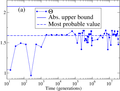
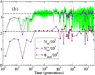
Figure 3: (Color online.) Typical time series of the mean-field, fixed-point parameters for Model A ($N_{0}=2000$, $R=0$, $F=4$, $L=13$, and $\mu=10^{-3}$), emphasizing the transient early-time regime by using a logarithmic time axis. (a) The effective interaction strength $\Theta$. The solid, horizontal line is the absolute upper bound on $\Theta$ for Model A, $(1+\ln 3)\approx 2.10$, while the dashed, horizontal line is the most probable value, 1.618. Both are derived in Appendix B. (b) The fixed-point population size $N_{\rm tot}^{*}$ and the corresponding maximum value of the community fitness function, $\Phi_{\rm max}$. The dashed, horizontal lines are the corresponding values obtained from the most probable value of $\Theta$. For comparison, the simulated total population size (sampled on a much finer time scale) is shown light gray (green online) in the background.

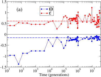
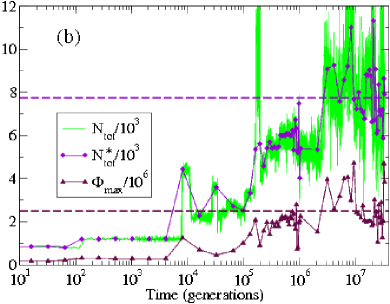
Figure 4: (Color online.) Typical time series of the mean-field, fixed-point parameters for Model B ($N_{0}=\infty$, $R=2000$, $F=2$, $L=13$, and $\mu=10^{-3}$), emphasizing the transient early-time regime by using a logarithmic time axis. (a) The effective interaction strength $\Theta$ and the effective coupling to the external resource, $\mathcal{E}$. The solid, horizontal line at zero is the absolute upper bound on $\Theta$ for Model B, while the dashed, horizontal lines are the averages over late-time communities, also shown as points in Figs. 1 and 2. (b) The fixed-point population size $N_{\rm tot}^{*}$ and the corresponding maximum value of the community fitness function, $\Phi_{\rm max}$. The dashed, horizontal lines are obtained the same way as in (a). For comparison, the simulated total population size (sampled on a much finer time scale) is shown light gray (green online) in the background.

IV Comparison of Dynamical Features

In this section we go beyond the mean-field treatment of the previous sections to compare and contrast some of the dynamical features observed in long kinetic Monte Carlo simulations of Model A and Model B. For both models we performed multiple simulations of $2^{25}=33\,554\,432$ generations . with a genome of length $L=13$ ($2^{13}=8192$ potential species) and a mutation rate per individual of $\mu=10^{-3}$. The fecundity $F$ was set to 4 for Model A and 2 for Model B.

The model parameters used in our simulations are chosen for computational feasibility with a view to keeping the system in the realistic regime where $\mathcal{N}(t)\ll 2^{L}$ and $\mathcal{N}(t)\ll N_{\rm tot}(t)$ at all times. At the same time, we want to study the dynamics during the late-time, statistically stationary regime, which should therefore be reached in a reasonable time. As a result of these restrictions, $L$, $R$, and $N_{0}$ are quite small, while $\mu$ is quite large, compared to natural populations. Results of tests for Model B with larger $L$ and $R$ and smaller $\mu$ are summarized in Appendix C. Analogous, but less exhaustive tests for Model A (not reported in detail here, but see brief summary in Appendix C) yield similar results. These tests indicate that the products $R\mu$ for Model B and $N_{0}\mu$ for Model A are proportional to the average number of mutant individuals produced per generation, $\overline{N_{\rm tot}}\mu$. We also note that this number is half of the universal biodiversity number in Hubbell’s neutral theory of biodiversity HUBB01 . Even though the species in the models studied here are strongly interacting, this parameter appears to play a similar role in determining the average diversity as it does in the neutral theory. Furthermore, the power laws that are observed and discussed in Sec. IV.2 are found to be robust, even against parameter changes that change $R\mu$.

IV.1 Evolution of mean-field parameters in the transient regime

The simulation runs were started with 100 individuals of a single species (or of a single producer species for Model B) and allowed to evolve under the dynamics described in Sec. II. At time points sampled at approximately constant intervals on a logarithmic scale, the “stable core” of the community was identified as follows. The fixed-point population sizes for the species present in the community at that time were calculated according to Eq. (6), and species corresponding to negative population sizes were excluded (starting from the one with the smallest simulated population size) until a stable, feasible community was obtained. This procedure was found to essentially correspond to removing species with populations below 100, which mostly were unsuccessful mutants of the “core” species. Once the core community was identified, the corresponding mean-field parameters $\Theta$, $\mathcal{E}$ (for Model B only), $N_{\rm tot}^{*}$, and $\Phi_{\rm max}$ were calculated from Eqs. (8) through (10).

Typical time series of these mean-field parameters are shown in Figs. 3 and 4, in which the early-time transient regime is emphasized by using a logarithmic time axis. For both models a clear tendency is seen for the mean-field parameters to increase during the transient regime, for so to fluctuate randomly about their long-time averages during the the later-time, statistically stationary regime. Both models thus evolve from an initial low-population community, toward a sequence of QSS communities that optimize their population sizes, subject to the constraints inherent in the respective models.

IV.2 Long-time dynamics in the statistically stationary regime

Here we concentrate on comparing and contrasting the dynamical properties of the two models in the statistically stationary regime that follows the transient regime discussed above. The emphasis will be on the temporal fluctuations of the total population sizes and the diversities of the resulting communities.

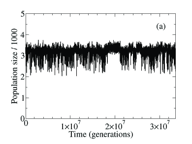
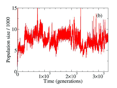
Figure 5: (Color online.) Typical time series of the total population sizes, $N_{\rm tot}(t)$, for Monte Carlo runs of $2^{25}=33\,554\,432$ generations each. To reduce the size of the figure file, the data are sampled only once every 2048 generations. While this slightly reduces the apparent range of the short-time fluctuations, the general shapes of the time series are preserved. The data are from the same runs shown in Figs. 3 and 4. (a) Model A. (b) Model B.

Typical time series of the total population sizes $N_{\rm tot}(t)$ are shown in Fig. 5. They are characterized by QSSs on different time scales, separated by periods of high evolutionary activity. In addition to the total population sizes, we also studied the diversities, defined as the number of major resident species. In order to obtain an approximation for the number of major, or “core” species (which can be thought of as the wildtypes in a quasi-species model EIGE71 ; EIGE88 ), we filter out the low-population species that are most likely unsuccessful mutants of the wildtypes. This is achieved by using the exponential Shannon-Wiener diversity index KREB89 ,

$$D(t)=e^{S[\{n_{I}(t)\}]}\;,$$ (14)

where

$$S[\{n_{I}(t)\}]=-\sum_{\{I|\rho_{I}(t)>0\}}\rho_{I}(t)\ln\rho_{I}(t)$$ (15)

with $\rho_{I}(t)=n_{I}(t)/N_{\rm tot}(t)$ is the information-theoretical entropy SHAN48 ; SHAN49 . Typical time series for $D(t)$ in the two models are shown in Fig. 6. Just like in the time series for the total population sizes, the intermittent structure consisting of QSSs on different timescales, separated by periods of high evolutionary activity, is clearly seen.

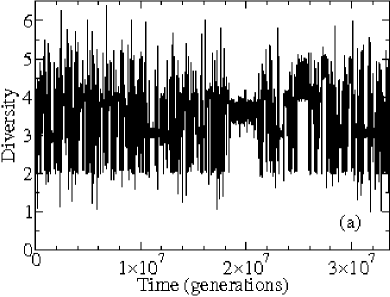
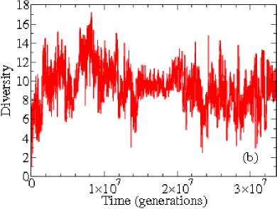
Figure 6: (Color online.) Typical time series of the exponential Shannon-Wiener diversity index $D(t)$ in the same $2^{25}$-generations Monte Carlo runs shown in Fig. 5. The data were downsampled as in Fig. 5. (a) Model A. (b) Model B.

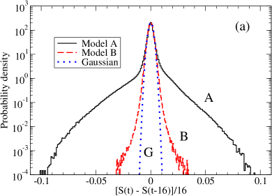
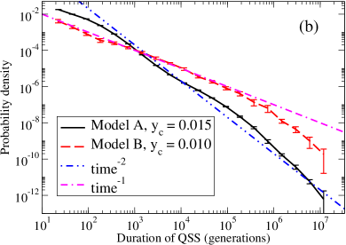
Figure 7: (Color online.) (a) Normalized histograms representing the probability density of the logarithmic derivative of the diversity, ${\rm d}S(t)/{\rm d}t$. The data were averaged over 16 generations in each run, and then averaged over 16 independent runs for Model A (solid, marked A) and 12 runs for Model B (dashed, marked B). The central parts of both histograms are well fitted by a Gaussian (dotted, marked G). (b) Log-log plot of normalized histograms representing the probability density of the durations of QSSs, estimated as the periods between times when $|{\rm d}S(t)/{\rm d}t|$ exceeds a cutoff $y_{c}$ (${\rm d}S(t)/{\rm d}t$ was averaged over 16 generations as in part (a)). Model A (solid) and Model B (dashed). Results for Model A were averaged over 16 runs, and for Model B over 12 runs. The error bars are standard errors, based on the spread between runs. The two dot-dashed straight lines represent time^-2 and time^-1 power laws, respectively.

Statistical information for characteristic time intervals that describe the dynamics can be extracted from our data. One such time interval is the duration of a QSS. One way to determine this is to use a cutoff on the magnitude of the diversity fluctuations, whose probability densities for the two models are shown in Fig. 7(a). For both models, the probability densities consist of a Gaussian central part representing the fluctuations during the QSS periods ZIA04 , flanked by “wings” that correspond to the large fluctuations during the evolutionarily active periods. We choose a cutoff $y_{c}=0.015$ for Model A and 0.010 for Model B, in both cases corresponding to the transition region between the Gaussian central peak and the wings. The duration of a single QSS then corresponds to the time interval between consecutive times when $|{\rm d}S(t)/{\rm d}t|$ exceeds $y_{c}$. Log-log plots of the resulting probability densities for the durations of QSSs in the two models are shown together in Fig. 7(b). While both show approximate power-law behavior over five decades or more in time, there is an important difference: the exponent for Model A is near $-2$, while for Model B it is closer to $-1$.

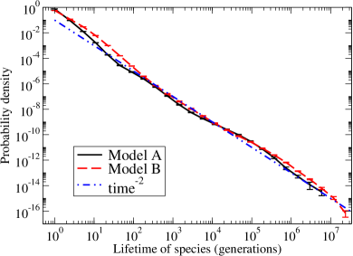
Figure 8: (Color online.) Log-log plot of normalized histograms representing the probability density of the lifetime of a particular species. Model A (solid) and Model B (dashed). Results for Model A were averaged over eight runs, and for Model B over 12 runs. The error bars were calculated as in Fig. 7(b). The dot-dashed straight line represents a time^-2 power law.

A different time interval of interest is the lifetime of a particular species, defined as the time between its origination and eventual extinction. Log-log plots of histograms of the species lifetimes in the two models are shown in Fig. 8. In contrast to the case of the QSS durations, the species-lifetime distributions are very close for the two models, both showing approximate time^-2 behavior over near seven decades in time. The observed exponent is significantly different from $-3/2$, which would correspond to the simple hypothesis that the lifetime distributions simply correspond to the first-return-time distribution for a random walk of $n_{I}$ NEWM05 ; NEWM03 . On the other hand, a lifetime distribution with an exponent of $-2$ is consistent with a stochastic branching process PIGO05 . (Simulations of neutral versions of both models also yield species lifetime distributions that decay approximately as time^-2, but with a sharp cutoff near 10⁴ generations.) Lifetime distributions for marine genera that are compatible with a power law with an exponent in the range $-1.5$ to $-2$ have been obtained from the fossil record NEWM03 ; NEWM99B . However, the possible power-law behavior in the fossil record is only observed over about one decade in time – between 10 and 100 million years – and other fitting functions, such as exponential decay, are also possible. Nevertheless, it is reasonable to conclude that the numerical results obtained from complex, interacting evolution models that extend over a large range of time scales support interpretations of the fossil lifetime evidence in terms of nontrivial power laws.

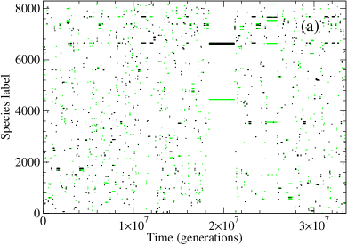
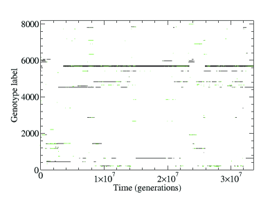
Figure 9: (Color online.) Plots showing the labels $I$ of the most highly populated species vs time. The data are for the same $2^{25}$-generation Monte Carlo runs shown in Figs. 3–6. Gray (green online): $n_{I}\in[101,1000]$. Black: $n_{I}\geq 1001$. (a) Model A. (b) Model B. For clarity, only producer species are shown for this model. The consumer species give a similar picture. See further discussion in the text.

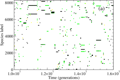
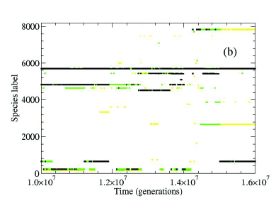
Figure 10: (Color online.) Magnified version of Fig. 9, showing times between $1.0\times 10^{7}$ and $1.6\times 10^{7}$ generations. In addition to the species shown in Fig. 9, the ones with $n_{I}\in[11,100]$ are also shown (light gray, yellow online). (a) Model A. (b) Model B. See further discussion in the text.

The difference in the power laws for the QSS durations and the species lifetimes is a puzzling result. A likely explanation can be gleaned from the data shown in Figs. 9 and 10. These show the species labels of highly populated species as functions of time for both models. From Figs. 9(a) and 10(a) it is seen that all or most of the horizontal lines representing populated species at a given time for Model A start and stop almost simultaneously, indicating that species originations and extinctions in this model are highly synchronized. In other words: whole communities in Model A tend to go extinct and be replaced with an entirely new community within a short time. In contrast, in Figs. 9(b) and 10(b) the different horizontal species lines for Model B stop and start at different times. This indicates that communities in this model are much more robust, and extinction events seldom wipe out more than a part of the total community. Thus, QSSs would be expected to be more long-lived (but also less clearly defined) for Model B, than for Model A. This theory is supported by the strikingly different QSS community structures produced by the two models, shown in Fig. 11. The typical QSS community shown for Model A is a small cluster of mutualistically interacting species, while the typical community shown for Model B has the character of a simple food web. Extinctions in the latter are likely to be confined to a single branch of the web. A detailed discussion of the community structures generated by Model B, including comparisons with data from real food webs, is found in RIKV06B .

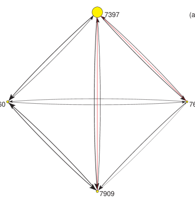
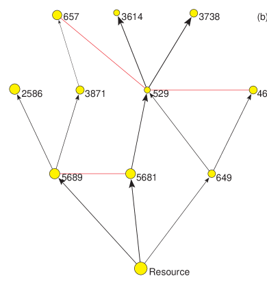
Figure 11: (Color online.) Typical QSS core communities observed in simulations of the two models. The numbers are the species labels $I$, and the sizes of the circles represent the individual species’ fixed-point populations, obtained from Eq. (6). A black arrow pointing toward species $I$ indicates a positive $M_{IJ}$, with magnitude indicated by the line thickness and size of the arrow head. The thin gray lines without arrowheads (red online) connect nearest neighbors in genotype space. (a) Model A. This particular QSS community is the one included in Table 2 of ZIA04 and line 10 of Table I of RIKV03 . (b) Model B. This is the food web representing the QSS community existing between 15 and 18 million generations in the simulation shown in Figs. 4, 5(b), 6(b), 9(b), and 10(b). It has three trophic levels above the resource node.

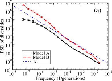
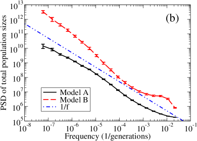
Figure 12: (Color online.) Log-log plots of PSDs of (a) the diversities $D(t)$ and (b) the total population sizes $N_{\rm tot}(t)$ for Model A and Model B. The PSDs are averaged over each octave in frequency, and then over 16 runs for Model A and 12 runs for Model B. The error bars were calculated as in Fig. 7(b). The dashed straight lines represent $1/f$ power-law behavior.

The arbitrariness inherent in the cutoff that must be used to extract QSS duration distributions from fluctuations in the diversity or other time series can to some extent be eliminated by mapping distributions obtained with different cutoffs onto a common scaling function PACZ96 ; RIKV05A . However, an analysis method that completely avoids cutoffs is that of calculating power spectral densities (the square of the temporal Fourier transform). Power spectra (PSDs) are therefore shown in Fig. 12 for both models. The PSDs for the diversity are shown in Fig. 12(a), and for the total population size in Fig. 12(b). Although there are clear deviations, the overall behaviors for both quantities and for both models are compatible with a $1/f$ power law over many decades in frequency. In the high-frequency regime the population-size PSDs have a significant background of noise, presumably caused by the rapid population fluctuations due to the birth and death of individual organisms. For very low frequencies there is little reason to believe that there should be large differences between the behaviors of the two quantities for the same model. We therefore think it is reasonable to consider the difference between the slopes of the diversity and population-size PSDs as an indication of the true uncertainty in the PSDs at the lowest frequencies. Better estimates in this regime would require several orders of magnitude longer simulations.

V Discussion and Conclusions

In this paper we have compared and contrasted the long-time evolutionary dynamics of two individual-based models of biological coevolution, using both analytic linear stability calculations and large-scale kinetic Monte Carlo simulations. These models involve universal competition and ignore important effects such as adaptive foraging. They are therefore not highly realistic. However, the fact that the results of numerical simulations can be compared with exact analytical results make these simplified models ideal as benchmarks for simulations of more realistic coevolution models in the future RIKV06C .

A central result of the analytic study is that, in the absence of mutations, the total population size of a fixed-point community, $N_{\rm tot}^{*}$, is described by a community fitness function that is cubic in $N_{\rm tot}$. In addition to the present application, such a model is also applicable to nonequilibrium phase transitions in such diverse systems as epidemics, lasers, and autocatalytic chemical reactions. However, these evolution models differ from those kinds of systems by the important effect that, in the presence of mutations, the model parameters $\Theta$ and $\mathcal{E}$ are no longer externally imposed constraints, but rather evolve as far in the direction of positive $\Theta$ and large $\mathcal{E}$ as allowed by the internal constraints of the particular model. As a result, Model A, in which the elements of the interspecies interaction matrix $\bf M$ are randomly distributed on an interval that is symmetric about zero, evolves to produce communities that are heavily biased toward mutualism. The effective interaction variable $\Theta$ adjusts to a positive value. In contrast, the predator-prey Model B, in which the interspecies interactions are antisymmetric, is constrained to nonpositive values of $\Theta$, for which a nonzero population size can only be sustained through the external resource $R$. These results are illustrated in Fig. 1(a).

In a recent study of a similar, but different model for coevolution TOKI03 , the emergence of strongly mutualistic communities from initially unbiased conditions was also observed. In that model, mutants are very similar to their parents, except for their interactions with a few other species (“local mutations”), and the authors suggest that the evolution of mutualism is related to this feature of their model. However, the mutations in our models would be “global” in the language of TOKI03 , which leads us to the conclusion that the emergence of mutualism is common in models where direct mutualistic interactions are allowed. Rather remarkably, we have found little difference in the dynamics between the version of Model A studied in this paper and a version with strongly correlated interactions, and thus more “local” mutations SEVI06 . It remains an important problem to reconcile this tendency for evolution of mutualism with the obvious requirement that biomass cannot be created without energy input. While predator-prey interactions are easy to reconcile with energy conservation, direct mutualistic interactions are more difficult to interpret in an energy framework BRON94 (although effective mutualism is common in nature BASC06 ; BRON94 ; KAWA93 ; KREB01 ). We believe this emphasizes the importance of distinguishing between direct mutualistic interactions, as in Model A, and more realistic effective mutualisms, which merely mean that a pair of elements in the community matrix, $\Lambda_{IJ}$ and $\Lambda_{JI}$, are both positive. The unrealistic emergence of direct mutualism in Model A is shared by the Tangled-nature model CHRI02 ; COLL03 ; HALL02 , of which it is a simplified version.

Beyond the mean-field studies and the simulation results for average population sizes, we have also studied the temporal fluctuations of both the diversity and total population size for Models A and B. We find that the probability distributions of the lifetimes of individual species in both models are very similar, showing power-law decay with an exponent near $-2$ over near seven decades in time, as seen in Fig. 8. This exponent value is consistent with some interpretations of the available data for the lifetimes of marine genera in the fossil record NEWM03 ; NEWM99B , but other interpretations of the fossil evidence are also possible. Similarly, power spectra for the diversity, as well as for the total population size, show reasonable (although not perfect) $1/f$ behavior over many decades in frequency, as seen in Fig. 12. It is therefore very interesting that the probability distributions of the durations of individual QSS periods in the two models also both show reasonable power-law decay, but with different exponents: near $-2$ for Model A and close to $-1$ for Model B, as seen in Fig. 7(b). This result, which we found quite surprising at first, makes sense in light of the observation that the extinctions of major species are highly synchronized in Model A, while they are much less so in Model B. While communities in Model A tend to collapse completely when an aggressive mutant arrives and/or a major species goes extinct, communities in Model B are much more resilient and extinctions most often only extend to one or a few branches of the resident food web. This effect is illustrated in Figs. 9, 10, and 11. The long-time correlations that give rise to these extended power laws are clearly due to the interspecies interactions. Indeed, our exploratory simulations of neutral versions of both models (not shown here) exhibit no correlations beyond about 10⁴ generations.

Our observation of the high resilience of Model B against complete extinction of communities is consistent with observations of extinction avalanches of limited size in the Web-world model by Drossel et al. DROS01B , who argue that their model is therefore not self-organized critical. Together with our observation of the self-optimization of the evolution models studied here to points away from the transcritical bifurcation point, these observations may support a conclusion that models of coevolution that take reasonable account of the dynamics at the ecological level (even if they are extremely simplified) are not in general self-organized critical. Such a conclusion, which appears reasonable, would be in disagreement with a number of recent theories of extinction BAK93 ; NEWM03 ; PACZ96 .

The discussion in the preceding paragraphs brings out some of the differences and similarities between the models studied here, and some of the other physics-inspired evolution models that have been introduced in recent years. Like the Tangled-nature model CHRI02 ; COLL03 ; HALL02 , our models are individual-based, and Model A also shares with that model the unrealistic emergence of mutualistic communities. The power-law behaviors are also reminiscent of species-based (rather than individual-based) extremal-dynamics evolution models like the Bak-Sneppen model and its generalizations BAK93 ; NEWM03 ; PACZ96 , and in RIKV05A we speculated that Model B might correspond to a zero-dimensional extremal-dynamics model DORO00 . However, more accurate exponent estimates for Model B RIKV06B , as well as the above comparison of Model B with the Web-world model DROS01B , make this conjecture less likely to hold.

In conclusion, the results presented here indicate that further work on models of macroevolution that are based on events on ecological time scales, with comparisons of the results with data from the fossil record, as well as from laboratory experiments and extant food webs, is highly desirable. In a separate paper we consider in detail the structure and dynamics of the food webs that develop within Model B, and we compare these with data for real food webs RIKV06B .

Appendix A Derivation of the Community Fitness Function

In this Appendix we provide a conventional derivation of the cubic form of the community fitness function $\Phi(N_{\rm tot})$ in a simple mean-field approximation. The derivation provides an explanation for the prefactor $(1-1/F)$ in Eq. (10), as well as intuitively clear approximations for the coefficients $\Theta$ and $\mathcal{E}$. It also provides justification that the equation to be integrated to obtain $\Phi(N_{\rm tot})$ is indeed Eq. (7), rather than this equation multiplied or divided by some power of $N_{\rm tot}$. The derivation is based on the time-dependent Ginzburg-Landau equation for a system with nonconserved order parameter GOLD92 ; HOHE77 , which for our current systems takes the form

$$\frac{\partial N_{\rm tot}}{\partial t}=\frac{\partial\Phi}{\partial N_{\rm tot}}\;.$$ (16)

Identifying $\partial n_{I}(t)/\partial t$ with $n_{I}(t+1)-n_{I}(t)$, we obtain from Eqs. (1–3) in the absence of mutations:

$$\frac{\partial n_{I}(t)}{\partial t}=n_{I}(t)\left\{\frac{F}{1+\exp\left[b_{I}-\frac{\eta_{I}R}{N_{\rm tot}(t)}-\sum_{J}M_{IJ}\frac{n_{J}(t)}{N_{\rm tot}(t)}+\frac{N_{\rm tot}(t)}{N_{0}}\right]}-1\right\}.$$ (17)

Expanding this nonlinear equation of motion around its fixed point, we get

$$\frac{\partial n_{I}(t)}{\partial t}\approx\left(1-\frac{1}{F}\right)n_{I}(t)\left[-\tilde{b}_{I}+\frac{\eta_{I}R}{N_{\rm tot}(t)}+\sum_{J}M_{IJ}\frac{n_{J}(t)}{N_{\rm tot}(t)}-\frac{N_{\rm tot}(t)}{N_{0}}\right].$$ (18)

To obtain the simplest mean-field approximation for ${\partial N_{\rm tot}}/{\partial t}$ (exact for $\mathcal{N}=1$), we set $n_{I}\approx N_{\rm tot}/\mathcal{N}$, $\tilde{b}_{I}\approx\mathcal{N}^{-1}\sum_{I}^{\prime}\tilde{b}_{I}\equiv\langle\tilde{b}\rangle$, $\eta_{I}\approx\mathcal{N}^{-1}\sum_{I}^{\prime}\eta_{I}\equiv\langle\eta\rangle$, and $M_{IJ}\approx\mathcal{N}^{-2}\sum_{IJ}^{\prime}M_{IJ}\equiv\langle M\rangle$, where the primes on the sums indicate that they are restricted to the $\mathcal{N}$ species with $n_{I}>0$. This yields

$$\frac{\partial N_{\rm tot}}{\partial t}\approx\left(1-\frac{1}{F}\right)\left[R\langle\eta\rangle+\left(\langle M\rangle-\langle\tilde{b}\rangle\right)N_{\rm tot}-\frac{(N_{\rm tot})^{2}}{N_{0}}\right].$$ (19)

Integrating the right-hand side as prescribed by Eq. (16), we find

$$\Phi(N_{\rm tot})\approx\left(1-\frac{1}{F}\right)\left(R\langle\eta\rangle N_{\rm tot}+\frac{\langle M\rangle-\langle\tilde{b}\rangle}{2}N_{\rm tot}^{2}-\frac{1}{3N_{0}}N_{\rm tot}^{3}\right).$$ (20)

This result has the same cubic form as Eq. (10), with the approximate coefficients $\langle\eta\rangle\approx\mathcal{E}$ and $(\langle M\rangle-\langle\tilde{b}\rangle)\approx\Theta$. The exact fixed-point solution for $N_{\rm tot}$ requires the use of $\mathcal{E}$ and $\Theta$, but the approximate forms obtained here may provide a more intuitive understanding of the significance of these coefficients.

Appendix B Derivation of Optimum Point for Model A

We can obtain a theoretical estimate for the point ($\overline{\Theta},\overline{N_{\rm tot}})$ in Model A. We assume for simplicity that all the off-diagonal $M_{IJ}$ have the same value, $a$. Then, using the definition of $\Theta$, and remembering that $F=4$ for Model A, so that $\tilde{b}_{I}=-\ln 3$ for all $I$, one can show that $\Theta=(1-1/\mathcal{N})a+\ln 3$, where $\mathcal{N}$ is the total number of species in the community. This yields the absolute maximum value for $\Theta$ equal to $(1+\ln 3)\approx 2.10$ for $\mathcal{N}=\infty$ (shown by vertical full lines in Fig. 1). However, it has been shown RIKV03 that the most probable number of species in a community within this model is finite and given by

$$\mathcal{N}^{\dagger}\approx L\ln 2/\ln(1/q)\;,$$ (21)

where $q$ is the probability of finding a pair of interactions, $M_{IJ}$ and $M_{JI}$, conducive to this community. With the $M_{IJ}$ independently distributed on $[-1,+1]$, the probability of drawing a pair that are both larger than some given value $m\in[-1,+1]$, is $q=[(1-m)/2]^{2}$. In our approximate formula for $\Theta$, we now replace $\mathcal{N}$ by $\mathcal{N}^{\dagger}$ with this value of $q$, and $a$ by the average of a variable uniformly distributed over $[m,1]$, which is $(1+m)/2$. This yields

$$\Theta\approx\left[1-\frac{2\ln\left(\frac{2}{1-m}\right)}{13\ln 2}\right]\frac{1+m}{2}+\ln 3$$ (22)

for $L=13$. This is a concave function of $m$ with a single maximum at $m_{\rm max}$, which can be found numerically. The result is $m_{\rm max}\approx 0.512$, which yields $\Theta_{\rm max}\approx 1.618$, $N_{\rm tot}\approx 3236$, and $\overline{M_{IJ}}=(1+m_{\rm max})/2\approx 0.756$. These values are in excellent agreement with those obtained from the Monte Carlo simulations, and they are shown as gray dots (turquoise online) in Fig. 1.

Appendix C Trials with Other Parameter Values

In addition to the parameter set used in the main simulations presented above, we also performed trial simulations for Model B with $L=20$ (1 048 576 potential species), $\mu=2.5\times 10^{-4}$, and $R=8000$. As each simulation run with $R=2000$ took about two weeks of CPU time, and each run with $R=8000$ took at least four weeks, relatively few trial runs were performed. No qualitative differences were observed in the quantities reported on the basis of the main simulation series.

To obtain estimates of the effects of $L$, $\mu$, and $R$ on the the mean stationary levels of the total population size, $\overline{N_{\rm tot}}$, and diversity, $\overline{D}$, and the mean time to reach stationarity, $\overline{\tau}$, we fitted these variables by the exponential function $a[1-\exp(-t/\tau)]$. Numerical results for $\overline{\tau}$, $\overline{D}$, and $\overline{N_{\rm tot}}$, based on twelve runs for $L=13$, $R=2000$, and $\mu=10^{-3}$ (the original runs used in the main part of this paper); twelve runs for $L=20$, $R=2000$, and $\mu=10^{-3}$; nine runs for $L=20$, $R=2000$, and $\mu=2.5\times 10^{-4}$; and five runs for $L=20$, $R=8000$, and $\mu=2.5\times 10^{-4}$ are compiled in Table 1.

C.1 Effects of the genome size

With $L=13$, the whole pool of potential species is visited in a typical $2^{25}$-generation simulation, while only about 10% are typically visited for $L=20$ with $\mu=10^{-3}$ and $R=2000$. However, the “revivals” of extinct species, seen frequently with $L=13$ RIKV03 and much less so with $L=20$, has no effect on the observed power laws. Twelve full runs were performed for this parameter set. All the subsequent trial simulations were performed with $L=20$.

As expected from Eq. (21), $\overline{D}$ appears to be proportional to $L$. The significant increase in $\overline{N_{\rm tot}}$ when $L$ is increased from 13 to 20 (not seen in trial runs with $L=20$ for Model A) is probably due to the increased probability of finding species with smaller $b_{I}$ and thus closer to the population divergence for Model B at $\Theta=0$ (see Fig. 1(a)).

Table 1: Numerical results for the main simulations of Model B with $L=13$, compared with trial runs with $L=20$ and varying $R$ and $\mu$. The unit for $R$ and $\overline{N_{\rm tot}}$ is individuals, for $\mu$ it is mutations per individual offspring per generation, for $\overline{\tau}$ it is $10^{6}$ generations, and for $\overline{D}$ it is species. Thus, $R\mu$ is proportional to the total number of mutated offspring per generation. The uncertainties are standard errors, based on the spread between individual runs. $\sigma_{\tau}$ is the standard deviation of $\tau$ over the independent runs. A ratio $\overline{\tau}/\sigma_{\tau}\approx 1$ indicates that $\tau$ may be approximately exponentially distributed, while the even lower ratio for $R\mu=0.5$ indicates very large variations from run to run.

$L$	$R$	$\mu$	$R\mu$	Runs	$\overline{\tau}$	$\overline{\tau}/\sigma_{\tau}$	$\overline{D}$	$\overline{N_{\rm tot}}$
13	2000	$10^{-3}$	2.0	12	0.35$\pm$0.07	1.08	10.9$\pm$0.3	7 700$\pm$300
20	2000	$10^{-3}$	2.0	12	0.8$\pm$0.2	0.93	14.7$\pm$0.3	13 700$\pm$400
20	8000	$2.5\times 10^{-4}$	2.0	5	1.2$\pm$0.3	0.90	20.4$\pm$0.6	58 000$\pm$7 000
20	2000	$2.5\times 10^{-4}$	0.5	9	5$\pm$2	0.53	10.3$\pm$0.2	12 000$\pm$2 000

C.2 Effects of reduced $\mu$ and increased $R$

We found $\overline{\tau}$ to be approximately inversely proportional to $\mu$ and $R$, while the mean diversity increases (but apparently sublinearly) with both $\mu$ and $R$. Within the uncertainty, $\overline{\tau}$ was the same for the diversity and population size, and the reported results are therefore based on both quantities. The mean total population size $\overline{N_{\rm tot}}$ appears to be roughly independent of $\mu$ and approximately linearly dependent on $R$. This latter proportionality (which is also expected from the analytical result, Eq. (9)) means that $R\mu\propto\overline{N_{\rm tot}}\mu$, the average total number of mutant individuals per generation. Even though the models studied here have strong interspecies interactions, we note that $\overline{N_{\rm tot}}\mu$ is one half of the fundamental biodiversity number in Hubbell’s neutral theory of biodiversity HUBB01 . This parameter appears to play an analogous role in determining the diversity in the present models as it does in the neutral theory.

However, more important than the above results is that none of the observed power laws changed under parameter variation within this range. In particular, the exponent for the PDF of individual species lifetimes remained near $-2$ for all parameter sets, while the exponent for the QSS duration PDF remained close to $-1$. In fact, allowing for the larger overall intensity in the population PSD for $R=8000$ and to within the numerical accuracy, both PDFs and PSDs for all three parameter sets with $L=20$ can be overlaid graphically with the ones presented for $L=13$, $\mu=10^{-3}$, and $R=2000$ elsewhere in this paper. Based on these trials we therefore conclude that the parameters used in the main study are also representative for systems with larger $L$ and $R$ and smaller $\mu$ and are well chosen to study the stationary dynamics of the models on long time scales.

Analogous, but less exhaustive, tests for Model A give similar results. Runs with $N_{0}=16\,000$ and $\mu=1.25\times 10^{-4}$ ($N_{0}\mu=2$) gave $\overline{N_{\rm tot}}\approx 1.5\,N_{0}$ as in the main simulations with $N_{0}=2000$, and $\overline{D}\approx 3.6$, a statistically insignificant increase from the value of approximately 3.3 for the simulations with $N_{0}=2000$ and $\mu=10^{-3}$ RIKV03 .

References

- (1) Alonso, D., McKane, A.J.: Sampling Hubbell’s neutral theory of biodiversity. Ecol. Lett. 7, 901–910 (2004)
- (2) Armstrong, R.A., McGehee, R.: Competitive exclusion. Am. Naturalist 115, 151–170 (1980)
- (3) Bak, P., Sneppen, K.: Punctuated equilibrium and criticality in a simple model of evolution. Phys. Rev. Lett. 71, 4083–4086 (1993)
- (4) Bascompte, J., Jordano, P., Olesen, J.M.: Asymmetric coevolutionary networks facilitate biodiversity maintenance. Science 312, 431–433 (2006)
- (5) den Boer, P.J.: The present status of the competitive exclusion principle. Trends Ecol. Evol. 1, 25–28 (1986)
- (6) Bronstein, J.L.: Our current understanding of mutualism. Quart. Rev. Biol. 69, 31–51 (1994)
- (7) Caldarelli, G., Higgs, P.G., McKane, A.J.: Modelling coevolution in multispecies communities. J. theor. Biol. 193, 345–358 (1998)
- (8) Chowdhury, D., Stauffer, D.: Evolutionary ecology in-silico: Does mathematical modelling help in understanding the generic trends? J. Biosciences 30, 277–287 (2005), and references therein
- (9) Chowdhury, D., Stauffer, D., Kunwar, A.: Unification of small and large time scales for biological evolution: Deviations from power law. Phys. Rev. Lett. 90, 068101 (2003)
- (10) Christensen, K., di Collobiano, S.A., Hall, M., Jensen, H.J.: Tangled-nature: A model of evolutionary ecology. J. theor. Biol. 216, 73–84 (2002)
- (11) di Collobiano, S.A., Christensen, K., Jensen, H.J.: The tangled nature model as an evolving quasi-species model. J. Phys. A 36, 883–891 (2003)
- (12) Crawford, J.D.: Introduction to bifurcation theory. Rev. Mod. Phys. 63, 991–1037 (1991)
- (13) Crosby, J.L.: The evolution of genetic discontinuity: Computer models of the selection of barriers to interbreeding between subspecies. Heredity 25, 253–297 (1970)
- (14) Doebeli, M., Dieckmann, U.: Evolutionary branching and sympatric speciation caused by different types of ecological interactions. Am. Naturalist 156, S77–S101 (2000). And references therein
- (15) Dorogovtsev, S.N., Mendes, J.F.F., Pogorelov, Yu.G.: Bak-Sneppen model near zero dimension. Phys. Rev. E 62, 295–298 (2000)
- (16) Drossel, B., Higgs, P.G., McKane, A.J.: The influence of predator-prey population dynamics on the long-term evolution of food web structure. J. theor. Biol. 208, 91–107 (2001)
- (17) Drossel, B., McKane, A., Quince, C.: The impact of non-linear functional responses on the long-term evolution of food web structure. J. theor. Biol. 229, 539–548 (2004)
- (18) Dunne, J., Williams, R.J., Martinez, N.D.: Network structure and diversity loss in food webs: Robustness increases with connectance. Ecol. Lett. 5, 558–567 (2002)
- (19) Eigen, M.: Selforganization of matter and evolution of biological macromolecules. Naturwissenschaften 58, 465 (1971)
- (20) Eigen, M., McCaskill, J., Schuster, P.: Molecular quasi-species. J. Phys. Chem. 92, 6881–6891 (1988)
- (21) Garlaschelli, D.: Universality in food webs. Eur. Phys. J. B 38, 277–285 (2004), and references therein
- (22) Gavrilets, S.: Dynamics of clade diversification on the morphological hypercube. Proc. R. Soc. Lond. B 266, 817–824 (1999)
- (23) Gavrilets, S.: Fitness landscapes and the origin of species. Princeton University Press, Princeton and Oxford (2004)
- (24) Gavrilets, S., Boake, C.R.B.: On the evolution of premating isolation after a founder event. Am. Naturalist 152, 706–716 (1998)
- (25) Gavrilets, S., Li, H., Vose, M.D.: Patterns of parapatric speciation. Evolution 54, 1126–1134 (2000)
- (26) Gavrilets, S., Vose, A.: Dynamic patterns of adaptive radiation. Proc. Natl. Acad. Sci. USA 102, 18,040–18,045 (2005)
- (27) Goldenfeld, N.: Lectures on Phase Transitions and the Renormalization Group. Addison-Wesley, Reading, MA (1992)
- (28) Haken, H.: Synergetics – An Introduction. Springer-Verlag, Berlin (1977)
- (29) Hall, M., Christensen, K., di Collobiano, S.A., Jensen, H.J.: Time-dependent extinction rate and species abundance in a tangled-nature model of biological evolution. Phys. Rev. E 66, 011904 (2002)
- (30) Hardin, G.: The competitive exclusion principle. Science 131, 1292–1297 (1960)
- (31) Hohenberg, P.C., Halperin, B.: Theory of dynamic critical phenomena. Rev. Mod. Phys. 49, 435–479 (1977)
- (32) Hubbell, S.P.: The Unified Neutral Theory of Biodiversity and Biogeography. Princeton University Press, Princeton (2001), Chap. 5
- (33) Kauffman, S.A.: The origins of order. Self-organization and selection in evolution. Oxford University Press, Oxford (1993)
- (34) Kauffman, S.A., Johnsen, S.: Coevolution to the edge of chaos: Coupled fitness landscapes, poised states, and coevolutionary avalanches. J. theor. Biol. 149, 467–505 (1991)
- (35) Kawanabe, H., Cohen, J.E., Iwasaki, K.: Mutualism and Community Organization. Oxford University Press, Oxford (1993)
- (36) Krebs, C.J.: Ecological Methodology. Harper & Row, New York (1989). Chap. 10
- (37) Krebs, C.J.: Ecology. The Experimental Analysis of Distribution and Abundance. Fifth Edition. Benjamin Cummings, San Francisco (2001), Chaps. 13 and 14
- (38) Metz, J.A.J., Nisbet, R.M., Geritz, S.A.H.: How should we define ‘fitness’ for general ecological scenarios? Trends Ecol. Evol. 7, 198–202 (1992)
- (39) Murray, J.D.: Mathematical Biology. Springer-Verlag, Berlin (1989)
- (40) Newman, M.E.J.: Power laws, Pareto distributions and Zipf’s law. Contemporary Physics 46, 323–351 (2005)
- (41) Newman, M.E.J., Palmer, R.G.: Modeling Extinction. Oxford University Press, Oxford (2003)
- (42) Newman, M.E.J., Sibani, P.: Extinction, diversity and survivorship of taxa in the fossil record. Proc. R. Soc. Lond. B 266, 1583–1599 (1999)
- (43) Paczuski, M., Maslov, S., Bak, P.: Avalanche dynamics in evolution, growth, and depinning models. Phys. Rev. E 53, 414–443 (1996)
- (44) Pathria, R.K.: Statistical Mechanics, Second Edition. Butterworth-Heinemann, Oxford (1996), Chaps. 11 and 14
- (45) Pigolotti, S., Flammini, A., Marsili, M., Maritan, A.: Species lifetime distribution for simple models of ecologies. Proc. Natl. Acad. Sci. USA 102, 15747–15751 (2005)
- (46) Press, W.H., Teukolsky, S.A., Vetterling, W.T., Flannery, B.P.: Numerical Recipes, Second Ed. Cambridge University Press, Cambridge (1992)
- (47) Rikvold, P.A., Sevim, V.: An individual-based predator-prey model for biological coevolution: Fluctuations, stability, and community structure. Phys. Rev. E, in press. E-print arXiv:q-bio.PE/0611023
- (48) Rikvold, P.A.: Complex behavior in simple models of biological coevolution. Submitted to Int. J. Mod. Phys. C. E-print arXiv:q-bio.PE/0609013
- (49) Rikvold, P.A.: Fluctuations in models of biological macroevolution. In: L.B. Kish, K. Lindenberg, Z. Gingl (eds.) Noise in Complex Systems and Stochastic Dynamics III, pp. 148–155. SPIE, The International Society for Optical Engineering, Bellingham, WA (2005). E-print arXiv:q-bio.PE/0502046
- (50) Rikvold, P.A., Zia, R.K.P.: Punctuated equilibria and noise in a biological coevolution model with individual-based dynamics. Phys. Rev. E 68, 031913 (2003)
- (51) Roberts, A.: The stability of a feasible random ecosystem. Nature (London) 251, 607–608 (1974)
- (52) Sato, K., Ito, Y., Yomo, T., Kaneko, K.: On the relation between fluctuation and response in biological systems. Proc. Natl. Acad. Sci. USA 100, 14,086–14,090 (2003)
- (53) Sevim, V., Rikvold, P.A.: Effects of correlated interactions in a biological coevolution model with individual-based dynamics. J. Phys. A 38, 9475–9489 (2005)
- (54) Shannon, C.E.: A mathematical theory of communication. Bell Syst. Tech. J. 27, 379–423; 628–656 (1948)
- (55) Shannon, C.E., Weaver, W.: The Mathematical Theory of Communication. University of Illinois Press, Urbana (1949)
- (56) Solé, R.V., Bascompte, J., Manrubia, S.: Extinction: Bad genes or weak chaos? Proc. R. Soc. Lond. B 263, 1407–1413 (1996)
- (57) Strogatz, S.H.: Nonlinear Dynamics and Chaos. Westview Press, Boston (1994)
- (58) Thompson, J.N.: Rapid evolution as an ecological process. Trends Ecol. Evol. 13, 329–332 (1998)
- (59) Thompson, J.N.: The evolution of species interactions. Science 284, 2116–2118 (1999)
- (60) Tokita, K., Yasutomi, A.: Emergence of a complex and stable network in a model ecosystem with extinction and mutation. Theor. Popul. Biol. 63, 131–146 (2003)
- (61) Verhulst, P.F.: Notice sur la loi que la population suit dans son accroissement. Corres. Math. et Physique 10, 113–121 (1838)
- (62) Volkov, I., Banavar, J.R., He, F., Hubbell, S.P., Maritan, A.: Density dependence explains tree species abundance and diversity in tropical forests. Nature 438, 658–661 (2005)
- (63) Wills, C., Harms, K.E., Condit, R., King, D., Thompson, J., He, F., Muller-Landau, H.C., Ashton, P., Losos, E., Comita, L., Hubbell, S., LaFrankie, J., Bunyavejchevin, S., Dattaraja, H.S., Davies, S., Esufali, S., Foster, R., Gunatilleke, N., Gunatilleke, S., Hall, P., Itoh A., John, R., Kiratiprayoon, S., de Lao, S.L., Massa, M., Nath, C., Nur Supradi Noor, M., Kassim, A.R., Sukumar, R., Suresh, H.S., Sun, I.F., Tan, S., Yamakura, T., Zimmerman, J.: Nonrandom processes maintain diversity in tropical forests. Science 311, 527–531 (2006)
- (64) Yoshida, T., Jones, L.E., Ellner, S.P., Fussmann, G.F., Hairston, N.G.: Rapid evolution drives ecological dynamics in a predator-prey system. Nature 424, 303–306 (2003)
- (65) Zia, R.K.P., Rikvold, P.A.: Fluctuations and correlations in an individual-based model of biological coevolution. J. Phys. A 37, 5135–5155 (2004)