Monte carlo simulations of parapatric speciation

Abstract

Parapatric speciation is studied using an individual–based model with sexual reproduction. We combine the theory of mutation accumulation for biological ageing with an environmental selection pressure that varies according to the individuals geographical positions and phenotypic traits. Fluctuations and genetic diversity of large populations are crucial ingredients to model the features of evolutionary branching and are intrinsic properties of the model. Its implementation on a spatial lattice gives interesting insights into the population dynamics of speciation on a geographical landscape and the disruptive selection that leads to the divergence of phenotypes. Our results suggest that assortative mating is not an obligatory ingredient to obtain speciation in large populations at low gene flow.

I Introduction

Several types of speciation are found in the literature, and the existence of some of them is still controversial. The two most discussed ones are the sympatric and the allopatric speciations. The widely accepted mechanism of allopatric speciation is the appearance of a geographical barrier between two populations of the same species. Due to genetic drift and natural selection along several generations, these populations develop so many differences that they become reproductively isolated, that is, even if the barrier is removed the populations can no longer interbreed. In fact, speciation in allopatry is known to be a slow process [1]. The other form of speciation, the by far more complex sympatric speciation where there is no physical barrier to prevent gene flow, is supposed to be a fast process [2]. Assortative mating (non–random mating) and competition for different niches seem to be its essential ingredients [2, 3, 4, 5, 6, 7, 8, 9, 10], although some authors claim that assortative mating alone is enough to produce reproductive isolation followed by sympatric speciation [11]. On the other side, the model of [12] suggests that a small gene flux between different populations does not prevent them from speciation if the hybrids present a low viability.

There have been great achievements to explain the processes of speciation in the last decade. The combination of laboratory experiments [13], measurements [14, 15, 16] and numerical models  [2, 3, 4, 5, 6, 7, 8, 9, 12, 17] gave enormous insights, especially into the theory of sympatric speciation and the processes driving it. However, less numerical research has been done focusing on parapatric speciation, a mixture of speciating in sympatry and in allopatry (for a review see [18, 19]). The population occupies a spatially continuous habitat and adaptation evolves from a gradient, such as an increasing altitude or a continuous change of food resources [20, 21, 22], which may or not result in speciation [3, 23, 24].

Here we modify the Penna model [25, 26, 27], which is based on the mutation accumulation hypothesis for biological ageing, in order to include an environmental selection pressure that, besides acting according to individuals phenotypes, also varies according to their positions on a spacial lattice. Using this strategy we study under which conditions parapatric speciation happens and observe that it depends strongly on the fluctuations of the system, as already obtained in previous simulations of sympatric speciation [9, 17]. The connection of the individual deaths with their phenotypic traits and lattice positions through a simple function is shown to produce a complex behavior of the whole population, that may or may not yield speciation.

Our implementation of the sexual Penna model with a phenotypic trait on a spacial lattice is based on [28] and [9]. We succeed in reproducing qualitatively the results of [29], although the effect of sexual selection in our model is shown to be so weak that it can be neglected.

In the next section we explain our model, and in section 3 we present the results. In section 4 we discuss some relevant aspects of the model and section 5 contains the conclusions.

II Model

A The Age Structured Part of the Genomes

Genomes of diploid individuals are represented by two pairs of bit-strings, each string with 32 bits. Individuals reproduce sexually and the strings of each pair are read in parallel (diploids). The first pair corresponds to the chronological genome of the Penna model and presents an age-structure. Each one of the 32 possible bit-positions of this pair represents a period in each individual’s life, which means that each individual can live at most for 32 periods. Bits 1 correspond to a harmful recessive allele. If an individual carries two bits 1 at the same bit-position (homozygous), say position $i$, it means that the individual will start to suffer the effects of a genetic disease from its $i$-th period of life on. In dominant positions one bit set to one is enough to switch on a disease. At the beginning of the simulation we choose randomly 5 bit-positions to be the dominant ones. They are the same for all individuals and remain fixed during the whole simulation. At every iteration a new bit-position of all individual genomes is read; If the actual number of accumulated diseases of any individual reaches a threshold $T$, the individual dies.

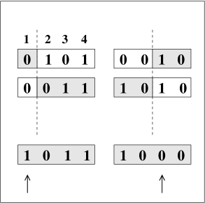
FIG. 1.: Production of gametes. Each pair of bit-strings is cut at a random position and recombined. Mutations are then introduced at random positions in both parts (arrows). For the age-structured part only bad mutations are allowed, while for the non-structured part, both back and forward mutations can randomly occur.

At every iteration, females with age $\geq R$, the minimum reproductive age, search for a partner also with age $\geq R$ to breed, and produce offspring with a birth rate $b$. The offspring genome is constructed by crossing, recombination and mutation, as illustrated in Figure 1. The genome of the mother is cut at a random position and two random complementary pieces are joined to form a female gamete. Deleterious mutations ($0\rightarrow 1$) at random positions are then introduced, with a mutation rate $m$. The same process occurs with the father’s genome and the union of the two gametes completes the offspring genome. In this part of the genome only deleterious mutations may appear, since they are 100 times more frequent than the backward mutations [30]. In this case, if the randomly chosen bit of the parent genome is already one, it remains one in the offspring genome (no mutation occurs). On the other hand, if the chosen bit is zero, it is set to one in the offspring genome.

B Phenotypic Trait, Spatial Lattice and Ecology.

The second pair of bit-strings of each genome is translated into some phenotypic characteristic of the individual [17], as, for instance, its size. This part also suffers crossing and recombination with mutations (Fig. 1). However, for this part both good and bad mutations are allowed ($0\rightarrow 1$ and $1\rightarrow 0$), with a rate $m_{p}$. Moreover, 16 of the 32 bit-positions are dominant and 16 are recessive. The effective number of bits 1, taking into account the dominance, corresponds to a given phenotypic characteristic. This number, which we call the phenotype number $n$, is an integer between zero and 32. For example, we may consider that small values of $n$ correspond to small sized individuals, while large values of $n$ denote big ones.

The individuals are distributed on a two dimensional square lattice. They move at every iteration, with a rate $m_{m}$, to a randomly chosen less or equally populated nearest neighboring site. If all nearest neighbors sites are more populated than the current individual’s site, the movement is not carried out. This strategy guarantees a fast and balanced distribution of individuals over the whole landscape. The reproductive females select their mating partners randomly from the reproductive males localized at the same or at a nearest neighbor site. Reproduction between different phenotypes is not forbidden. Offspring are distributed into empty nearest neighboring sites. If there is no empty site, the offspring is not produced. In this way the population size is controlled by the size of the lattice [31], and there is no need to use the random killing Verhulst factor, present in the traditional version of the Penna model to avoid unlimited population growth.

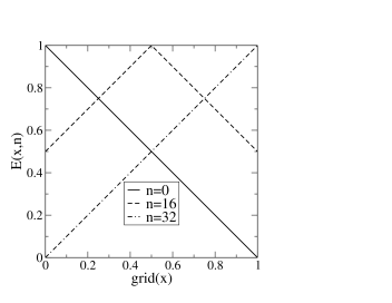
FIG. 2.: Behavior of the ecological function (or probability to die according to x-position and phenotype) $E(x,n)$. Individuals with high or low $n$ survive better on opposite sides of the lattice whereas the ones with intermediate phenotype numbers have a higher death probability everywhere.

The interaction between phenotypic trait and geographical position on a square lattice of linear size $L$ is given by:

$$E(x,n)=S\cdot\left(1-\left|g(x)-\frac{n}{32}\right|\right),$$ (1)

which we call the ecological function. It gives the probability of an individual dying, at every iteration, depending on its x-position and phenotype number. The parameter $S$ is the strength of the interaction and varies between zero and one. The larger the value of $S$ is, the stronger the selection pressure acting on the individuals. The coordinate function is given by $g(x)=\frac{x}{L-1}$, where the coordinate $x$ is an integer between zero and $L-1$. For extreme phenotypes with $n=0$, the perfect region in which to live corresponds to $x=L-1$ where $E(L-1,0)=0$, while for extreme phenotypes with $n=32$ the perfect region corresponds to $x=0$. Individuals with intermediate phenotypes also live better at the extremes of the lattice, but are less fitted than those with extreme phenotypes living in the correct extreme of the lattice. Figure 2 illustrates the ecological function behavior for three different values of $n$.

III Results

In this section we describe the relevant features of speciation found with our simulations, that is, we focus on the interaction between phenotypic trait and the lattice. For results of the traditional sexual Penna model with Verhulst factor or on a lattice we refer to [26] and [31], respectively.

The fixed parameters that we adopt in the simulations are:

i) Threshold number of genetic diseases $T=3$;

ii) Minimum reproductive age $R=8$;

iii) Birth rate $b=4$;

iv) Rate of bad mutations in the chronological genome $m=1$;

v) Number of dominant positions in the chronological genome $D=5$.

vi) Mutation rate of the phenotypic trait $m_{p}=0.15$ or $m_{p}=0.2$.

vii) Number of dominant positions in the phenotypic trait $D_{p}=16$.

The relevant parameters for speciation are the movement rate $m_{m}$, the lattice size $L$ and the strength $S$ of the environmental pressure.

We start the simulations with all the genomes randomly filled with zeroes and ones, and all individuals randomly distributed on the lattice. In order to reach a genetically stable initial population, we run the simulations without any ecological function for 1,000 iterations. During this period the dynamics of the population is neither affected by the phenotype numbers nor by the lattice positions of the individuals. The initial distribution of the phenotype numbers is regulated solely by the mutations, and shows a Gaussian behavior (central curve of Fig. 3).

After these transient steps, the ecology is abruptly changed by setting the ecological function as an additional death probability. Disruptive selection driven by the ecology leads to a better survival of individuals with high and low phenotype numbers, depending on their current positions on the lattice. Three different situations, described below, can be observed, where the environmental pressure and the movement rate are the crucial parameters.

i) At low selection pressures ($S$ small), and independently of the movement rate, the distribution of the phenotype numbers remains unaltered (Gaussian). The population decreases slightly at intermediate positions on the $x$–direction, but during the entire simulation individuals stay in contact over the whole lattice. Gene flow prevents disruptive selection from dividing the system into two sub-populations.

ii) For intermediate selection pressures and movement rates ($m_{m}\sim 1.0$), shortly after turning disruptive selection on, the system reaches an extremely dynamical state where fluctuations may or may not drive the system to divergence. In the cases where speciation does not occur, the adaptation of the phenotypes on one of the lattice sides is faster and gene flow forces the individuals on the other side to adapt themselves to the opposite phenotype (dashed-line with stars in Fig. 3).

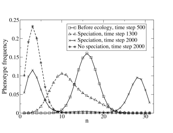
FIG. 3.: The evolution of phenotypic frequency (given by the second pair of bit-strings) versus time. The same set of parameters may or not yield speciation for different random seeds. The central curve (solid line, squares) correspond to the distribution of phenotype numbers before switching on the ecological function (t = 1,000 time-steps). The final distribution when speciation occurs is given by the double-peaked distribution (solid line, crosses). The dashed line with stars corresponds to the final distribution for a case where speciation has not occurred; the dashed line with triangles shows the intermediary distribution in the course of speciation. The parameters: $S=0.24$, $m_{m}=0.99$ and $m_{p}=0.2$.

When phenotypic adaption is balanced, the distribution of phenotype numbers bifurcates. Figure 3 shows that even in the case of speciation, the phenotypic distribution usually drifts away from symmetry before bifurcating, but the final and stable state corresponds to two populations with different phenotypes. We emphasize that during the speciation process the whole population stays in contact and gene flow can not be neglected as in allopatric speciation.

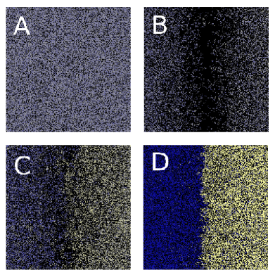
FIG. 4.: Illustration of the phenotype distribution on a $500\times 500$ lattice. The parameters are $m_{m}=0.9$, $S=0.25$ and $m_{p}=0.1$. Black sites are empty. The colors indicate the average value of the phenotype numbers (between yellow and blue). Without disruptive selection, the initial population is homogeneously distributed over the whole lattice (A). When the ecological function is turned on the population is divided into two regions with weak contact (B). Selection prefers different phenotypes with respect to the horizontal location of the individuals and adaptation proceeds (C). Fluctuations decide if the final result is speciation or if it is a single population with phenotypically similar individuals. In case of speciation, two phenotypically different populations can be easily distinguished, each one occupying one side of the lattice (D).

Figure 4 shows the typical spacial distributions of the phenotypes at four different moments of the simulations. Initially, the population is homogeneously distributed over the whole lattice. As soon as the new ecology is turned on, almost all individuals occupying the central x-positions of the lattice die, and the population becomes temporarily divided into two similar groups, with weak contact between them. When the adaptation process of the extreme phenotypes starts, offspring with intermediate phenotype numbers continue to be produced. As the adaptation proceeds, competition with the more fitted extreme phenotypes makes the intermediate ones disappear. Finally, when speciation occurs, each half of the lattice becomes mostly occupied by one of the two extreme phenotypes, respectively. The number of iterations needed to reach the final distribution is about 5000, which corresponds to 625 generations. However, we would like to emphasize that we have run our simulations for up to 100.000 time-steps, to be sure we were obtaining stable distributions.

The final result of a simulation where no speciation occurred, using the same parameters as in Figure 4 but with another initial random seed, is illustrated in Figure 5. In this case only one of the extreme phenotypes remains.

iii) Low movement rates or very high selection pressures prevent speciation events. In both cases a great part of the population dies out at the time when the ecological function is set. Fluctuations dominate divergent adaptation and the initial Gaussian distribution of phenotypes moves to one of the extremes.

FIG. 5.: Another random seed has driven the system to the case of no speciation. One of the two sub-populations randomly dominates and finally occupies the whole lattice. In this case, the worst region of the lattice for the winning extreme phenotype to survive (left side in this figure) remains less populated than the rest of the lattice, that is, the occupation is not uniform.

It is important to say that for small population sizes fluctuations seem to always prevent speciation, independently of the movement rate: no speciation events have been obtained for lattice sizes smaller than $L=150$.

Concerning the selection pressure, it was also found by Doebeli [32] that very high values of $S$ prevent speciation.

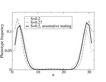
FIG. 6.: Comparison of the final states of the phenotype distributions for different values of the parameter $S$. The stronger the ecology is, the less frequent are the hybrids. Assortative mating leads to the non-existence of hybrids, depicted by the thick curve where $d=10$. The movement rate $m_{m}=0.9$ and the mutation rate related to the phenotype is $m_{p}=0.15$.

In order to study the effect of sexual selection in our simulations, we introduce the assortative mating strategy used in [29] to prevent the mating of extreme phenotypes (prezygotic isolation). We measure the absolute difference of the phenotype numbers of both male and female, before mating. If the difference is larger than $d$, they can not reproduce. If there is no appropriate male among the nearest neighbors, no offspring is produced. Figure 6 shows the final phenotype distributions for different strengths $S$ of the ecological function, in cases where speciation occurred. We compare different results using random mating to one where assortative mating is used, with $d=10$. It can be seen that assortative mating completely prevents the production of hybrids with phenotype numbers around 16. Additionally, the occurrence of speciation is controlled by the parameter $d$, as in [29]. Very small values of $d$ ($d<8$) prevent speciation due to the lack of genetic diversity, which is an important ingredient for the distribution of phenotype numbers to bifurcate.

In Figure 7 we show the histogram of the fraction of the population that dies at a given age, for different phenotype numbers. The majority of the hybrids die at low ages and do not generate offspring. These hybrids present low viability and thus characterize a speciation process [12].

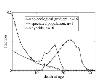
FIG. 7.: Life span for different phenotype numbers. Most of the hybrids die at low ages.

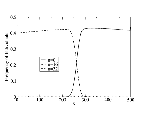
FIG. 8.: Frequency of individuals with a given phenotype number for each position $x$ of the lattice, averaged over the last 10,000 time steps.

A cline is defined as a gradient in a measurable character. Relative to the dispersal rate of a species, the slope of a cline between regions is indicative of the extent to which the inhabitants have differentiated. A steep cline means sharp differentiation while a gentle cline means indistinct divergence between areas [21]. In our case we choose the phenotype number, $n$, as the measurable character. Figure 8 shows the fraction of individuals with $n=0$, $n=16$ and $n=32$ at each position $x$ of the lattice. A steep cline can be observed for the $n=0$ and $n=32$ populations, as well as the almost disappearance of the hybrids with $n=16$.

FIG. 9.: Final state of the simulation without disruptive selection. No speciation occurs.

A common outcome in Nature consists of phenotypically distinguishable forms at geographic extreme regions and inter-grading hybrid forms in between. In our case disruptive selection due to the ecological function in eq.(1) prevents such a scenario. However, using the following ecological function:

$$E(x,n)=S\cdot\left|g(x)-\frac{n}{32}\right|,$$ (2)

hybrids are now favored and so do not disappear, that is, there is no speciation as shown in figures 9 and 10. From fig. 9 we can observe that the mean value of the phenotypes changes continuously with the geographic position $x$ and there is no sharp separation between the two extreme regions. It is important to say that in using eq.(2) speciation is not obtained even if assortative mating is included (fig. 10).

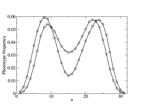
FIG. 10.: Final phenotype distribution for simulations with the ecology function eq.(2). Even for a simulation with assortative mating gene flux prevents speciation.

IV Discussion

As reported by Gavrilets [33] the dynamics of parapatric speciation is very fast (less than 1,000 generations) and is independent of the mutations rate $m_{p}$ of the phenotypic trait. We have made some simulations with smaller mutation rates and the time needed to reach a steady state did not increase for $m_{p}>0.0001$.

In our model the ecological function must be disruptive, i.e. individuals with intermediate phenotypes have to be discriminated. In a non–disruptive ecology individuals of all phenotypes can adapt to their local environments and hybrids evolve easily at intermediate x-positions. At the end of the simulations individuals of all phenotypes populate the lattice. If the selection against individuals with intermediate phenotype numbers is not strong enough, only an unstable polymorphism appears: The two subpopulations coexist with large gene flux between them until one of them completely dominates and uniformly occupies the whole lattice.

Different from other speciation models, ours allows fluctuations of all quantities, which hinders adaptation and the division of the system into two different phenotypic populations, even for intermediate values of the selection pressure. This could explain the not so frequent occurrence of speciation in Nature, where many environmental factors act on the different population quantities, like the phenotypic distribution, and where fluctuations of these quantities are ubiquitous. Even if the conditions are optimal, speciation remains a statistical event (that is, for ten different initial random seeds, about five result in speciation and the other five result in an unimodal phenotypic distribution). Speciation is observed frequently for large lattices, where the phenotype distributions fluctuate less. Our results suggest that parapatric speciation occurs preferably in cases where a large population undergoes a sudden disruptive selection over large geographical distances compared to the range of individuals movements.

We have studied the effect of assortative mating in our model, but the final results obtained were nearly the same as those using random mating, although the rule of  [29] increases the probability of speciation occurring. Even without assortative mating, only a very small number of hybrids is born (less than 1% of the total population) due to the small range of the mating region (only between nearest neighbors individuals). Moreover, Figure 7 shows that these hybrids die mainly at low ages and do not produce offspring, which can be interpreted as a form of postzygotic reproductive isolation. In this way a small gene flow does not prevent speciation in this parapatric scenery, even without assortative mating. Models with small population sizes or mating over large geographical distances need assortative mating in order to obtain speciation [29, 32].

V Conclusions

We present an individual-based model for parapatric speciation, where individuals with different phenotypes are distributed on a spatial lattice. Individuals may die due to genetic diseases or due to a competition for resources that depends on their phenotypes and on their geographical positions. Mating occurs only between next nearest neighbors. Surprisingly, even when considering random mating, fluctuations due to a disruptive selection may drive the system to speciation. On the other hand, under very strong disruptive selection, fluctuations prevent speciation to occur.

In fact, the importance of our approach is that it allows fluctuations in nearly all quantities. Physicists are very conscious about the importance of fluctuations in physical systems, mainly when they present a phase transition, which can be regarded as a process of bifurcation from a single phase (for instance, gas) into a state where two different phases coexist (liquid and vapor). The simplest, naive strategy to deal with such a phenomenon is the mean-field approach, in which the influences of the many units of the system over a particular one is replaced by an average influence or an “average unity”, disregarding completely all possible fluctuations. However, this kind of treatment always gives wrong values for the critical exponents and sometimes signals the existence of a phase transition when it does not exist, since the fluctuations that would prevent the transition to occur are omitted [34].

The speciation process is also a problem of bifurcation and mean-field approaches are widespread (see for instance [7, 8]). Again, they certainly give the wrong speciation velocity (related to critical exponents) and may predict a speciation event when it does not exist. An example of mean-field approach as applied to genetic evolution follows. Instead of considering the genetic features of each individual separately, in a given generation, one considers the genetic frequency distribution of the whole population and imposes some rule for its time evolution from one generation to the other. Indeed, in this case, the genetic information of the whole population is collapsed into a single “average individual”, characterizing the above mentioned mean-field approach. On the other hand, our model considers each individual separately, and so does not ignore fluctuations. That is why speciation may or not appear depending on the initial random seed, for the same set of parameters.

REFERENCES

- [1] E. Mayr, Animal Species and Evolution (Harvard Univ. Press, 1963).
- [2] S. Gavrilets, Nature 403, 886 (2000).
- [3] R. Lande, Evolution 36, 213 (1982).
- [4] F. Turner, G. and M. Burrows, Proc. R. Soc. Lond. B 260, 287 (1995).
- [5] G. van Doorn, A. Noewst, and P. Hogeweg, Proc. R. Soc. Lond. B 265, 1915 (1998).
- [6] M. Higashi, G. Takimoto, and N. Yamamura, Nature 402, 523 (1999).
- [7] A. Kondrashov and F. Kondrashov, Nature 400, 351 (1999).
- [8] U. Dieckmann and M. Doebeli, Nature 400, 354 (1999).
- [9] K. Luz-Burgoa, S. Moss de Oliveira, J. S. Sá Martins, D. Stauffer, and A. O. Sousa, Braz. J. Phys. 33, 623 (2003).
- [10] M. E. Arnegard and A. S. Kondrashov, Evolution 58, 222 (2004).
- [11] C. R. Almeida and F. V. de Abreu, Evol. Ecol. Res. 5, 730 (2003).
- [12] A. H. Porter and N. A. Johnson, Evolution 56, 2103 (2002).
- [13] W. R. Rice and E. E. Hostert, Evolution 47, 1637 (1993).
- [14] U. K. Schliewen, D. Tautz, and S. Pääbo, Nature 368, 629 (1994).
- [15] D. Schluter, Science 3266, 798 (1994).
- [16] S. Via, Trends Ecol. Evol. 16, 381 (2001).
- [17] J. S. Sá Martins, S. Moss de Oliveira, and G. A. de Medeiros, Phys. Rev. E 64, 021906 (2001).
- [18] S. Gavrilets, Fitness landscapes and the origin of species (Princeton University Press, 2004).
- [19] J. Coyne and H. Orr, Speciation (Sinauer Associates, 2004).
- [20] M. Slatkin, Genetics 75, 733 (1973).
- [21] J. A. Endler, Science 179, 243 (1973).
- [22] M. Kirkpatrick and N. H. Barton, Am. Nat. 150, 1 (1997).
- [23] N. Sanderson, Evolution 43, 1223 (1989).
- [24] T. Day, Evolution 54, 715 (2000).
- [25] T. J. P. Penna, J. Stat. Phys. 78, 1629 (1995).
- [26] S. Moss de Oliveira, P. M. C. de Oliveira, and D. Stauffer, Evolution, Money, War and Computers (Teubner, 1999).
- [27] D. Stauffer, P. M. C. de Oliveira, S. Moss de Oliveira, T. J. P. Penna, and J. S. Sá Martins, An. Acad. Bras. Ci. 731, 15 (2001).
- [28] A. O. Sousa, Eur. Phys. J. B 39, 521 (2004).
- [29] S. Gavrilets, Trend Ecol. Evol. 12, 307 (1997).
- [30] P. Pamilo, M. Nei, and W. H. Li, Genet. Res. 49, 135 (1987).
- [31] D. Makowiec, Physica A 289, 208 (2001).
- [32] M. Doebeli and U. Dieckmann, Nature 421, 259 (2003).
- [33] S. Gavrilets, H. Li, and M. Vose, Proc. R. Soc. Land. B 265, 1483 (1998).
- [34] R. Baxter, Exactly Solvable Models in Statistical Mechanics (Academic Press, 1982).