Phase transition in a mean-field model for sympatric speciation

Abstract

We introduce an analytical model for population dynamics with intra-specific competition, mutation and assortative mating as basic ingredients. The set of equations that describes the time evolution of population size in a mean-field approximation may be decoupled. We find a phase transition leading to sympatric speciation as a parameter that quantifies competition strength is varied. This transition, previously found in a computational model, occurs to be of first order.

1 Introduction

The dynamics that generate the rich and diverse structure of the living world is still one of the greatest puzzles in science. Why and how the primitive living organisms gave birth to the immense variety of species in our environment is still a matter of debate and research to our days. The theory of biological evolution, the paradigm that guided the rapid growth of our knowledge about the microscopics (e.g. the behaviour of individuals in a population) of life and the development of all the dazzling techniques and possibilities of genetical engineering, has yet to answer some simple and rather basic questions. One of these stands out as a crucial difficulty: the issue of sympatric speciation.

If a single-species population is somehow split into two separate groups - by the establishment of some geographical barrier, say - uncorrelated genetic drift in these non-mating populations may eventually lead to differentiation. This process is called allopatric speciation and is reasonably well understood. The same cannot be said about the branching of a single population into two distinct species without the appearance of an external barrier dividing the original group: sympatric speciation. Until recently, the possibility of such a process was still under debate, but observations of micro-evolution [1] and the development of theoretical frameworks [2, 3, 4] have established it as a valid conjecture in the last years, turning sympatric speciation into one of the favourite themes of research in modern evolutionary theory [5, 6, 7].

A variety of theoretical models have been proposed to explain sympatric speciation, from analytical mean-field type ones to to more realistic individual-based models. Computational representations based on variations of the Penna model for biological ageing [8], popular amongst physicists working on the statistical mechanical aspects of evolutionary theory, belong to this latter class. Previous work on such representations have shown that sympatric speciation appears when driven by a change in the character of the distribution of ecological resources, as suggested by some biologists [3]. From this perspective, sympatric speciation appears as a transition between two different organisations of some population. In our present work, we develop a variation that allows a mean-field approximation with analytical solution, in which the nature of this transition may be further discussed.

The computational model has intra-specific competition, mutations and assortative mating as its sole ingredients. The mean-field approximation leads to a set of simple equations that reproduces some of the features of individual-based models, and whose solutions show a clear signature of the above mentioned phase transition.

2 The computational model

We take as starting point the sexual version of the Penna model, as described for instance in refs. [9, 10]. In addition to the age-structured pair of bit-strings that represents the genome for purposes of ageing analysis, each individual carries an extra pair of non-structured bit-strings of 32 bits each, that encodes a genetically acquired phenotype trait, as already published in ref. [11]. This extra pair of genetic material is inherited with the same dynamics of the age-structured pair, involving a meiotic cycle with crossing and recombination of each parent’s bit-strings. The trait for a particular individual is obtained by counting the number of loci in the non-structured pair where the allele $1$ is either homozygous or dominant, and is an integer in the interval $[0,32]$ which determines the individual’s survival probability and its mating preferences. The positions where the allele $1$ is dominant are chosen randomly at the beginning of the simulation and are the same for all individuals. According to this number, the population is divided into three groups (subpopulations). We will follow the dynamical evolution of the size of the three subpopulations independently ($P_{1}$ for the one with small values of the phenotype trait, $P_{2}$ for the one with large values, and $P_{i}$ for the intermediate one). The survival probability is $1-V$, where $V$ is the so-called (modified) Verhulst factor. This factor has a resource-size parameter, the carrying capacity $C$, and represents a mean-field competition for the ecological resources of the environment. It has a different value for each one of the three subpopulations, representing different levels of competition for those resources:

$$V_{P_{1,2}}=\frac{P_{1,2}+P_{i}}{C},\,\,\,V_{P_{i}}=\frac{x(P_{1}+P_{2})+P_{i}}{C}$$ (1)

where we set $C=100,000$. The intermediate subpopulation $P_{i}$ competes with a fraction $x$ of the sum of the subpopulations with extreme values of the phenotype trait, and this fraction will drive the speciation phase transition. Each of the subpopulations $1$ and $2$ competes only with itself and with the intermediate one. This variation of the Verhulst factor has previously been used in a study of sympatric speciation in food webs [12]. A genetic trait, encoded by a single bit and subject to mutation, determines female selectivity in mating. This trait is initially set to zero: every female selects a mating partner randomly. Observe that due to mutations the offspring of a selective female may be non-selective and vice-versa. Mating preference also depends on the value of the phenotype trait. A selective female of population $P_{1}$ or $P_{2}$ chooses to mate, among a set of $A$ males from its own subpopulation, the one with the most extreme value of the phenotype trait. A selective female of population $P_{i}$ chooses randomly to act as one of the above. Any non-selective female mates randomly. The number $A$ of available males is a measure of the female’s selectivity degree: the larger $A$ is, more selective is the female.

3 Results of the computational model

We focus on the identification of the phase transition already mentioned. Fig. 1 compares the final states of simulations carried out with extreme values of $x$ with the one at the transition point $x=0.5$. In all cases, $A=50$, the mutation probability at birth of a locus of the phenotype trait is $0.01$, and total time equals $100,000$ MC steps. Speciation is well observed for $x=1$, where complete reproductive isolation leads to the absence of gene flux between the extreme populations and consequently to the extinction of intermediate phenotypes. Genetic variety and gene flux increases crucially at the transition point $x=0.5$. The signature of the transition is the abrupt change of the fraction of selective females in the population, $N_{s}$, which acts as an order parameter. In a single species environment, this fraction is close to $0$, and it increases to $1$ with the event of speciation. As the control parameter $x$ is increased from $0$, the order parameter $N_{s}$ undergoes a clear transition, as seen in fig. 2. A similar transition also occurs if a selective female chooses the mating partner that most closely matches her own phenotype trait, instead of the most extreme one [13, 14, 15], showing that the extreme mating strategy is not crucial.

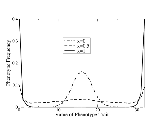
Figure 1: The frequency of individuals as a function of the value of the phenotype trait in the final state of the simulations, for some values of the competition degree $x$.

At the transition point the fluctuation of $N_{s}$, measured as the mean deviation of multiple realizations of the simulations, presents a peak. As the selectiveness parameter $A$ is increased, so does the steepness of the transition. The transition can also be seen in the behaviour of $P_{1}$, $P_{i}$, $P_{1}+P_{2}+P_{i}=P_{total}$, and $P_{1}-P_{i}$. In fact, we will single out this last quantity to signal the occurrence of speciation, as commented below. A full description of the nature of the sympatric speciation transition as obtained via the computational microscopic model is being published elsewhere [13, 14, 15].

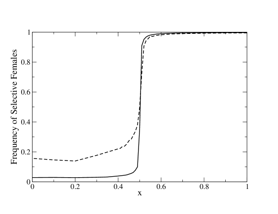
Figure 2: Results of the computational model showing the fraction of selective females for the values $A=50$ (solid line) and $A=3$ (dashed line) as a function of $x$. Speciation occurs when this fraction reaches a value close to $1$.

4 Mean-field approximation

A mean-field approximation to the microscopic model can be cast under the form of a system of coupled differential equations. Dynamics of all three subpopulations are frequency-dependent; for the intermediate subpopulation, we add a competition for ecological resources with a fraction $x$ of each of the extreme-sized ones, as done in the microscopic model. The system of equations is thus:

$$\frac{dP_{1}}{dt}=(a-b)P_{1}+bP_{i}-\frac{1}{C}(P_{1}+P_{i})P_{1}$$ (2)

$$\frac{dP_{2}}{dt}=(a-b)P_{2}+bP_{i}-\frac{1}{C}(P_{2}+P_{i})P_{2}$$ (3)

$$\frac{dP_{i}}{dt}=(a-2b)P_{i}+bP_{1}+bP_{2}-\frac{1}{C}(xP_{1}+xP_{2}+P_{i})P_{i}$$ (4)

The parameter $a$ describes the birth rate, and is the same for all subpopulations. In order to characterise the exchange parameter $b$, we have to envision one process before as well as another one after crossing and recombination. In the first, the bits of the phenotypic trait are reshuffled by crossing-over of the gametes of both parents, a process that can lead to drastic changes in the value of this trait. The amount of this change is controlled by the number of males ($A$) each female will choose from as mating partner, as well as by the number of selective females in the population. Additionally, mutations may change the number that characterises an individual’s trait. This last process is independent from the reshuffling and thus can be described by a constant value. These two processes are rather difficult to include in a mean-field model. For simplicity, we chose to model them by postulating that each subpopulation with extreme phenotype generates a fraction $b$ of its offspring with a phenotype of the intermediate subpopulation. The latter looses a fraction of $2b$ offspring to the extreme subpopulations. The parameter $b$ synthesises the combined effect of the mutation rate and of the degree of assortativity in the mating process, which should be proportional to the reciprocal value of $A$. Thus, even if assortative mating is maximum, the parameter $b$ cannot be set to zero, since we still have to model the effect of mutations. We will refer to $b$ as a parameter of female selectivity in the following, keeping in mind that it also contains the effect of mutations. Competition is introduced through the density-dependent Verhulst factor, to which the parameter for the carrying capacity $C$ is related.

Because of the intrinsic symmetry of the model, the subpopulation with a small value for the phenotype trait ($P_{1}$) has a dynamical evolution equivalent to the one with a high value for the trait ($P_{2}$). In each of these, the time evolution of its size depends on its current value as well as on the size of the intermediate subpopulation. We assume, as an approximation, that they are equal at all times, and set $P_{1}=P_{2}$ in eq. (2):

$$\frac{dP_{i}}{dt}=(a-2b)P_{i}+2bP_{1}-\frac{1}{C}(2xP_{1}+P_{i})P_{i}.$$ (5)

The system of eqs. (2) and (5) can be simplified by the following transformations:

$$f=\frac{1}{4C}(P_{1}+P_{i});\,\,g=\frac{1}{4C}(P_{1}-P_{i});\,\,\epsilon=2x-1,$$ (6)

$\epsilon$ being a control parameter in terms of which the transition is set at $\epsilon=0$. As a result of this transformation, the system of equations now reads:

$$\frac{df}{dt}=af+bg-(\epsilon+4)f^{2}+\epsilon g^{2},$$ (7)

$$\frac{dg}{dt}=(a-3b)g-\epsilon g^{2}-4fg+\epsilon f^{2}.$$ (8)

To look for characteristics of the stationary solutions, which are the fixed points of the differential system, we set the time derivatives to $0$ and obtain a relation between the functions $g$ and $f$:

$$g=-f\frac{4f-a}{4f-a+2b}$$ (9)

The existence of the phase transition in the mean-field approximation is clear in fig. 3, in which the exact and stable solutions for the size of the subpopulations are shown as a function of the new control parameter $\epsilon$. The transition point $\epsilon=0$ separates a region in phase space where the subpopulations still interbreed ($\epsilon<0$) and the intermediate population is large, from another one, in which the subpopulation that results from interbreeding all but vanishes, characterising assortative mating within each of the subpopulations. In the latter, these can now be said to constitute two different non-mating species.

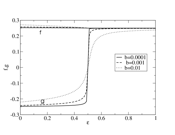
Figure 3: The stable fixed points of the mean-field model for different values of $b$, characterising female selectivity. When $b$ increases, the transition becomes smoother.

Exploration of the parameter space shows that this transition becomes smoother as the selectivity degree parameter $b$ increases, as shown in fig. 3. In all cases, the function $f$ is nearly constant (in fig. 4 compared to the computational model), as can be seen directly from the results of the simulations of the computational model. The latter results also show fluctuations in the values of all subpopulations, as well as in $g$, that peak as the transition point is approached. This is not true for $f$ though, for which the fluctuations are small and do not show any change of behaviour at the transition. The role played by the female selectivity $A$ is equivalent to the corresponding parameter in the mean-field approximation, $b$: an increase in selectivity $A$, corresponding to a decrease in $b$, sharpens the transition.

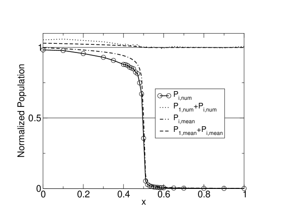
Figure 4: Comparison of the result for $P_{i,num}$ of the computational model ($A=50$) with the mean-field approximation $P_{i,mean}$, fitted with $b=0.001$. The quantity $f\propto P_{1}+P_{i}$ is nearly constant. The horizontal full straight lines are guides to the eyes.

In order to obtain a full characterisation of the transition, and supported by the results of the simulations, we impose $f$ to be some constant from the start, and independent of $\epsilon$. Additionally, we neglect the term $bg$ in eq. (7). The relations $f>0$, $f>g$ as well as $b\ll a$, valid in all cases we have studied, justify this simplification. It is easy to compute the value of $f$ from the differential system at the transition point $\epsilon=0$, $f=\frac{a}{4}$. $f$ can be set constant also because of the following reason: If we add a small perturbation $\delta$ to $f$ in eq. 9 we obtain $g=-\delta\frac{a}{2b}$ with $b\ll a$. We are also left with a single differential equation for $g$,

$$\frac{dg}{dt}=-\epsilon g^{2}-3bg+\epsilon\frac{a^{2}}{16}$$ (10)

with a stationary solution that exhibits symmetry with respect to the transition point:

$$g_{*}=-\frac{3b}{2\epsilon}+\sqrt{(\frac{3b}{2\epsilon})^{2}+(\frac{a}{4})^{2}}.$$ (11)

To establish the validity of these last approximations, we may compare the above result with the stable solution of the full mean-field solution. Fig. 5 shows both results, and compares them to the numerical results. Deviations do exist, but they do not change the qualitative nature of the solutions.

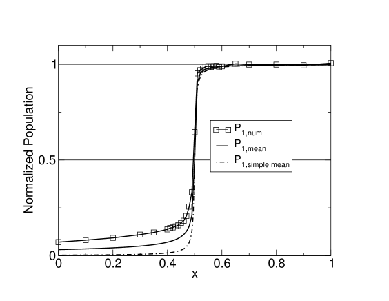
Figure 5: Comparison of the result for $P_{1,num}$ of the computational model ($A=50$) with the mean-field approximations $P_{1,mean}$, fitted with $b=0.001$. The simplified mean-field model $P_{1,simple\,mean}$ also reproduces well the simulations.

We now proceed to obtain the time dependence of the solution. This behaviour could be interpreted as if, after reaching the stationary state, the value of the control parameter was changed; the time behaviour of the solution is then followed as it approaches a new equilibrium. This can be done more easily if we apply the transformation $z=\frac{1}{g-g_{*}}$ to get the equation for $z(t)$,

$$\frac{dz}{dt}=\epsilon+\sqrt{9b^{2}+\epsilon^{2}\frac{a^{2}}{4}}\cdot z=\epsilon+rz$$ (12)

with a time-dependent solution for $g(t)$ given by

$$g(t)=-\frac{r}{\epsilon}\cdot\frac{1}{1-\phi e^{rt}}+g_{*}$$ (13)

The parameter $\phi$ depends on the initial condition. If it has a value in the interval $0<\phi<1$, then $g(0)<g-2f=-P_{1}-3P_{i}$, which lies beyond the range of $g$. The analytical solution is a very good approximation to the result of the simulations, yielding the same exponential behaviour.

If we impose the condition that $f$ has a constant value, still at the transition point $\epsilon=0$, then the solution for $g(t)$ is $g(t)=g_{0}e^{-3bt}$, whereas the full solution, neglecting only the term $bg$ is given by

$$f(t)=\frac{a}{\beta e^{-at}+4},\,g(t)=g_{0}e^{-3bt}\frac{1}{\beta e^{-at}+4}$$ (14)

where $g_{0}$ and $\beta$ depend on the initial conditions. Unfortunately, the exponential decay we obtain in the analytical solution does not allow us to determine a precise relation between the selective strength parameters of the microscopic and mean-field models, due to too high a level of fluctuations.

5 Conclusions

The microscopic models for the study of sympatric speciation, and in particular those based on variations of the Penna model, have proven their value yielding a number of interesting results and providing some background for a testing ground of evolutionary theories. We have here reported that one of those versions admits a mean-field approximation with an analytical solution that closely matches the results of the simulations. This new tool can be helpful in the characterisation of sympatric speciation as an out-of-equilibrium phase transition, and help in the study of the statistical properties of the system on both sides of that transition. The thermodynamical nature of this transition may also be analysed in this context, as well as the character of the fluctuations and the quantitative properties connected to the transition point. Work on these lines is already in progress.

References

- [1] M.L. Friesen et al., Evolution 58, 254 (2004).
- [2] R. Lande, Proc. Natl. Acad. Sci. 78, 3721 (1981).
- [3] A. S. Kondrashov, F. A. Kondrashov, Nature, 400, 351 (1999).
- [4] S.S. Chow et al., Science 305, 84 (2004).
- [5] M. Turelli, M. H. Barton, J. A. Coyne, Trends Ecol. Evol. 16, 330 (2001).
- [6] S. Gavrilets, Fitness landscapes and the origin of species (Princeton University Press, 2004).
- [7] J. Coyne and H. Orr, Speciation (Sinauer Associates, 2004).
- [8] T.J.P. Penna, J. Stat. Phys. 78, 1629 (1995).
- [9] S. Moss de Oliveira, D. Alves, and J.S. Sá Martins, Physica A 285, 77 (2000).
- [10] S. Moss de Oliveira, P. M. C. de Oliveira, and D. Stauffer, Evolution, Money, War and Computers (Teubner, 1999).
- [11] J.S. Sá Martins, S. Moss de Oliveira, and G.A. de Medeiros, Phys. Rev. E 64, 021906 (2001).
- [12] K. Luz-Burgoa, Tony Dell, Toshinori Okuyama, q-bio.PE/0502010; also in Contribution to the Proceedings of the Complex Systems Summer School 2004, organized by the Santa Fe Institute (2004).
- [13] K. Luz-Burgoa, Doctoral Thesis, UFF, q-bio.PE/0504006 (2005);
- [14] K. Luz-Burgoa, V. Schwämmle, S. Moss de Oliveira and J.S. Sá Martins, submitted (2005);
- [15] K. Luz-Burgoa, S. Moss de Oliveira, J.S. Sá Martins, D. Stauffer, and A.O. Sousa, Braz.J.Phys. 33, 623 (2003).