Allostery in a Coarse-Grained Model of Protein Dynamics

Abstract

We propose a criterion for optimal parameter selection in coarse-grained models of proteins, and develop a refined elastic network model (ENM) of bovine trypsinogen. The unimodal density-of-states distribution of the trypsinogen ENM disagrees with the bimodal distribution obtained from an all-atom model; however, the bimodal distribution is recovered by strengthening interactions between atoms that are backbone neighbors. We use the backbone-enhanced model to analyze allosteric mechanisms of trypsinogen, and find relatively strong communication between the regulatory and active sites.

A major challenge of molecular biology is to understand regulatory mechanisms in large protein complexes that are abundant in multi-celluluar organisms. To make simulation of such complexes computationally feasible, coarse-grained models have been developed, in which a subset of the atoms in the complex are used to simulate the large-scale motions. However, principled methods to quantify and optimize the accuracy of coarse-grained models are currently lacking.

In one common coarse-graining method, an all-atom model is simplified by considering effective interactions among a subset of the atoms (e.g., just the alpha-carbons). The usual criterion for model accuracy is the ability of a model to reproduce atomic mean-squared displacements (MSDs). However, MSDs are just one aspect of protein dynamics – a stricter criterion for the accuracy of a coarse-grained model is the similarity between the configurational distributions of the selected atoms in the coarse-grained and all-atom models. Such a criterion is also biologically relevant, in part because the conformational distribution is a key determinant of protein activity Frauenfelder and Wolynes (1985).

One useful measure of the difference between conformational distributions is the Kullback-Leibler divergence $D_{\bf x}$ (see definition below) Kullback and Leibler (1951); Ming and Wall (2005). Recently, an analytic expression for $D_{\bf x}$ was obtained for harmonic vibrations of a protein-ligand complex both with and without a protein-ligand interaction Ming and Wall (2005). Here we show how an equivalent expression may be applied to refine a coarse-grained model of protein dynamics. To use the expression for $D_{\bf x}$ requires the marginal probability distribution of a subset of the atoms in a protein, which we calculate in the harmonic approximation. We then apply the equations to refine an anisotropic elastic network model (ENM) Atilgan et al. (2001) of trypsinogen dynamics with respect to an all-atom model calculated using CHARMM Brooks et al. (1983). The unimodal density-of-states distribution of the ENM disagrees with the bimodal distribution obtained from the all-atom model; however, the bimodal distribution is recovered by strengthening interactions between atoms that are backbone neighbors. Finally, the backbone-enhanced elastic network model (BENM) is used to analyze allosteric mechanisms of trypsinogen, revealing relatively strong communication between the regulatory and active sites.

Let $P({\bf x})$ be the probability distribution of the $3N$ atomic coordinates ${\bf x}=(x_{1},y_{1},z_{1},\ldots,x_{N},y_{N},z_{N})$ of a molecular model in the harmonic approximation. Let ${\bf x}=({\bf x}_{1},{\bf x}_{2})$, where ${\bf x}_{1}$ is the $3N_{1}$ coordinates of a subset of atoms of interest, and ${\bf x}_{2}$ is the $3N_{2}$ coordinates of the remaining atoms. We are interested in calculating the marginal distribution $P({\bf x}_{1})$:

$$P({\bf x}_{1})=\int d^{3N_{2}}{\bf x}_{1}\,P({\bf x}_{1},{\bf x}_{2}).$$ (1)

We now calculate $P({\bf x}_{1})$ in a model of molecular vibrations. Consider a harmonic approximation to the potential energy function $U({\bf x})$, where ${\bf x}$ is the deviation from an equilibrium conformation ${\bf x}_{0}$:

$$U({\bf x}+{\bf x}_{0})\approx U({\bf x}_{0})+{1\over 2}{\bf x}^{\dagger}{\bf H}\,{\bf x}.$$ (2)

The matrix ${\bf H}$ is the Hessian of $U$ evaluated at ${\bf x}_{0}$: $H_{ij}|_{{\bf x}_{0}}=\partial^{2}U/\partial x_{i}\partial x_{j}|_{{\bf x}_{0}}.$ We assume a Boltzmann distribution for $P({\bf x})$, and ignore solvent and pressure effects:

$$P({\bf x})=Z^{-1}e^{{-{\bf x}^{\dagger}{\bf H}\,{\bf x}}\over{2k_{B}T}}=(2\pi k_{B}T)^{-3N/2}e^{{-\left|{\bf\Omega}{\bf V}^{\dagger}{\bf x}\right|^{2}}\over{2k_{B}T}}\prod_{i=1}^{3N}\omega_{i},$$ (3)

where $Z$ is the partition function, $k_{B}$ is Boltzmann’s constant, $T$ is the temperature, the elements of the matrix $\left|{\bf\Omega}\right|^{2}={\rm diag}(\omega_{1}^{2},\ldots,\omega_{3N}^{2})$ are the eigenvalues of ${\bf H}$, and the columns of the matrix ${\bf V}$ are the eigenvectors of ${\bf H}$. To calculate $P({\bf x}_{1})$ we define the submatrices ${\bf H}_{1}$, ${\bf H}_{2}$, and ${\bf G}$ as follows:

$${\bf H\,x}=\left(\begin{array}[]{cc}{\bf H}_{1}&{\bf G}\\ {\bf G}^{\dagger}&{\bf H}_{2}\end{array}\right)\left(\begin{array}[]{c}{\bf x}_{1}\\ {\bf x}_{2}\end{array}\right)=\left(\begin{array}[]{ccc}{\bf H}_{1}{\bf x}_{1}&+&{\bf G}{\bf x}_{2}\\ {\bf G}^{\dagger}{\bf x}_{1}&+&{\bf H}_{2}{\bf x}_{2}\end{array}\right).$$ (10)

${\bf H}_{1}$ couples coordinates from ${\bf x}_{1}$; ${\bf H}_{2}$ couples coordinates from ${\bf x}_{2}$; and ${\bf G}$ couples coordinates between ${\bf x}_{1}$ and ${\bf x}_{2}$. Eq. (3) now can be expressed as

$$P({\bf x})=Z^{-1}e^{{-{\bf x}^{\dagger}{\bf H}\,{\bf x}}\over{2k_{B}T}}=(2\pi k_{B}T)^{-3N/2}e^{{-\left|{\bf\bar{\Omega}}{\bf\bar{V}}^{\dagger}{\bf x}_{1}\right|^{2}-\left|{\bf\Lambda}{\bf U}^{\dagger}{\bf x}_{2}+{\bf\Lambda}^{-1}{\bf U}^{\dagger}{\bf G}^{\dagger}{\bf x}_{1}\right|^{2}}\over{2k_{B}T}}\prod_{i=1}^{3N}\omega_{i},$$ (11)

where the diagonal elements of the matrix $\left|{\bf\Lambda}\right|^{2}={\rm diag}(\lambda_{1}^{2},\ldots,\lambda_{3N_{1}}^{2})$ and the columns of the matrix ${\bf U}$ are the eigenvalues and eigenvectors of ${\bf H}_{2}$, and the diagonal elements of the matrix $\left|{\bf\bar{\Omega}}\right|^{2}={\rm diag}(\bar{\omega}_{1}^{2},\ldots,\bar{\omega}_{3N_{1}}^{2})$ and the columns of the matrix ${\bf\bar{V}}$ are the eigenvalues and eigenvectors of a matrix ${\bf\bar{H}}$ defined as

$${\bf\bar{H}}={\bf H}_{1}-{\bf G}{\bf H}_{2}^{-1}{\bf G}^{\dagger}={\bf\bar{V}}\left|{\bf\bar{\Omega}}\right|^{2}{\bf\bar{V}}^{\dagger}.$$ (12)

Eq. (12) is equivalent to an equation independently derived to study local vibrations in the nucleotide-binding pockets of myosin and kinesin Zheng and Brooks (2005). Performing the integral in Eq. (1) leads to the desired equation for $P({\bf x}_{1})$:

$$P({\bf x}_{1})=(2\pi k_{B}T)^{-3N_{1}/2}e^{{-\left|{\bf\bar{\Omega}}{\bf\bar{V}}^{\dagger}{\bf x}_{1}\right|^{2}}\over{2k_{B}T}}\prod_{i=1}^{3N_{1}}\bar{\omega}_{i}.$$ (13)

Now consider the problem of optimal selection of the parameters $\Gamma$ of a coarse-grained model of protein dynamics. Let ${\bf x}_{\alpha}$ be the coordinates of the $N_{\alpha}$ alpha-carbons in an an all-atom model, and ${\bf x}_{\alpha}^{(\Gamma)}$ be the same coordinates in the coarse-grained model. We define the optimal coarse-grained model as the one for which the Kullback-Leibler divergence between $P^{(\Gamma)}({\bf x}_{\alpha})$ and $P({\bf x}_{\alpha})$ is minimal, i.e., for which $\Gamma$ is chosen such that

$$D_{{\bf x}_{\alpha}}^{(\Gamma)}=\int d^{3N_{\alpha}}{\bf x}_{\alpha}\,P^{(\Gamma)}({\bf x}_{\alpha})\ln{P^{(\Gamma)}({\bf x}_{\alpha})\over P({\bf x}_{\alpha})}$$ (14)

is minimal. We previously calculated an analytic expression for equations like Eq. (14) when $P({\bf x}_{\alpha})$ and $P^{(\Gamma)}({\bf x}_{\alpha})$ are both governed by harmonic vibrations Ming and Wall (2005):

$$D_{{\bf x}_{\alpha}}^{(\Gamma)}=\sum_{i=1}^{3N_{\alpha}}\left(\ln{\omega_{i}^{(\Gamma)}\over\bar{\omega}_{i}}+{1\over{2k_{B}T}}\bar{\omega}_{i}^{2}\left|{\bf\bar{v}}^{\dagger}_{i}\Delta{\bf x}_{\alpha,{0}}\right|^{2}+{1\over 2}\sum_{j=1}^{3N_{\alpha}}{\bar{\omega}_{j}^{2}\over{\omega^{(\Gamma)}_{i}}^{2}}\left|{{\bf v}^{(\Gamma)}_{i}}^{\dagger}{\bf\bar{v}}_{j}\right|^{2}-{1\over 2}\right).$$ (15)

In Eq. (15), ${\omega^{(\Gamma)}_{i}}^{2}$ and ${{\bf v}^{(\Gamma)}_{i}}$ are the eigenvalue and eigenvector of mode $i$ of the coarse-grained model; ${\bar{\omega}_{i}}^{2}$ and ${{\bf\bar{v}}_{i}}$ are the $i^{\rm th}$ eigenvalue and eigenvector of the matrix ${\bf\bar{H}}$ calculated for the alpha-carbon atoms of the all-atom model (Eq. (12)), and $\Delta{\bf x}_{\alpha,{0}}={\bf x}^{(\Gamma)}_{\alpha,0}-{\bf x}_{\alpha,0}$ is the difference between the equilibrium coordinates of the coarse-grained and all-atom models. An optimal coarse-grained model of harmonic vibrations is thus one with parameters $\Gamma$ such that $D^{(\Gamma)}_{{\bf x}_{\alpha}}$ calculated using Eq. (15) is minimal.

In the ENM Atilgan et al. (2001), interacting alpha-carbon atoms are connected by springs aligned with the direction of atomic separation. Following the Tirion model of harmonic vibrations Tirion (1996), each spring has the same force constant $\gamma$. For a given interaction network, the eigenvectors ${\bf v}^{(\gamma)}_{i}$ are independent of $\gamma$, and each eigenvalue ${\omega^{(\gamma)}_{i}}^{2}$ is proportional to $\gamma$. The value of $\gamma$ at which $D^{(\gamma)}_{{\bf x}_{\alpha}}$ is minimal may be calculated using Eq. (15):

$$\gamma={1\over{3N_{\alpha}}}\sum_{i=1}^{3N_{\alpha}}\sum_{j=1}^{3N_{\alpha}}{\bar{\omega}_{j}^{2}\over a_{i}^{2}}\left|{\bf v}_{i}^{(\gamma){\dagger}}{\bf\bar{v}}_{j}\right|^{2}.$$ (16)

The proportionality constants $a_{i}^{2}={\omega^{(\gamma)}_{i}}^{2}/\gamma$ are determined from the eigenvalue spectrum calculated using an arbitrary value of $\gamma$ (because the eigenvalues $\omega^{(\gamma)2}_{i}$ are proportional to $\gamma$, the constants $a_{i}^{2}$ are independent of $\gamma$). It is easily shown that the third and fourth terms of Eq. (15) cancel when $\gamma$ assumes the value given by Eq. (16).

The interaction network in an elastic network model is generated by enabling interactions only between pairs of atoms separated by a distance less than or equal to a cutoff distance $r_{c}$. To optimize the model, the value of $r_{c}$ for which $D^{(\gamma)}_{{\bf x}_{\alpha}}$ is minimal is numerically estimated, using values of $\gamma$ from Eq. (16).

As a test case for optimization, we developed a coarse-grained model of bovine trypsinogen from an all-atom model (223 amino acids obtained from PDB entry 4TPI Bode et al. (1984)). CHARMM was used for all-atom simulations using the CHARMM22 force field with default parameter values. HBUILD was used to generate hydrogen positions, and the energy was initially minimized using 2000 steps of relaxation by the adopted basis Newton-Raphson method, gradually reducing the weight of a harmonic restraint to the crystal-structure coordinates. The final minimized structure was obtained through vacuum minimization until a gradient of $10^{-7}$ Kcal/mol Å was achieved, and the Hessian H was calculated in CHARMM. The coordinates of the elastic network model were taken from the alpha-carbon coordinates of the minimized all-atom model.

The alpha-carbon vibrations of the all-atom model were calculated by diagonalizing ${\bf\bar{H}}$ from Eq. (12). Interestingly, the distribution of the density-of-states for the vibrations is bimodal (Fig. 1) with 2/3 of the frequencies in the low-frequency spectrum and 1/3 of the frequencies in the high-frequency spectrum. Calculation of the density-of-states distribution from other globular proteins yields bimodal patterns with a similar 2:1 ratio between the numbers of low- and high-frequency modes (unpublished results).

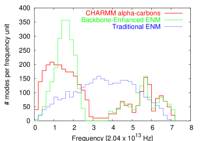
Figure 1: Density-of-states distribution for all-atom and elastic network models of trypsinogen. Frequency units are $({\rm Kcal}/{\rm mol}\,{\rm\AA}^{2}\,m_{p})^{1/2}=2.04\times 10^{13}\,{\rm Hz}$, where $m_{p}$ is the proton mass. Densities were estimated by counting the number of modes in bins of width 0.2, and normalizing the integral to 663, which is the total number of non-zero modes. The ENM (dotted blue) does not reproduce the bimodal distribution from the all-atom model (solid red); however, the BENM recovers the bimodal distribution (dashed green).

The best elastic network model of trypsinogen was obtained using a cutoff distance $r_{c}$ of approximately 7.75 Å, for which the optimal value of $\gamma$ is 53.4 Kcal/mol Ų, yielding a value of $D_{{\bf x}_{\alpha}}=312.9$ in a sharp minimum with respect to $r_{c}$. The density-of-states distribution for the elastic network model is unimodal, unlike that for the all-atom model (Fig. 1).

Although the ENM treats all alpha-carbon pairs equally, the distribution of distances between successive alpha-carbons along the protein backbone is known to be tightly centered about 3.8 Å. In addition, two of the six alpha-carbons nearest to a typical alpha-carbon are backbone neighbors, which might explain why 1/3 of the CHARMM-derived modes have significantly higher frequencies than the others. We therefore wondered whether the ENM might be improved by enhancing interactions between backbone neighbors.

Indeed, a more accurate coarse-grained model is obtained by using a force constant enhanced by a factor of $\epsilon$ for interactions between alpha-carbons that are neighbors on the backbone. Minimization of $D_{{\bf x}_{\alpha}}$ for such a backbone-enhanced elastic network model (BENM) with respect to $\epsilon$ and $r_{c}$ subject to Eq. (16) yields a model with $\epsilon=42$, $r_{c}=10.5$ Å, and $\gamma=4.26$ Kcal/mol Ų, resulting in a much lower value $D_{{\bf x}_{\alpha}}=102.3$. The density-of-states distribution for this model agrees quite well with that of the all-atom model (Fig. 1), especially considering that the model is optimized with respect to $D_{{\bf x}_{\alpha}}$, which does not directly involve the density-of-states distribution. The agreement is especially good for the high-frequency modes, suggesting that a uniform force constant is a reasonable approximation for interactions between alpha-carbons that are backbone neighbors. Furthermore, the overlap $\sum_{i=1}^{N}\sum_{j=1}^{N}|{\bf v}_{i}^{(\gamma){\dagger}}\bar{\bf v}_{j}|^{2}/N$ for the 223 highest-frequency modes is 0.99, indicating that the spaces of the high-frequency eigenvectors are nearly identical between the BENM and all-atom models. In contrast, the low-frequency distribution of BENM states is narrower than that of the all-atom model, indicating that a uniform force constant is a poorer approximation for interactions between alpha-carbons that are not backbone neighbors.

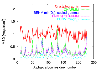
Figure 2: Mean-squared displacements of alpha-carbon positions for trypsinogen residues 10–229 obtained from normal-modes simulations using CHARMM (dashed green), a BENM with parameters that minimize $D_{{\bf x}_{\alpha}}$ with respect to CHARMM (dotted blue), the same BENM but with $\gamma$ adjusted to better agree with CHARMM MSDs (fine-dotted magenta), and an ENM with parameters adjusted to agree with CHARMM MSDs (dash-dotted cyan). Values were calculated at $T=300$ K using the Equipartition Theorem. Harmonic vibrations at thermal equilibrium are known to inadequately model crystallographic MSDs, which include other sources of disorder (solid red) Go et al. (1983).

Both the BENM and the ENM yield patterns of alpha-carbon MSDs that are similar to that of the all-atom model (Fig. 2). Because there are fewer low-frequency BENM modes than low-frequency CHARMM modes (Fig. 1), the BENM MSDs are consistently smaller than the CHARMM MSDs; however, the BENM MSDs may be improved by selecting $\gamma=1.2$ Kcal/mol Ų (Fig. 2). These improved MSDs come at the cost of a higher value of $D_{{\bf x}_{\alpha}}=528.4$, and a change in the frequency scale by a factor $(1.2/4.3)^{1/2}=0.53$, resulting in a poor model of the density-of-states distribution. The ENM with parameters that minimize $D_{{\bf x}_{\alpha}}$ exhibits poor MSDs (not shown); however, an ENM with $r_{c}=15.4$ Å and $\gamma=0.4$ Kcal/mol Ų yields MSDs that agree well with those of the CHARMM model (Fig. 2). In agreement with previous results using the ENM Atilgan et al. (2001), we confirmed that the parameters of both the ENM and BENM may be adjusted to yield a reasonable model of crystallographic MSDs (not shown).

Next consider the problem of quantifying allosteric effects in proteins Ming and Wall (2005). In allosteric regulation, molecular interactions cause changes in protein activity through changes in protein conformation. Although the importance of considering continuous conformational distributions in understanding allosteric effects was recognized by Weber Weber (1972), theories of allosteric regulation that consider continuous conformational distributions have been lacking. We began to develop such a theory by defining the allosteric potential as the Kullback-Leibler divergence $\bar{D}_{\bf x}$ between protein conformational distributions before and after ligand binding, and by calculating changes in the conformational distribution of the full protein-ligand complex in the harmonic approximation Ming and Wall (2005). Here we use the expression for the marginal distribution in Eq. (13) to calculate an equation for the allosteric potential in the harmonic approximation, and apply it to analyze allosteric mechanisms in trypsinogen.

Let ${\bf x}_{p}$ be the protein coordinates selected from the coordinates ${\bf x}$ of a protein-ligand complex. $P^{\prime}({\bf x}_{p})$ and $P({\bf x}_{p})$ are the protein conformational distributions with and without a ligand interaction. Eq. (13) enables $P^{\prime}({\bf x}_{p})$ to be calculated from the full conformational distribution $P^{\prime}({\bf x})$ of the protein-ligand complex. The equation for the allosteric potential in the harmonic approximation follows from the theory developed in ref. Ming and Wall (2005):

$$\bar{D}_{{\bf x}}=\sum_{i=1}^{3N_{p}}\left(\ln{\bar{\omega}^{\prime}_{i}\over{\omega}_{i}}+{1\over{2k_{B}T}}{\omega}_{i}^{2}\left|{\bf{v}}^{\dagger}_{i}\Delta{\bf x}_{p,{0}}\right|^{2}+{1\over 2}\sum_{j=1}^{3N_{p}}{{\omega}_{j}^{2}\over{\bar{\omega}^{\prime 2}_{i}}}\left|{{\bf\bar{v}}^{\prime{\dagger}}_{i}}{\bf{v}}_{j}\right|^{2}-{1\over 2}\right).$$ (17)

In Eq. (17), $\bar{\omega}^{\prime 2}$ and ${\bf\bar{v}}^{\prime}_{i}$ are the $i^{\rm th}$ eigenvalue and eigenvector of the matrix ${\bf\bar{H}}$ calculated for the protein atoms of the protein-ligand complex, $\omega_{i}^{2}$ and ${\bf v}_{i}$ are the eigenvalue and eigenvector of mode $i$ of the apo-protein, and $\Delta{\bf x}_{p,0}={\bf x}^{\prime}_{p,0}-{\bf x}_{p,0}$ is the difference between the equilibrium coordinates of the protein with and without the ligand interaction. The term $\sum_{i=1}^{3N_{p}}\ln{\bar{\omega}^{\prime}_{i}/\omega_{i}}$ is proportional to the change in configurational entropy of the protein releasing the ligand, and the term $\sum_{i=1}^{3N_{p}}{\omega}_{i}^{2}\left|{\bf{v}}^{\dagger}_{i}\Delta{\bf x}_{p,{0}}\right|^{2}/2k_{B}T$ is proportional to the potential energy required to deform the apo-protein into its equilibrium conformation in the protein-ligand complex.

We used Eq. (17) to calculate changes in the configurational distribution of local regions of trypsinogen upon binding bovine pancreatic trypsinogen inhibitor (BPTI). BPTI binds in the active site and exerts an allosteric effect, enhancing the affinity of trypsinogen for Val-Val Bode (1979). Alpha-carbon coordinates for 223 residues were obtained from a crystal structure of trypsinogen in complex with BPTI (residues 7–229 from PDB entry 4TPI Bode et al. (1984), including theoretically modeled residues 7–9), and were used directly to construct backbone-enhanced elastic network models of apo-trypsinogen and the trypsinogen-BPTI complex. As suggested by the refined trypsinogen model above, both models used $r_{c}=10.5$ Å, $\gamma=4.26$ Kcal/mol Ų, and $\epsilon=42$.

Local changes in the conformational distribution of trypsinogen were analyzed by considering changes in the neighborhood of each alpha-carbon atom. A neighborhood was defined by selecting the atom of interest plus its five nearest neighbors, and the matrix ${\bf\bar{H}}$ was calculated for these six atoms in the models both with (yielding ${\bf\bar{H}}^{\prime}$) and without (yielding ${\bf\bar{H}}$) the BPTI interaction. A local value of $\bar{D}_{\bf x}$ was obtained using the eigenvalues and eigenvectors of ${\bf\bar{H}}^{\prime}$ and ${\bf\bar{H}}$ in a suitably modified version of Eq. (17).

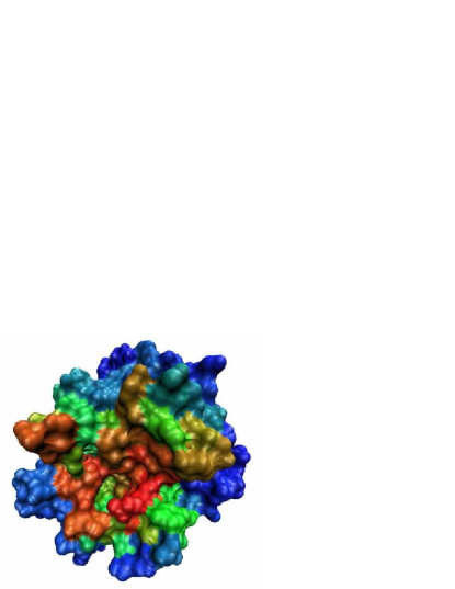
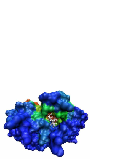
Figure 3: Visualization of local sites on the surface of trypsinogen that exhibit a large change in the conformational distribution upon binding BPTI. Values of $\bar{D}_{\bf x}$ are mapped to a logarithmic temperature scale, with red coloring indicating large values. Changes are large both in the BPTI-binding site (left) and in the Val-Val binding site (right). There is a $90^{\circ}$ rotation about the x-axis between the left and right panels.

Not surprisingly, we found that the local values of $\bar{D}_{\bf x}$ were relatively large in the neighborhood of the BPTI-binding site (Fig. 3, left panel). Values of $\bar{D}_{\bf x}$ elsewhere on the surface were smaller, with one interesting exception: values in the Val-Val binding site were comparable to those in the BPTI-binding site (Fig. 3, right panel).

We also calculated local values of $\bar{D}_{\bf x}$ for the Val-Val interaction, which causes the crystal structure of trypsinogen to resemble that of active trypsin Bode et al. (1978, 1984). We found that values were relatively large in the neighborhood of Ser 195, which is the key catalytic residue for trypsin and other serine proteases: the value of $\bar{D}_{\bf x}$ in this neighborhood was 40^th highest of 223 residues in the crystal structure; 11^th of all residues not directly interacting with the Val-Val in the model; the highest of all residues located at least as far as Ser 195 is from the Val-Val ligand; and greater than that for 20 of 60 residues located closer to the ligand. Calculations for both the BPTI interaction and the Val-Val interaction therefore indicate that there is a relatively strong communication between the regulatory and active sites of trypsinogen.

Considering models beyond the ENM and BENM (and even models beyond proteins), the theory presented here leads to a general prescription for modeling harmonic vibrations using coarse-grained models of materials. To optimally model the all-atom conformational distribution, always use an energy scale for interactions that eliminates the discrepancy due to differences in the eigenvectors (Eq. (16)), and select the coarse-grained model for which the entropy of the conformational distribution is the largest (first term of Eq. (15)).

Although traditional elastic network models can explain characteristics of the functions and dynamics of proteins Yang et al. (2005), the present study shows that they provide a poor approximation to the conformational distribution calculated from all-atom models of harmonic vibrations of proteins. Model accuracy is significantly improved by using a backbone-enhanced elastic network model, which strengthens interactions between atoms that are nearby in terms of covalent linkage. Although the backbone-enhanced model appears to accurately capture the high-frequency alpha-carbon vibrations of an all-atom model, the model less accurately captures the slower, large-scale harmonic vibrations (which in turn are known to poorly approximate the full spectrum of highly nonlinear, large-scale protein motions).

We also find that the allosteric potential is a useful tool for computational analysis of allosteric mechanisms in proteins. Using calculations of the allosteric potential, communication between the regulatory and active sites of trypsinogen was observed in a purely mechanical, coarse-grained model of protein harmonic vibrations that does not consider mean conformational changes or amino-acid identities, supporting prior arguments for the possibility of allostery without a mean conformational change Cooper and Dryden (1984). It will be interesting to perform similar analyses on a wide range of all-atom and coarse-grained models of protein vibrations, and to use more realistic calculations of free-energy landscapes Garcia and Sanbonmatsu (2001) to more accurately model changes in protein conformational distributions.

This work was supported by the US Department of Energy.

References

- Frauenfelder and Wolynes (1985) H. Frauenfelder and P. G. Wolynes, Science 229, 337 (1985).
- Kullback and Leibler (1951) S. Kullback and R. Leibler, Annals of Math. Stats. 22, 79 (1951).
- Ming and Wall (2005) D. Ming and M. E. Wall, Proteins 59, 697 (2005).
- Atilgan et al. (2001) A. R. Atilgan, S. R. Durell, R. L. Jernigan, M. C. Demirel, O. Keskin, and I. Bahar, Biophys. J. 80, 505 (2001).
- Brooks et al. (1983) B. Brooks, R. Bruccoleri, B. Olafson, D. States, S. Swaminathan, and M. Karplus, J. Comput. Chem. 4, 187 (1983).
- Zheng and Brooks (2005) W. Zheng and B. Brooks, Biophys. J. 89, 167 (2005).
- Tirion (1996) M. M. Tirion, Phys. Rev. Lett. 77, 1905 (1996).
- Bode et al. (1984) W. Bode, J. Walter, R. Huber, H. R. Wenzel, and H. Tschesche, Eur. J. Biochem. 144, 185 (1984).
- Go et al. (1983) N. Go, T. Noguti, and T. Nishikawa, Proc. Natl. Acad. Sci. USA 80, 3696 (1983).
- Weber (1972) G. Weber, Biochemistry 11, 864 (1972).
- Bode (1979) W. Bode, J. Mol. Biol. 127, 357 (1979).
- Bode et al. (1978) W. Bode, P. Schwager, and R. Huber, J. Mol. Biol. 118, 99 (1978).
- Yang et al. (2005) L. W. Yang, X. Liu, C. J. Jursa, M. Holliman, A. J. Rader, H. A. Karimi, and I. Bahar, Bioinformatics 21, 2978 (2005).
- Cooper and Dryden (1984) A. Cooper and D. T. Dryden, Eur. Biophys. J. 11, 103 (1984).
- Garcia and Sanbonmatsu (2001) A. E. Garcia and K. Y. Sanbonmatsu, Proteins 42, 345 (2001).