Alternative mechanisms of structuring biomembranes: Self-assembly vs. self-organization

Abstract

We study two mechanisms for the formation of protein patterns near membranes of living cells by mathematical modelling. Self-assembly of protein domains by electrostatic lipid-protein interactions is contrasted with self-organization due to a nonequilibrium biochemical reaction cycle of proteins near the membrane. While both processes lead eventually to quite similar patterns, their evolution occurs on very different length and time scales. Self-assembly produces periodic protein patterns on a spatial scale below 0.1 µm in a few seconds followed by extremely slow coarsening, whereas self-organization results in a pattern wavelength comparable to the typical cell size of 100 µm within a few minutes suggesting different biological functions for the two processes.

Living cells display internal structures on various lenght scales, that are regulated dynamically. Examples include the organisation of nerve cells into axon, body and dendrites Alberts or the occurrence of short-lived signaling patches in the membrane of chemotaxing amoebae Manahan:2004 . The origin of many of those structures is a nonuniform distribution of biochemical molecules, that can be achieved by a spontaneous symmetry breaking through local fluctuations. The diversity of time and length scales in cellular structures strongly suggest that a variety of mechanisms participate in the structuring process. From a physics perspective, one can distinguish at least two different classes of processes: self-assembly and self-organization Misteli:2001 .

Self-assembly implies spatial structuring as a result of minimization of the free energy in a closed system. Hence, a self-assembled structure corresponds to a thermodynamic equilibrium. A prominent example for self-assembly in single cells is phase separation of lipids and proteins due to macromolecular interactions. Phase separation occurs if the interaction energies dominate the entropy contribution. Model membranes show a phase separation due to lipid-lipid interactions Veatch:2002 ; McConnell:2003 or lipid-protein interactions Glaser:1996 (for a critical discussion see also Murray:1999 ). Theoretical analysis of phase separation in biomembranes has been mainly restricted to free energy considerations May:2002 ; Anderson:2000 , which can predict the final equilibrium state, but do not capture the transient dynamics.

Self-organization, in contrast, requires a situation far away from thermodynamic equilibrium and is possible only in open systems with an external energy source. One prominent example is pattern formation in reaction-diffusion systems, which has first been proposed by Turing Turing:1952 and later on become influential in development biology Gierer:1972 . The key ingredients are nonlinear self-enhancing reactions, a supply of chemical energy and competing diffusion of the involved molecules. Experimental patterns in single cells that are successfully modelled by reaction-diffusion equations include calcium waves Falcke:2004 and protein distributions in E. coli Howard:2005 .

In the vicinity of membranes molecular interactions and reaction-diffusion processes occur simultaneously. In this Letter we discuss and compare two dynamical models for the alternative mechanisms of pattern formation near the cell membrane: model I describes self-assembly of protein domains due to lipid-protein interactions and model II describes an active reaction-diffusion mechanism resulting in self-organization of proteins.

The two models are based on the properties of the GMC proteins reviewed in Blackshear:1993 ; McLaughlin:2002 , which play a critical role in the development of the neural system Frey:2000 and in the regulation of cortical actin-based structures and cell motility Laux:2000 . A key result is that both models display similar qualitative dynamical behavior but act on largely different time and length scales. Model I leads to the formation of stationary domains on a submicrometer scale within seconds. A slow coarsening process follows the expected power law. Phase separation arises from a relaxational process into thermodynamic equilibrium, where the equilibrium state is characterized by vanishing fluxes. Model II leads to the formation of large stationary structures on the scale of a eukaryotic cell within 10 min. The steady state of this active phase separation (= phase separation from self-organization) is characterized by nonzero fluxes.

Model I is based on attractive interactions of GMC proteins with acidic lipids in membranes AWWH00 . In this mechanism (Fig. 1 (a)) proteins (area fraction $c_{m}$) are associated with a lipid membrane, consisting of type 1 (area fraction $c_{l}$) and type 2 (area fraction $1-c_{l}$) lipids of identical size. The size ratio between proteins and lipids is $N$. Proteins interact attractively with type 1 lipids. Proteins and lipids are allowed to diffuse in the plane of the membrane. The number of bound proteins and the average membrane composition are conserved quantities. We write the free energy of the protein covered membrane similar to May:2002 as

$$F=k_{B}TN_{a}\int\,dA\Bigg{[}f_{l}+\frac{\chi}{2}\left(\nabla{}c_{l}\right)^{2}\Bigg{]}$$ (1)

where $dA$ denotes integration over the membrane surface, $N_{a}$ denotes the number of lipids per unit area and

$$f_{l} = c_{l}\ln{}c_{l}+(1-c_{l})\ln{}(1-c_{l})+$$ (2)

$$\frac{c_{m}}{N}\ln{}c_{m}+\frac{1-c_{m}}{N}\ln{}(1-c_{m})-uc_{l}c_{m}\,.$$

The local part of the free energy (2) consists of the entropic contributions of the lipid (first and second term) and the protein phase (third and fourth term) and the interaction energy between lipids and proteins (last term) par:u . For simplicity we assume that electrostatic repulsion and non-electrostatic attraction in the lipid and protein phase cancel locally. This is somewhat arbitrary, but does not change the nature of the results as long as demixing is governed by lipid-protein interactions. The non-local part of the free energy (1) is governed by the interfacial energy in the lipid phase, which is a small quantity. For the parameter $\chi$ we set $\chi\approx{}\frac{1}{2}u_{l}l^{2}$ from Cahn-Hilliard Theory Cahn:1958 where $u_{l}$ and $l$ are the typical interaction energy (on the order of several $k_{\rm B}T$) and length (on the order of a lipid headgroup size, i.e. $l\approx{}1-2$ nm), respectively. Evolution equations for $c_{l}$ and $c_{m}$ are obtained using linear nonequilibrium thermodynamics and the mass balance equations to give

$$\begin{array}[]{lclclcl}\partial_{t}c_{l}&=&-\nabla\cdot\vec{j}_{l}&\quad\mbox{with}&\vec{j}_{l}&=&-M_{l}\nabla\frac{\delta{}F}{\delta{}c_{l}}\\ \partial_{t}c_{m}&=&-\nabla\cdot\vec{j}_{m}&\quad\mbox{with}&\vec{j}_{m}&=&-M_{m}\nabla\frac{\delta{}F}{\delta{}c_{m}}\,.\end{array}$$ (5)

More specifically, the fluxes $\vec{j}_{l}$ and $\vec{j}_{m}$ are given by

$$\vec{j}_{l} = -D_{l}\left[\nabla c_{l}-c_{l}(1-c_{l})\left(u\nabla c_{m}+\chi\nabla^{3}c_{l}\right)\right]$$ (6)

$$\vec{j}_{m} = -D_{m}\left[\nabla c_{m}-Nc_{m}(1-c_{m})u\nabla c_{l}\right]\,,$$ (7)

where $D_{l}=M_{l}k_{B}TN_{a}$ and $D_{m}=M_{m}k_{B}TN_{a}$.

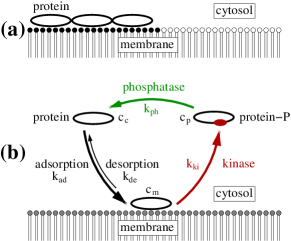
Figure 1: Schematic depiction of models I (a) and II (b). (a) The membrane consists of a mixture of type 1 (black) and 2 (white) lipids with adsorbed proteins. (b) Proteins undergo a cycle of phosphorylation and dephosphoylation as explained in the text.

.

Model II is based on a biochemical cycle of GMC phosphorylation and dephosphorylation, called myristoyl-electrostatic (ME) switch Thelen:1991 . In contrast to model I, we will assume that all different lipid species are distributed uniformely in the membrane. In this phase separation model (Fig. 1 (b)) a protein can associate reversibly with the membrane following a mass action law. On the membrane proteins are irreversibly phosphorylated by a protein kinase, which disrupts membrane binding immediately and translocates the protein into the cytosol where it is dephosphorylated by a phosphatase. We can cast these processes into a three-variable reaction-diffusion model of the following form

$$\partial_{t}c_{m} = k_{ad}(1-c_{m})c_{c}-k_{de}c_{m}-$$ (8)

$$k_{ki}(1-c_{m})\frac{c_{m}}{k_{m}+c_{m}}+D_{m}\nabla^{2}c_{m}$$

$$\partial_{t}c_{c} = k_{de}c_{m}-k_{ad}(1-c_{m})c_{c}+k_{ph}c_{p}+D_{c}\nabla^{2}c_{c}$$ (9)

$$\partial_{t}c_{p} = k_{ki}(1-c_{m})\frac{c_{m}}{k_{m}+c_{m}}-k_{ph}c_{p}+D_{c}\nabla^{2}c_{p}\,.$$ (10)

$c_{m}$, $c_{c}$ and $c_{p}$ denote the concentrations of membrane bound, cytosolic unphosphorylated and cytosolic phosphorylated proteins, respectively. $k_{ad}$ and $k_{de}$ denote the rate constants of membrane association and dissociation of the unphosphorylated protein and $k_{ki}$ and $k_{ph}$ denote the enzymatic activities of the kinase and phosphatase. For the kinase activity we have used a Michaelis-Menten type kinetics Verghese:1994 , whereas we have neglected this property for the phosphatase, assuming that the concentration of phosphorylated proteins is well below the respective Michaelis-Menten constant Seki:1995 . Based on the properties of protein kinase C we assume, that the kinase needs lipids for full activation Cockcroft:2000 ; Bell:1991 and that membrane bound proteins decrease the available membrane space and thus the kinase activity Glaser:1996 . Eqs. (8)–(10) constitute a non-equilibrium system, since the kinase activity is sustained and consumes ATP which is produced by the metabolism. The total protein concentration $c_{t}=\frac{1}{V}\int{}dV\,(c_{m}+c_{p}+c_{c})$ is conserved.

The parameters for both models have been taken from experiments. First we consider the linear stability of the uniform steady states (Fig. 2). In both models we can identify a region of linear instability, characterized by real positive eigenvalues. Using the Maxwell construction and tie-lines we calculated for model I the equilibrium state for a given uniform state and identified a metastable region, where a stable uniform state coexists with a stable demixed state. The demixed state is characterized by a phase with a high concentration in protein and lipid 1 and a phase with a low concentration in protein and lipid 1. Using continuation methods we computed stationary solutions for model II. Fixing the wavelength to 120 µm (comparable to the size of a eukaryotic cell) one can also identify regions, where a linearly stable uniform solution coexists with a linearly stable stationary periodic solution.

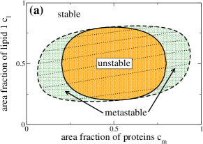
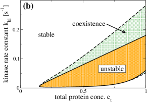
Figure 2: (a) Phase diagrams with tie-lines for the phase separation in model I and (b) phase diagram for the active phase separation in model II. Parameters in (a) are $N=25$ and $u=1.0$ and in (b) are $N=25$, $D_{m}=0.04\,\mu$m² s^-1 Swaminathan:1997 ; Seksek:1997 , $D_{c}=20\,\mu$m² s^-1, $k_{ad}=1$ s^-1 Arbuzova:1997 , $k_{de}=0.005$ s^-1 Arbuzova:1997 , $k_{m}=0.01$ Verghese:1994 , $k_{ph}=0.2$ s^-1 Thelen:1991 .

.

Figs. 3 (a) and (b) show the largest eigenvalues for both models from the linearly unstable regions in Figs. 2 (a) and (b). The instabilities belong to the type II_s class Cross:1993 , which is characterized by a real critical eigenvalue with wave number zero and can be attributed to the conservation relations in both models. Although both models have instabilities of the same type they develop on very different length and time scales. The wavelength of the fastest growing mode $\lambda_{m}$ in model I is linked to the molecular interaction length. In our example in Fig. 3 a it is on the scale of 50 nm with a growth rate of 10 s^-1. In contrast, $\lambda_{m}$ of model II is determined by kinetic rate and diffusion constants and is of the order of 10 µm. In the example in Fig. 3 b the corresponding growth rate is 0.01 s^-1.

Figure 3: Dispersion relations for models I (a) and II (b) for the uniform solution. Shown is only the largest (real) eigenvalue. Parameters in (a) are $N=25$, $c_{l}=0.2$, $c_{m}=0.5$, $u=1.01$, $D_{l}=1.0\,\mu$m² s^-1 Kusba:2002 , $D_{m}=0.04\,\mu$m² s^-1, $\chi=10^{-6}\,\mu$m² and in (b) $c_{t}=0.5$, $k_{ki}=0.05$ s^-1. Remaining parameters are as in Fig. 2 (b).

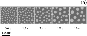
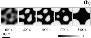
Figure 4: Snapshots of a two-dimensional numerical simulations of models I (a) and II (b) with periodic boundary conditions. Shown is the concentration of membrane bound protein $c_{m}$. Parameters in (a) and (b) are as in Fig. 3 (a) and (b), respectively.

The results of the linear stability were confirmed by numerical simulations in two dimensions with periodic boundary conditions. Simulations were started from the uniform steady state with small amplitude perturbations. Figs. 4 (a) and 4 (b) show exemplary two simulations for models I and II with parameter values from the linearly unstable regions in Fig 2. In both models stationary structures develop, which are not stable but display a coarsening behavior for later stages.

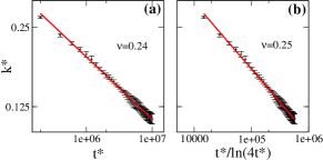
Figure 5: Late stage behavior of model I ($t^{\ast}=tD_{l}/\chi$, $k^{\ast}=k\sqrt{\chi}$). Shown are loglog-plots of the evolution of the mean wave number of the structure factor of the membrane bound protein concentration with time (a) or a modified time (b) as described in the text. The exponent $\nu$ of the power law was obtained by a least square fit. Parameters are the same as in Fig. 3 (a).

.

For model I we found the scaling law $\bar{k}(t)=at^{-\nu}$ (Fig. 5) with an exponent $\nu\approx{}1/4$ consistent with a modified Lifshitz-Slyosov-Wagner theory Bray:1995 for concentration dependent mobility coefficients. Since we are considering the two-dimensional case one should rather expect a growth law $\bar{k}(\tau)=a\tau^{-\nu}$ with a modified time scale $\tau=t/\ln(4t)$ Rogers:1989 . However, on the time scale of our numerical experiments both growth laws yielded similar exponents. Although the initial growth is very fast the initally observed wave numbers are small. To obtain structures on the scale of the cell coarsening has to occur over several orders of magnitude with $\nu=1/4$, which is a slow process. The possible scaling behavior of model II is irrelevant for practical purposes since the initially developed structures are already on a scale comparable to the system size and the first or second coarsening step will lead to polarized cells with a single domain of high concentration of membrane bound proteins. One can easily see in Fig. 4 (b) that large structures have appeared after ten minutes and within one hour coarsening is complete.

In this Letter we have introduced and analyzed two alternative models for pattern formation of GMC proteins. GMC proteins are on the one hand found to form domains by virtue of their attractive electrostatic interaction with acidic lipids from self-assembly. On the other hand, they can exploit an ATP-driven phosphorylation-dephosphorylation cycle (myristoyl-electrostatic switch) for their self-organization. The striking difference between both mechanisms lies in the relevant time and length scales. The spinodal length scale of the phase separation in model I is closely linked to the molecular interaction length in the lipid phase. For fluid membranes under physiological conditions the relevant interaction scale is comparable to the size of a lipid molecule ($\approx 1\,$nm). The initial structure formation is fast with growth rates of the order of 10 s^-1, but the coarsening process follows a scaling law. Thus coarsening does not lead to structures on the size of the cell in a biologically relevant time. The reaction-diffusion mechanism (model II) leads initially to large structures, which are on the scale of an eukaryotic cell. A rough estimate for the length scale is given by the quantity $\sqrt{D\tau}$, where $D\approx{}$10 µm² s^-1 is the typical intracellular diffusion constant of a protein and $\tau=10\,$s is a typical time for a biochemical reaction. This yields a length scale of $\approx{}$10 µm. A combination of both mechanism leads to a more complicated model, that displays oscillatory dynamics and traveling domains John:2005 . Here, we have used specific physical and chemical properties of GMC proteins, but the typical scales for molecular interaction energies and ranges as well as for reaction rates and diffusion constants will be comparable for other processes near membranes. We propose that both mechanisms are relevant for different aspects of structuring membranes: protein-lipid interactions are suitable for rapid structuring of membranes on a submicrometer scale, whereas reaction and diffusion of proteins produce a structure on the scale of the size of typical eukaryotic cell within minutes and are potentially useful for polarizing a whole cell into two main compartments (e. g. front and back).

References

- (1) B. Alberts et al., Molecular Biology of the Cell (Garland Publishing, 1994).
- (2) C. L. Manahan et al., Annu. Rev. Cell Dev. Biol. 20, 223 (2004).
- (3) T. Misteli, J. Cell Biol. 155, 181 (2001).
- (4) S. L. Veatch and S. L. Keller, Phys. Rev. Lett. 89, 268101 (2002).
- (5) H. M. McConnell and M. Vrljic, Annu. Rev. Biophys. Biomol. Struct. 32, 469 (2003).
- (6) M. Glaser et al., et al., J. Biol. Chem. 271, 26187 (1996).
- (7) D. Murray et al., Biophys. J. 77, 3176 (1999).
- (8) S. May, D. Harries, and A. Ben-Shaul, Phys. Rev. Lett. 89, 268102 (2002).
- (9) T. G. Anderson and H. M. McConnell, J. Phys. Chem. 104, 9918 (2000).
- (10) A. Turing, Philos. Trans. R. Soc. London, ser. B 237, 37 (1952).
- (11) A. Gierer and H. Meinhardt, Kybernetik 12, 30 (1972).
- (12) M. Falcke, Adv. Phys. 53, 255 (2004).
- (13) M. Howard and K. Kruse, J. Cell Biol 168, 533 (2005).
- (14) P. J. Blackshear, J. Biol. Chem. 268, 1501 (1993).
- (15) S. McLaughlin et al., Ann. Rev. Biophys. Biomol. Struct. 31, 151 (2002).
- (16) D. Frey et al., J. Cell Biol. 149, 1443 (2000).
- (17) T. Laux et al., J. Cell Biol. 149, 1455 (2000).
- (18) A. Arbuzova et al., Biochemistry 39, 10330 (2000).
- (19) The contribution of the protein-lipid interactions to the electrostatic energy of the membrane is , with nm, (charge of proteins), (charge of type 1 lipids), nm2 (area of lipid headgroup), and .
- (20) J. Cahn and J. Hilliard, J. Chem. Phys. 28, 258 (1958).
- (21) M. Thelen et al., Nature 351, 320 (1991).
- (22) G. M. Verghese et al., J. Biol. Chem. 269, 9361 (1994).
- (23) K. Seki, H.-C. Chen, and K.-P. Huang, Arch. Biochem. Biophys. 316, 673 (1995).
- (24) S. Cockcroft, ed., Biology of Phosphoinositides (Oxford University Press, 2000), and references therein.
- (25) R. M. Bell and D. J. Burns, J. Biol. Chem. 266, 4661 (1991).
- (26) R. Swaminathan, C. P. Hoang, and A. S. Verkmann, Biophys. J. 72, 19000 (1997).
- (27) O. Seksek, J. Biwersi, and A. S. Verkman, J. Cell Biol. 138, 131 (1997).
- (28) A. Arbuzova et al., J. Biol. Chem. 272, 27167 (1997).
- (29) M. C. Cross and P. C. Hohenberg, Rev. Mod. Phys. 65, 851 (1993).
- (30) J. Kusba et al., Biophys. J. 82, 1358 (2002).
- (31) A. J. Bray and C. L. Emmott, Phys. Rev. B 52, R685 (1995).
- (32) T. M. Rogers and R. C. Desai, Phys. Rev. B 39, 11956 (1989).
- (33) K. John and M. Bär, Phys. Biol. 2, 123 (2005).