General theory and mathematical aspects Computer simulation Fluctuation phenomena, random processes, noise, and Brownian motion

Dynamic model for failures in biological systems

Abstract

A dynamic model for failures in biological organisms is proposed and studied both analytically and numerically. Each cell in the organism becomes dead under sufficiently strong stress, and is then allowed to be healed with some probability. It is found that unlike the case of no healing, the organism in general does not completely break down even in the presence of noise. Revealed is the characteristic time evolution that the system tends to resist the stress longer than the system without healing, followed by sudden breakdown with some fraction of cells surviving. When the noise is weak, the critical stress beyond which the system breaks down increases rapidly as the healing parameter is raised from zero, indicative of the importance of healing in biological systems.

Many systems in nature under steady external driving are led into failures. Examples are diverse ranging from disordered heterogeneous materials, earthquakes, and even to social processes. The fiber bundle models, describing well these systems, have received considerable attention [1]. Most studies of fiber bundles are based on the recursive breaking dynamics at discrete time step. One of the typical features in the models is that local stress arising from external driving tends to produce avalanches of microscopic failures, resulting in stationary macroscopic breakdown of the system. The main issue here is thus the life time of a fiber bundle and the avalanche size distribution under various conditions [2, 3, 4]. There are shortcomings, however, in discrete dynamics: It cannot describe the time evolution in real continuous time, for which a remedy has been suggested recently [5].

Failures are also observed in biological systems, as a consequence of disease for instance; these are different from other failures in the sense that there may exist healing, in reparative or regenerative ways. Here the evolution to the stationary state appears more important than the stationary state itself.

In this Letter we extend our previous work on the dynamic model for failures in fiber bundles [5] to biological systems consisting of cells. Incorporating the effects of healing into the model in a manner similar to that used for neural networks [6], we derive equations of motion for biological organisms in the form of delay-differential equations. From this formulation, we obtain the evolution equation for the average number of living cells and find that there generally remains a finite fraction of living cells in the stationary state, manifesting the healing effects. This persists in the presence of noise, in sharp contrast to the case of no healing. The system is then explored numerically, which shows that the presence of healing assists the system to resist the stress longer before abrupt breakdown into the stationary state as well as increases the critical stress of external load that brings about the breakdown. The resulting behavior is reminiscent of the time course of degenerative disease progression such as diabetes, Alzheimer’s disease, and possibly AIDS. We thus believe our approach may serve as a prototype model for disease progression at the cellular level, for which only a phenomenological description is available so far [7].

We consider an organism consisting of $N$ cells under external stress characterized by load $F$. Each cell has its own tolerance and endures the stress below the tolerance, thus remaining alive. The cell may become dead, however, if the tolerance is exceeded. We assign “spin” variables to these in such a way that $s_{i}=-1\,(+1)$ for the $i$th cell alive (dead). The state of the organism is then described by the configuration of all the cells, $\mathbf{s}\equiv(s_{1},s_{2},...,s_{N})$. The total number $N_{-}$ of living cells is related with the average spin $\bar{s}\equiv N^{-1}\sum_{j}s_{j}$ via

$$N_{-}=\sum_{j=1}^{N}\frac{1-s_{j}}{2}=\frac{N}{2}(1-\bar{s}),$$ (1)

and we are interested in how $N_{-}$ evolves in time as well as its stationary value. The total stress on the $i$th cell can then be written in the form

$$\eta_{i}=f+\sum_{j}V_{ij}\,\frac{1+s_{j}}{2},$$ (2)

where $f=F/N$ is the stress directly due to the external load and $V_{ij}$ represents the stress transferred from the $j$th cell (in case that it is dead). The death of the $i$th cell with tolerance $h_{i}$ is determined according to:

$$\eta_{i}<h_{i}~{}\Rightarrow~{}s_{i}=-1$$

$$\ \eta_{i}>h_{i}~{}\Rightarrow~{}s_{i}=+1,$$

which, in terms of the local field $E_{i}\equiv(\eta_{i}-h_{i})(1-\bar{s})/2$, can be simplified as $s_{i}E_{i}>0$. This determines the stationary configuration at which the system eventually arrives.

For a more realistic description of the time evolution, we also take into consideration the uncertainty (“noise”) present in real situations, which may arise from imperfections, random variations, and other environmental influences. We thus begin with the conditional probability that the $i$th cell is dead at time $t{+}\delta t$, given that it is alive at time $t$. For sufficiently small $\delta t$, we may write [6]

$$p(s_{i}{=}+1,t{+}\delta t|s_{i}{=}-1,t;\mathbf{s}^{\prime},t{-}t_{d})=\frac{\delta t}{2t_{r}}\left[1+\tanh\beta E^{\prime}_{i}\right],$$ (3)

where $\mathbf{s}^{\prime}\equiv(s^{\prime}_{1},s^{\prime}_{2},\ldots,s^{\prime}_{N})$ represents the configuration of the system at time $t{-}t_{d}$ and $E^{\prime}_{i}=(\eta_{i}-h_{i})(1-\bar{s^{\prime}})/2$ is the local field at time $t{-}t_{d}$. Note the two time scales $t_{d}$ and $t_{r}$ here: $t_{d}$ denotes the time delay during which the stress is redistributed among cells while the refractory period $t_{r}$ sets the relaxation time (or life time). The “temperature” $T\equiv\beta^{-1}$ measures the width of the tolerance region of the cells or the noise level: In the noiseless limit $(T=0)$ the factor $(1+\tanh\beta E^{\prime}_{i})/2$ in eq. (3) reduces to the step function $\theta(E^{\prime}_{i})$, yielding the stationary-state condition. We also assign the non-zero conditional probability of the $i$th cell being repaired (regenerated) given that it is dead at time $t$, according to

$$p(s_{i}{=}-1,t{+}\delta t|s_{i}{=}+1,t;\mathbf{s}^{\prime},t{-}t_{d})=\frac{\delta t}{t_{0}},$$ (4)

where $t_{0}$ is the time necessary for cell regeneration. Equations (3) and (4) can be combined to give a general expression for the conditional probability

$$p(-s_{i},t{+}\delta t|s_{i},t;\mathbf{s}^{\prime},t{-}t_{d})=w_{i}(s_{i};\mathbf{s}^{\prime},t{-}t_{d})\delta t$$ (5)

with the transition rate

$$w_{i}(s_{i};\mathbf{s}^{\prime},t{-}t_{d})=\frac{1}{2t_{r}}\left[\left(a+\frac{1}{2}\right)+\left(a-\frac{1}{2}\right)s_{i}+\frac{1-s_{i}}{2}\tanh\beta E^{\prime}_{i}\right],$$ (6)

where the healing parameter $a\equiv t_{r}/t_{0}$ measures the relative time scale of relaxation and regeneration of a cell. Here we point out that $t_{d}$, $t_{r}$, $t_{0}$, and accordingly $a$ may be complicated functions of system properties like the average spin $\bar{s}$ and others, which may be incorporated into the model. In this work we restrict ourselves to the simplest case of these parameters being fixed.

The behavior of the organism is then governed by the master equation, which describes the evolution of the joint probability $P(\mathbf{s},t;\mathbf{s}^{\prime},t{-}t_{d})$ that the system is in state $\mathbf{s}^{\prime}$ at time $t{-}t_{d}$ and in state $\mathbf{s}$ at time $t$. Following the procedures in Ref. [5], we rescale time $t$ in units of the delay time $t_{d}$ and write accordingly the transition rate $w_{i}(s_{i};\mathbf{s}^{\prime})\equiv t_{d}w_{i}(s_{i};\mathbf{s}^{\prime},t{-}t_{d})$, which yields, in the limit $\delta t\rightarrow 0$,

$$\frac{d}{dt}P(\mathbf{s},t;\mathbf{s}^{\prime},t{-}1)=-\sum_{i}[w_{i}(s_{i};\mathbf{s}^{\prime})P(\mathbf{s},t;\mathbf{s}^{\prime},t{-}1)-w_{i}(-s_{i};\mathbf{s}^{\prime})P(F_{i}\mathbf{s},t;\mathbf{s}^{\prime},t{-}1)]$$ (7)

with $F_{i}\mathbf{s}\equiv(s_{1},s_{2},...,-s_{i},s_{i+1},...,s_{N})$. Here it has been noted that contributions from the intermediate configurations $\mathbf{s}^{\prime}$ differing from $\mathbf{s}$ by only one cell survive; those from other configurations are of order $(\delta t)^{2}$ or higher and thus vanish in the limit $\delta t\rightarrow 0$. Then equations describing the time evolution of relevant physical quantities, with the average taken over $P(\mathbf{s},t;\mathbf{s}^{\prime},t{-}1)$, in general assume the form of differential-difference equations due to the delay in the stress redistribution. In particular, the average spin for the $k$th cell, $m_{k}(t)\equiv\langle s_{k}\rangle\equiv\sum_{\mathbf{s},\mathbf{s}^{\prime}}s_{k}P(\mathbf{s},t;\mathbf{s}^{\prime},t{-}1)$ satisfies

$$\tau\frac{d}{dt}m_{k}=\left(\frac{1}{2}-a\right)-\left(\frac{1}{2}+a\right)m_{k}+\left\langle\frac{\displaystyle{1-s_{k}}}{\displaystyle 2}\tanh\beta E^{\prime}_{k}\right\rangle$$ (8)

where $\tau\equiv t_{r}/t_{d}$ gives the relaxation time (in units of $t_{d}$).

To proceed further, we assume equal load sharing, i.e., that the stress is distributed to every cell uniformly. In this case we have $V_{ij}=\eta_{j}/N_{-}$ and accordingly, $(1-\bar{s})\eta_{i}=2f$ from eq. (2). The infinite-range nature of equal load-sharing allows one to replace $E^{\prime}_{k}$ by its average $\langle E^{\prime}_{k}\rangle=f-(h_{k}/2)[1-\bar{m}(t{-}1)]$, where it has been noted that $s^{\prime}$ is the configuration at time $t{-}1$, i.e., $\langle\bar{s}^{\prime}\rangle=N^{-1}\sum_{j}\langle\bar{s}^{\prime}_{j}\rangle=N^{-1}\sum_{j}m_{j}(t{-}1)\equiv\bar{m}(t{-}1)$. For convenience, we now rewrite eq. (8) in terms of the average number of living cells at time $t$. Defining $x_{k}\equiv(1-m_{k})/2$ and $\bar{x}\equiv N^{-1}\sum_{k}x_{k}=(1-\bar{m})/2$, we have, from eq. (1), $\langle N_{-}\rangle=N\bar{x}$ and thus obtain from eq. (8) the equation of motion for the average fraction of living cells:

$$\tau\frac{d}{dt}x_{k}(t)=a-\left(\frac{1}{2}+a\right)x_{k}(t)-\frac{1}{2}x_{k}(t)\tanh\beta[f{-}h_{k}\bar{x}(t{-}1)].$$ (9)

We first examine the stationary solution of eq. (9) with $dx_{k}/dt=0$:

$$x_{k}=\frac{2a}{(1+2a)+\tanh\beta(f{-}\bar{x}h_{k})},$$ (10)

which, upon averaging over the tolerance distribution $g(h)$, leads to the self-consistency equation for the average fraction of living cells or the “health status” of the organism

$$\bar{x}=\int dhg(h)\frac{2a}{(1+2a)+\tanh\beta(f-\bar{x}h)}.$$ (11)

It is obvious that regardless of noise, the complete breakdown, described by the null solution $\bar{x}=0$, is possible only for $a=0$, i.e., when cells are not regenerated or repaired. This contrasts with the case $a=0$, where noise usually gives rise to the breakdown of the system ($\bar{x}=0$) [5, 8]. It is thus concluded that the biological systems become robust against noise due to the cell regeneration effects.

In the noiseless limit ($T=0$) we replace the term $\tanh\beta(f{-}\bar{x}h)$ in eq. (11) by $\theta(f{-}\bar{x}h)-\theta(\bar{x}h{-}f)$, to obtain

$$\bar{x}=\int dhg(h)\left[\theta(h\bar{x}{-}f)+\frac{a}{1+a}\;\theta(f{-}h\bar{x})\right].$$ (12)

For a continuous distribution of the tolerance, we formally solve eq. (12) by simply performing the integration

$$\bar{x}=1-\frac{1}{1+a}\;G(f/\bar{x}),$$ (13)

where $G(h)=\int_{0}^{h}dh^{\prime}g(h^{\prime})$ is the cumulative distribution of the tolerance. Equation (13) shows that a majority of cells in general becomes dead at stress above a critical value $f_{c}$, which depends on $a$. This can be manifested with simple distributions, e.g., the bimodal distribution $g(h)=\rho\delta(h{-}f_{1})+(1-\rho)\delta(h{-}f_{2})$ with $0<f_{2}<f_{1}$. A simple integration leads to

$$\bar{x}=\left\{\begin{array}[]{ll}1&~{}\mbox{for}~{}f<f_{2}\bar{x}\\ (\rho+a)(1+a)^{-1}&~{}\mbox{for}~{}f_{2}\bar{x}<f<f_{1}\bar{x}\\ a(1+a)^{-1}&~{}\mbox{for}~{}f_{1}\bar{x}<f.\end{array}\right.$$

As $f$ is raised from zero in the system with $f_{2}<\rho f_{1}$, the first breakdown occurs at $f=f_{2}$, yielding $\bar{x}=(\rho+a)(1+a)^{-1}$, and subsequently the second one at $f=(\rho+a)(1+a)^{-1}f_{1}$. For $f_{2}>\rho f_{1}$, on the other hand, there appears only one breakdown at $f=f_{2}$. In these two cases the critical stress $f_{c}$, beyond which the system breaks down significantly, is thus given by $(\rho+a)(1+a)^{-1}f_{1}$ and $f_{2}$, respectively. Note that the survival fraction $a(1+a)^{-1}$ is negligible for small healing parameter ($a\ll 1$).

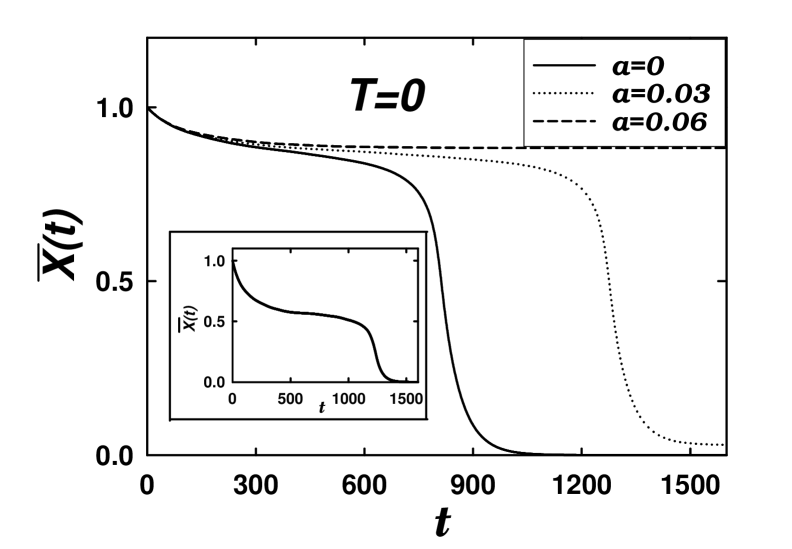
Figure 1: Evolution of the average fraction $\bar{x}$ of living cells with time $t$ (in units of the delay time) for the Gaussian distribution of $\bar{h}=1$ and $\sigma=0.2$ at $T=0$. The stress is $f=0.685$ slightly larger than $f_{c}(0)\approx 0.677$. Solid, dotted, and broken lines correspond to $a=0$, $0.03$, and $0.06$, respectively. Shown in the inset is the behavior for $\sigma=0.6$ (still at $T=0$ and $a=0$). The stress $f=0.522$ is again slightly larger than $f_{c}(0)\,(\approx 0.518$ for $\sigma=0.6$).

We now turn our attention to the time evolution of the system. We consider first the simplest case of equal load sharing, and integrate directly the equation of motion (9) in a numerical way. We consider the Gaussian distribution of the tolerance with unit mean and standard deviation $\sigma=0.2$, mostly in a system of $N=10^{4}$ cells. Other distributions including the Weibull distribution have also been considered, only to give essentially the same results. Specifically, we have used ten different configurations of the tolerance distribution and set the relaxation time $\tau=50$ and the time step $\Delta t=0.1$. These parameter values have been varied, only to give no appreciable difference except for the time scale.

We first display in fig. 1 the health status of the organism at $T=0$, with $f$ being slightly larger than the critical stress $f_{c}(a{=}0)\approx 0.677$. As reflected by the plateau, the system without healing resists the stress for some time before it breaks down completely. With small amount of healing, the duration of the plateau becomes longer and there remains a finite fraction of cells after the breakdown. We refer to this as the unhealthy state of the system [9]. Here further increase of $a$ makes the duration of the plateau extremely long and the system does not break down, implying that the healthy state of the organism persists. For $f$ is smaller than the critical stress $f_{c}(a{=}0)$, the average fraction $\bar{x}$ of living cells decreases very slowly (not shown) and the system remains healthy. Note also that the detailed degeneration behavior of the health status depends on the tolerance distribution. For example, a wider distribution in general brings about severer deterioration initially, followed by long duration of the unhealthy state before the breakdown (see the inset), similar to the progression of, e.g., AIDS.

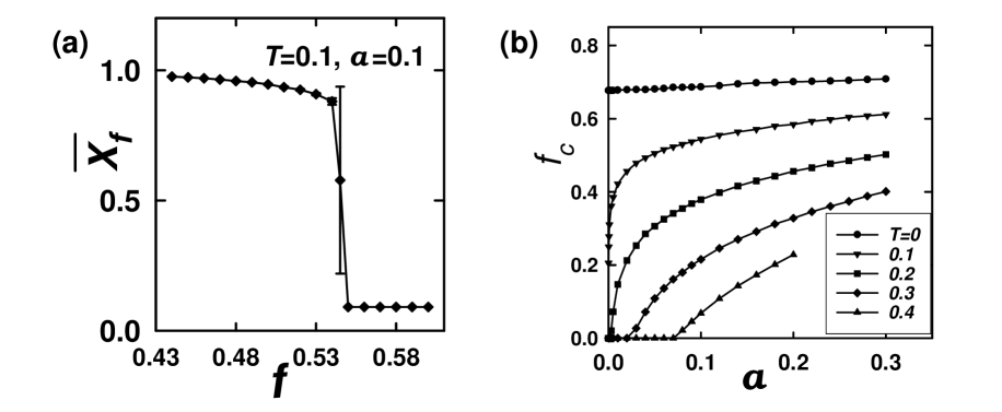
Figure 2: (a) Residual fraction $\bar{x}_{f}$ of living cells versus $f$ for $a=0.1$ at $T=0.1$. (b) Critical stress $f_{c}$ versus healing parameter $a$ at several temperatures.

More interesting results are obtained at finite noise levels. For $a=0$, non-negligible noise in the system eventually results in complete breakdown for any finite stress (i.e., $f_{c}=0$ at $T\gtrsim 0.1$ although there is numerical ambiguity at very low noise levels). When $a\neq 0$, on the other hand, the system may remain healthy up to some finite stress which depends on $a$, and thus $f_{c}$ does not vanish. To illustrate this, we plot in fig. 2(a) the residual fraction $\bar{x}$ as a function of $f$ for $a=0.1$ at $T=0.1$. It is clearly observed that the system becomes unhealthy abruptly near $f_{c}\approx 0.55$ as $f$ is increased. Figure 2(b) displays how the critical stress $f_{c}$ varies with the healing parameter $a$ at several noise levels. At $T=0$, $f_{c}$ is observed to increase very slowly with $a$. In sharp contrast, at low but finite noise levels ($T\ll 1$), which are presumably the case for biological systems in nature, $f_{c}$ increases very rapidly as $a$ is raised from zero, revealing the crucial role of healing: The presence of even very weak healing can raise $f_{c}$ substantially from zero, thus assisting the system to resist moderate stress. At high noise levels, finite values of $a$ are necessary to make $f_{c}$ nonzero.

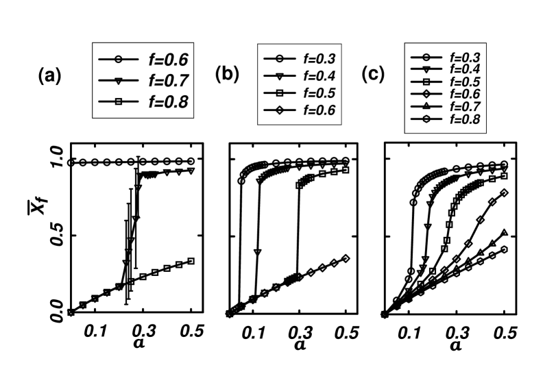
Figure 3: Residual fraction $\bar{x}_{f}$ of living cells versus healing parameter $a$ for several values of the initial stress $f$ at noise level $T=$ (a) 0, (b) 0.2, and (c) 0.4. Note the large error bars in the “transition region” in (a). Error bars in other regions are of the order of the symbol size.

To further investigate this, we plot in fig. 3 the residual fraction $\bar{x}_{f}$ of living cells as a function of $a$ for several values of $f$ and $T$. Figure 3(a) shows $\bar{x}_{f}$ as a function of $a$ for three different values of $f$ near $f_{c}(a=0)=0.677$ at $T=0$. Observed is that sufficiently strong stress (i.e., large values of $f$) in general drives the system out of the healthy state. Otherwise, as $a$ is raised from zero for given value of $f$, $\bar{x}_{f}$ grows from zero and increases sharply around the “critical value” $a_{c}$ depending on $f$, which is reminiscent of a phase transition, say, from the unhealthy to healthy state. The transition appears to become sharper in the presence of noise ($T=0.2$) as shown in fig. 3(b), with $a_{c}$ increasing with $f$. The transition, however, tends to be continuous as the noise level is increased further [see fig. 3(c)].

To confirm these findings, we have carried out Monte Carlo simulations directly and found that the results obtained from 20 independent runs with different initial configurations display perfect agreement with those from numerical integrations of the same samples. In addition, we have also examined the local load sharing case: Direct Monte Carlo simulations of two-dimensional systems, with the load being transferred to the shortest paths, show that qualitative behavior does not change except that the critical stress $f_{c}$ is smaller than that for the system with equal load sharing. Further, as the connectivity of each cell is increased, the behavior approaches that of the latter system [10]. This provides justification for the use of equal load sharing in a biological system, which may have enhanced connectivity in the two- or three-dimensional underlying structure.

In summary, we have introduced a dynamic model for failures in biological organisms and investigated behaviors of the system under stress and healing. The dynamics takes into consideration uncertainty due to imperfections and environmental influences, described by noise. Such noise has been found to result in eventual breakdown of the system without healing. On the other hand, in the presence of healing, the system in general resists stress for a longer time compared with the case of no healing, and avoids complete breakdown. At weak noise the critical stress beyond which the system breaks down increases rapidly with the healing parameter, revealing the crucial role of healing. In spite of simplicity, the model shows quite interesting features, suggestive of the breakdown phenomena in biological systems. Finally, we point out that this model is rather general without details involved and thus provides a convenient starting point for wide potential applicability. In particular many refinements toward more realistic descriptions are conceivable. Corresponding applications to specific biological systems and their implications are left for further study.

- [1] For a review, see, e.g., \Nameda Silveira R. \REVIEWAm. J. Phys.6719991177; \NameCharkrabarti B.K. Benguigui L.G. \BookStatistical Physics of Fracture and Breakdown in Disordered Systems \PublClarendon, Oxford \Year1997.
- [2] \NameDaniels H.E. \REVIEWProc. R. Soc. London, Ser A1831945405; \NamePeirce F.T. \REVIEWJ. Text. Ind.171926355.
- [3] \NameAnderson J.V., Sornette D., Leung K.-t. \REVIEWPhys. Rev. Lett.7819972140; \NameSornette D. \REVIEWJ. Phys. I219922089; \NameZapperi S., Ray P., Stanley H.E. Vespignani A. \REVIEWPhys. Rev. Lett.7819971408.
- [4] \NameColeman B.D. \REVIEWJ. Appl. Phys.291958968; \NameZhang S.-d. \REVIEWPhys. Rev. E5919991589; \NameNewman W.I. Phoenix S.L. \REVIEWPhys. Rev. E632001021507; \NameMoral L., Moreno Y., Gomez J.B. Pacheco A.F. \REVIEWPhys. Rev. E632001066106; \NameKun F., Hidalgo R.C., Hermann H.J. Pal K. \REVIEWPhys. Rev. E672003061802.
- [5] \NameChoi M.Y., Choi J. Yoon B.-G. \REVIEWEurophys. Lett.66200462.
- [6] \NameShim G.M., Choi M.Y. Kim D. \REVIEWPhys. Rev. A4319911079; \NameChoi M.Y. \REVIEWPhys. Rev. Lett.6119882809; \NameLittle W.A. \REVIEWMath. Biosci.191974101.
- [7] \NameHolford N.H.G. Peace K.E. \REVIEWProc. Natl. Acad. Sci. (USA) 89199211466.
- [8] \NamePradhan S. Chakrabarti B.K. \REVIEWPhys. Rev.E672003046124.
- [9] In a real system, however, cells may not be regenerated well in the unhealthy state, namely, as decreases, so does . In fact, if is taken to be this case, the residual fraction , depending on the specific form of , vanishes or becomes much smaller than that in the case of constant .
- [10] \NameYoon B.-G., Choi M.Y. Choi J. \REVIEWUnpublished2005.