Evaluating deterministic policies in two-player iterated games

Abstract

We construct a statistical ensemble of games, where in each independent subensemble we have two players playing the same game. We derive the mean payoffs per move of the representative players of the game, and we evaluate all the deterministic policies with finite memory. In particular, we show that if one of the players has a generalized tit-for-tat policy, the mean payoff per move of both players is the same, forcing the equalization of the mean payoffs per move of both players. In the case of symmetric, non-cooperative and dilemmatic games, we show that generalized tit-for-tat policies together with the condition of not being the first to defect, leads to the highest mean payoffs per move for the players.

Non-Linear Dynamics Group, Instituto Superior Técnico

Department of Physics, Av. Rovisco Pais, 1049-001 Lisboa, Portugal

rui@sd.ist.utl.pt

1 Introduction

Game theory has been formalized by Neumann and Morgenstern in 1944, [1]. Their objective was to introduce into the language of economic theory some mathematical tools for the quantitative analysis of the behaviour of economic agents without a central authority. One of the Neumann and Morgenstern arguments in favour of the usefulness of a theory of games is based on the intrisic limited knowledge about the facts which economists deal with. This argument has also been applied to the description of some physical systems and to evolutionary theories in biology.

In the context of evolutionary biology and in order to analyse the logic of animal conflict, Maynard-Smith [2] introduced a game theory approach to describe some of the evolutionary features of organisms. In the framework of sociology, Axelrod [3] gave several examples where the game theoretical framework is useful. In economics, there is today a vast literature on the applicability of the game theoretical approach to economic decision [4], [5] and [6]. More recently, the same type of formalism has been applied to quantum mechanics [7].

In a game, a policy is a rule of decision for each player, and policies can be deterministic, depending of the previous choices of one or of both players, or can be stochastic. In a two-player non-cooperative game with a finite number of choices or pure strategies, both players know the payoffs, make their choices independently of each other, and know the past history of their choices. It is also assumed that each player maximizes its payoff after a finite or an infinite number of choices or moves.

An important problem is game theory is to determine which policies perform better than others. In this context, Axelrod, [3], proposed the following problem: ”Under what conditions will cooperation emerge in a world of egoists without central authority?”. To help to answer this question a computer tournament has been settled to decide which policy would perform better in an iterated Prisoner’s Dilemma game, introduced by Dresher, Flood and Tucker [8]. The tournament has been won by the tit-for-tat (TFT) policy, submitted by Rapoport, [3, pp. 31]. The TFT policy consists in a simple rule that says that one’s actual move is equal to what the other player did in the previous move.

In fact, several approaches have been developed in order to decide which policies perform better than others in infinitely iterated games. One of these approaches relies on the concept of mixed strategy. In a game with several possible choices or moves, a player has a mixed strategy if he has a probability profile associated to all the possible moves of the game. Based on the concept of mixed strategy, the replicator dynamics approach, [9] and [10], postulates an evolution equation for the probability profiles of each player’s move. This evolution equation implies a precise type of rationality of the players, and the mixed strategy concept has a subjacent infinite memory associated to the choices of the players.

The formal construction of game theory depends on the relation between players and from whom they receive their payoffs. For example, we can formalize a two-player game in such a way that the payoffs won by one player are the losses of the other, [11]. Another approach is to consider that the player’s payoffs are obtained from external sources. Our construction applies to the second case and applies to games describing the global behaviour of systems from economy, sociology and evolutionary biology.

The aim of this paper is to derive the mean payoffs of the ’representative players’ of a game, and to formulate the problem of deciding which policy performs better than another in iterated non-cooperative games.

This paper is organized as follows. In Section 2, we introduce some of the definitions that will be used along this paper, and we analyse and interpret iterated non-cooperative games from the point of view of dynamical system theory. In order to evaluate games and deterministic strategies with finite memory, we take the point of view of uniform ensembles of statistical mechanics and we introduce the concept of representative ensemble of a game. In this context, the players of the infinite set of games are substituted by the ’representative agents’ of the game.

In Section 3, we consider the case of a uniform ensemble of games, where in each subensemble we have two players playing the same game. The mean value of the payoffs per move taken over the uniform ensemble is calculated, and gives information about the performance of a game. In Section 4, we evaluate the performance of deterministic strategies with finite memory length. In the case where in each subensemble a player has a deterministic strategy and the other makes his choices with equal probabilities, we calculate the ensemble averages of the payoffs per move. The main results of sections 3 and 4 are summarized in Theorems 3.1 and 4.1, and Corollary 4.2. In particular, we show that if one of the players has a generalized tit-for-tat policy, the mean payoff per move of both players is the same. Therefore, generalized tit-for-tat is the best policy against exploitation.

In Section 5, we consider the case where the opponent players have deterministic policies, within the same memory class. In this case, the game dynamics is a deterministic process, and the mean payoffs per move depend on the initial moves of both players and on the policy functions of both players. Comparing all the possible deterministic strategies with memory length $1$, we prove that, in dilemmatic games, the generalized tit-for-tat policy together with the condition of not being the first to defect, leads to the highest possible mean payoffs per move for the players.

In Section 6, we apply the formalism developed in this paper to the Prisoner’s Dilemma and to the Hawk-Dove games, and we analyse their state space structure. Finally, in Section 7, we summarize the main conclusions of the paper.

2 Formalism and definitions

We take a two-player game with two possible choices or moves — two pure strategies. At times $n\geq 1$, each player chooses, independently of the other, one of the two possible pure strategies. These pure strategies are represented by the symbols ’0’ and ’1’. We denote by ${\bf S}=\{0,1\}$ the set of pure strategies, and by $P$ and $Q$ the two players. After a move, each player owns a profit or payoff that is dependent of the opponent move. The payoff matrices of the game are:

$$A=\left(\begin{array}[]{cc}A_{00}&A_{01}\\ A_{10}&A_{11}\end{array}\right)\,,\quad B=\left(\begin{array}[]{cc}B_{00}&B_{01}\\ B_{10}&B_{11}\end{array}\right)$$

where the payoff of $P$ is $A_{ij}$ if player $P$ plays $i$ and $Q$ plays $j$. In the same move, $Q$ has payoff $B_{ij}$. If each player makes its choice independently of the other, we are in the context of non-cooperative games. If $B=A^{T}$, the two-player game is symmetric. In the following, we analyze only the case of symmetric and non-cooperative games.

In a two-player symmetric game, we say that a pure strategy $i\in{\bf S}$ is dominant, [12], if $A_{ij}\geq A_{kj}$, for every $j=0,1$, and $A_{ij}>A_{kj}$ for some $j$ and $k\not=i$. For example, the symmetric and non-cooperative games with payoff matrices,

$$A_{1}=\left(\begin{array}[]{cc}3&0\\ 5&1\end{array}\right)\,,\quad A_{2}=\left(\begin{array}[]{cc}1&0\\ 5&3\end{array}\right)$$

have ’1’ as dominant strategy ($A_{10}>A_{00}$ and $A_{11}>A_{01}$). In the first game, if the two players choose both the dominant strategy ’1’, their payoffs is $1$. In the second game, the payoff of each players is $3$, and the dominant strategy is the right choice for both players. However, as $A_{00}>A_{11}$ for the first game, if both players choose the non-dominant strategy, their individual payoffs per move is higher when compared with the choice of the dominant strategy by both players.

These two examples suggest the following definition: A symmetric two-player game is dilemmatic, if either,

$$A_{10}>A_{00}>A_{11}>A_{01}\quad\hbox{and}\quad 2A_{00}>A_{01}+A_{10}$$

or,

$$A_{01}>A_{11}>A_{00}>A_{10}\quad\hbox{and}\quad 2A_{11}>A_{10}+A_{01}$$

where the second inequalities in (2.1) and (2.2) have been introduced in order to favour the non-dominant strategy.

In the first case of a dilemmatic game, (2.1), the strategy ’1’ is dominant. In the second case, (2.2), ’0’ is the dominant strategy. If both players choose the dominant strategy in one move, they get smaller payoffs than the ones they could have obtained if both had chosen the non-dominant strategy.

In an iterated game with a fixed payoff matrix, players are always playing the same game, and their payoffs accumulate. Therefore, a two-player iterated game is described by the two sequences of pure strategies of each player,

$$\begin{array}[]{l}{\bf\mu}=(\mu_{1},\mu_{2},\ldots,\mu_{n},\ldots)\\ {\bf\sigma}=(\sigma_{1},\sigma_{2},\ldots,\sigma_{n},\ldots)\end{array}$$

where $\mu_{n}$ and $\sigma_{n}$ represent the choices of the players $P$ and $Q$, respectively, at discrete time $n\geq 1$, and $\mu_{n},\sigma_{n}\in{\bf S}$. The sequences (2.3), completely specify the accumulated payoffs of both players. We call ${\bf\mu}$ and ${\bf\sigma}$ the game record sequences. In an infinitely iterated game, the accumulated payoff of the players can be infinite. The mean payoffs per move are always finite and, for a symmetric game, they are given by,

$$\begin{array}[]{l}G_{p}=\lim_{n\to\infty}{1\over n}\sum_{i=1}^{n}A_{\mu_{i}\sigma_{i}}\\ G_{q}=\lim_{n\to\infty}{1\over n}\sum_{i=1}^{n}A_{\sigma_{i}\mu_{i}}\end{array}$$

where $G_{p}$ and $G_{q}$ are the mean payoffs of players $P$ and $Q$, respectively.

An example of a symmetric, non-cooperative, and dilemmatic game is the Prisoner’s Dilemma game. In this game, we have two players with two possible pure strategies, ’0’ and ’1’, and we have chosen the payoff matrix,

$$A=\left(\begin{array}[]{cc}3&-9\\ 11&-5\end{array}\right)$$

As, $A_{10}>A_{00}>A_{11}>A_{01}$ and $2A_{00}>A_{01}+A_{10}$, the Prisoner’s Dilemma game is dilemmatic with ’1’ as dominant pure strategy. The pure strategy ’0’ corresponds to cooperation and the pure strategy ’1’ to defection. For a discussion about the importance of dilemmatic games and the Prisoner’s Dilemma game, see the discussion in Axelrod, [3].

Following Neumann and Morgenstern [1], a strategy or policy is a set of rules that tells each participant how to behave in every situation which may arise. The only sources of information available to the players is the set of all possible moves, their possible payoffs, and the history of the previous moves of both players. To describe a rule of decision, policy, or strategy we can adopt the Neumann-Morgenstern view where a rule of decision is specified through the knowledge of a function of the $m$ previous moves.

Deterministic strategy: In an iterated two-player game, with game records ${\bf\mu}$ and ${\bf\sigma}$ for players $P$ and $Q$, respectively, a rule of decision or a deterministic strategy with memory length $m\geq 1$ for player $P$ is a function $f:{\bf S}^{m}\to{\bf S}$ such that,

$$\mu_{i}=f(\sigma_{i-m},...,\sigma_{i-1})$$

for every $i>m$. Analogously, player $Q$ has a deterministic strategy with memory length $n\geq 1$, if there exists a function $g:{\bf S}^{n}\to{\bf S}$ such that,

$$\sigma_{i}=g(\mu_{i-n},...,\mu_{i-1})$$

for every $i>n$.

In the following, deterministic policy and deterministic strategy have the same meaning. In some game theory texts, the word ’strategy’ refers to ’pure strategy’, an element of the set ${\bf S}=\{0,1\}$, and in other contexts if refers to policies, as in ’tit-for-tat strategy’.

By definition, the outcome of a player’s choice or move at time $i\geq m+1$ is determined by a finite number of previous moves of the other. In general, we can take the functions $f:{\bf S}^{m+n}\to{\bf S}$ and $g:{\bf S}^{r+s}\to{\bf S}$, and set,

$$\begin{array}[]{l}\mu_{i}=f(\sigma_{i-m},...,\sigma_{i-1},\mu_{i-n},...,\mu_{i-1})\\ \sigma_{i}=g(\mu_{i-r},...,\mu_{i-1},\sigma_{i-s},...,\sigma_{i-1})\end{array}$$

In the following we will only analyze the case where each player’s choice depends on a finite number of previous moves of the other, and $m=n$.

For example, adopting the definition of the tit-for-tat (TFT) strategy given in the introduction, a TFT strategy with memory length $m=1$ is described by the boolean identity function $f:{\bf S}\to{\bf S}$, defined by,

$$f(0)=0\qquad\hbox{and}\qquad f(1)=1$$

Generalized tit-for-tat strategy (GTFT): We say that $f:{\bf S}^{m}\to{\bf S}$ is a generalized tit-for-tat strategy with memory length $m$, if the number of ’0’ and ’1’ in $f({\bf\sigma}^{(m)})$, when ${\bf\sigma}^{(m)}$ runs over the set ${\bf S}^{m}$, are equal. More formally, $f:{\bf S}^{m}\to{\bf S}$ is a generalized tit-for-tat strategy with memory length $m$, if,

$$\#\{{\bf\sigma}^{(m)}\in{\bf S}^{m}:f({\bf\sigma}^{(m)})=0\}=\#\{{\bf\sigma}^{(m)}\in{\bf S}^{m}:f(\sigma^{(m)})=1\}$$

where ${\bf\sigma}^{(m)}=(\sigma_{1},\ldots,\sigma_{m})$, and $\sigma_{i}\in{\bf S}$.

To solve a game it is meant to find a procedure to determine for each player’s choice which is the most favourable result ([1], [11] and [13]). In this context, the concepts of mixed strategy and equilibrium state of a game are fundamental tools in game theory.

A mixed strategy is a collection of probabilities associated to each player and its pure strategies. The players $P$ and $Q$ have mixed strategies $s_{p}=(s_{0p},s_{1p})$ and $s_{q}=(s_{0q},s_{1q})$, if each player plays pure strategy $i$ with probability $s_{i*}$. Obviously, $s_{0*}+s_{1*}=1$.

In a symmetric game with two pure strategies and mixed strategies $s_{p}$ and $s_{q}$ for players $P$ and $Q$, respectively, the mean payoffs per move of players $P$ and $Q$ are,

$$\begin{array}[]{ll}P:\quad E(s_{p}|s_{q})&=s_{0p}(s_{0q}A_{00}+s_{1q}A_{01})+s_{1p}(s_{0q}A_{10}+s_{1q}A_{11})\\ &=s_{0p}s_{0q}A_{00}+s_{0p}s_{1q}A_{01}+s_{1p}s_{0q}A_{10}+s_{1p}s_{1q}A_{11}\\ Q:\quad E(s_{q}|s_{p})&=s_{0q}(s_{0p}A_{00}+s_{1p}A_{01})+s_{1q}(s_{0p}A_{10}+s_{1p}A_{11})\\ &=s_{0q}s_{0p}A_{00}+s_{0q}s_{1p}A_{01}+s_{1q}s_{0p}A_{10}+s_{1q}s_{1p}A_{11}\end{array}$$

The time evolution of a game with mixed strategies $s_{p}$ and $s_{q}$ can be seen as a stochastic processes with two independent random variables $X$ and $Y$. The random variables $X$ and $Y$, associated to players $P$ and $Q$, respectively, have mean values given by (2.7). More precisely, $X$ can assume the values $A_{00}$, $A_{01}$, $A_{10}$, $A_{11}$ with probabilities $s_{0p}s_{0q}$, $s_{0p}s_{1q}$, $s_{1p}s_{0q}$ and $s_{1p}s_{1q}$, respectively. Analogously, $Y$ takes values in the same set, with probabilities: $s_{0q}s_{0p}$, $s_{0q}s_{1p}$, $s_{1q}s_{0p}$ and $s_{1q}s_{1p}$. Therefore, the deviations from the mean payoffs per move of the players, or the fluctuations from the mean values, are characterised by the variances,

$$\begin{array}[]{ll}\sigma^{2}_{p}(s_{p}|s_{q})&=s_{0p}s_{0q}(A_{00}-E(s_{p}|s_{q}))^{2}+s_{0p}s_{1q}(A_{01}-E(s_{p}|s_{q}))^{2}\\ &+s_{1p}s_{0q}(A_{10}-E(s_{p}|s_{q}))^{2}+s_{1p}s_{1q}(A_{11}-E(s_{p}|s_{q}))^{2}\\ \sigma^{2}_{q}(s_{q}|s_{p})&=s_{0q}s_{0p}(A_{00}-E(s_{q}|s_{p}))^{2}+s_{0q}s_{1p}(A_{01}-E(s_{q}|s_{p}))^{2}\\ &+s_{1q}s_{0p}(A_{10}-E(s_{q}|s_{p}))^{2}+s_{1q}s_{1p}(A_{11}-E(s_{q}|s_{p}))^{2}\end{array}$$

In general, $E(s_{p}|s_{q})\not=E(s_{q}|s_{p})$, but, by a straightforward calculation, $\sigma^{2}_{p}(s_{p}|s_{q})=\sigma^{2}_{q}(s_{q}|s_{p})$.

Imposing the condition $E(s_{p}|s_{q})=E(s_{q}|s_{p})$ in (2.7), a game or a mixed strategy is equalitarian, if either, $A_{01}=A_{10}$, or $s_{p}=s_{q}$.

To characterise the dynamics of an iterated symmetric game, we introduce the concept of phase or state space of a game. The state space of a two-player game is the convex closure of the points $(A_{00},A_{00})$, $(A_{11},A_{11})$, $(A_{01},A_{10})$ and $(A_{10},A_{01})$, in the two-dimensional space of the payoffs of players $P$ and $Q$. Let us denote by ${\mathcal{K}}$ the state space of a game. As $s_{0p},s_{0q}\in[0,1]$, then $(E(s_{p}|s_{q}),E(s_{q}|s_{p}))\in{\mathcal{K}}$. In Fig. 1, we show the state space ${\mathcal{K}}$ for the Prisoner’s Dilemma game with payoff matrix (2.5).

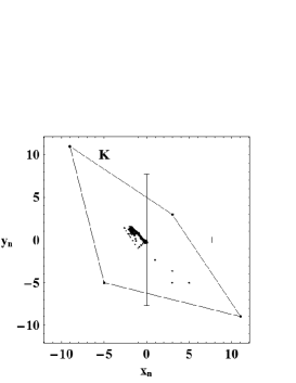
Figure 1: State space ${\mathcal{K}}$ of the Prisoner’s Dilemma game with payoff matrix (2.5), where $x_{n}$ and $y_{n}$ are the mean payoffs per move of players $P$ and $Q$, as calculated from (2.9). The dots represent the mean payoff per move of an instance of the iterated game with both players choosing strategies ’0’ and ’1’ with equal probabilities ($s_{p}=s_{q}=1/2$). By (2.7), the equilibrium of the game is the point $(0,0)$, and the standard deviations of the mean payoffs of the players are $\sigma_{p}=\sigma_{q}=\sqrt{59}=7.68$, calculated from (2.8).

In an iterated game, the mean initial (at time $n=1$) payoffs per move of both players is $(x_{1},y_{1})=(A_{\mu_{1}\sigma_{1}},A_{\sigma_{1}\mu_{1}})\in{\mathcal{K}}$. By (2.4) and after $n+1$ moves, the mean payoffs per move of both players is,

$$\begin{array}[]{ll}(x_{n+1},y_{n+1})&=({1\over{n+1}}\sum_{i=1}^{n+1}A_{\mu_{i}\sigma_{i}},{1\over{n+1}}\sum_{i=1}^{n+1}A_{\sigma_{i}\mu_{i}})\\ &=({n\over{n+1}}x_{n}+{1\over{n+1}}A_{\mu_{n+1}\sigma_{n+1}},{n\over{n+1}}y_{n}+{1\over{n+1}}A_{\sigma_{n+1}\mu_{n+1}})\in{\mathcal{K}}\end{array}$$

and the iterated two-player game is dynamically described by a (non-deterministic) one-to-many map, $\beta:{\mathcal{K}}\to{\mathcal{K}}$, [14]. The equilibrium point or equilibrium solution of a game is the point $\lim_{n\to\infty}(x_{n},y_{n})$.

For a given mixed strategy profile $s_{p}$ and $s_{q}$ of players $P$ and $Q$, the iterated two-player game has the equilibrium point, $(E(s_{p}|s_{q}),E(s_{q}|s_{p}))\in{\mathcal{K}}$. As $s_{0p},s_{0q}\in[0,1]$, the set of equilibrium states of the map $\beta:{\mathcal{K}}\to{\mathcal{K}}$ span all the state space of a game.

For example, in a two-player game with the mixed strategy profiles $s_{p}=(1/2,1/2)$ and $s_{q}=(1/2,1/2)$, by (2.7), the equilibrium point of the game is,

$$({1\over 4}(A_{00}+A_{01}+A_{10}+A_{11}),{1\over 4}(A_{00}+A_{01}+A_{10}+A_{11}))$$

By (2.8), the fluctuations around the equilibrium are,

$$\begin{array}[]{ll}&\sigma^{2}_{p}((1/2,1/2)|(1/2,1/2))=\sigma^{2}_{q}((1/2,1/2)|(1/2,1/2))\\ &={1\over 4^{2}}\left(3A_{00}^{2}+3A_{01}^{2}+3A_{10}^{2}+3A_{11}^{2}\right.\\ &\left.-2A_{00}(A_{01}+A_{10}+A_{11})-2A_{11}(A_{01}+A_{10})-2A_{01}A_{10}\right)\end{array}$$

In Fig. 1, we represent several iterates of the map $\beta$ for the Prisoner’s Dilemma game with payoff matrix (2.5), and mixed strategies $s_{p}=s_{p}=(1/2,1/2)$. In the limit $n\to\infty$, $(x_{n},y_{n})\to(0,0)$. The fluctuations from equilibrium have standard deviations $\sigma_{p}=\sigma_{q}=\sqrt{59}=7.68$.

A mixed strategy is a strict Nash equilibrium solution of a game if $P$ and $Q$ maximizes their payoffs per move independently of each other. A mixed strategy is a Nash bargain equilibrium solution of a game if $E(s_{p}|s_{p})$ is a maximum.

In the case of the of the Prisoner’s Dilemma game with payoff matrix (2.5), by (2.7), we have,

$$\begin{array}[]{ll}P&:\quad E(s_{p}|s_{q})=-5-4s_{0p}+16s_{0q}-4s_{0p}s_{0q}\\ Q&:\quad E(s_{q}|s_{p})=-5-4s_{0q}+16s_{0p}-4s_{0p}s_{0q}\end{array}$$

Maximizing $E(s_{p}|s_{q})$ in order to $s_{0p}$ and $E(s_{q}|s_{p})$ in order to $s_{0q}$, the strict Nash equilibrium of the game is obtained when both player choose the mixed strategy $(s_{0p},s_{1p})=(s_{0p},s_{1p})=(0,1)$. In this case, the Nash equilibrium state of the map $\beta:{\mathcal{K}}\to{\mathcal{K}}$ is the point $(-5,-5)\in{\mathcal{K}}$. The Nash bargain solution of the game is obtained from (2.12) with $s_{p}=s_{q}$, and is the point $(3,3)\in{\mathcal{K}}$, Fig. 1. As both Nash solutions correspond to the choices of pure strategies with probability 1, by (2.8), the fluctuations of the iterated game have zero standard deviations. In general, a n-person non-cooperative game has always a strict Nash equilibrium, [13].

The choice of a mixed strategy profile for a game has the advantage that the iterates of the map $\beta:{\mathcal{K}}\to{\mathcal{K}}$ converges to the equilibrium solution $E(s_{p}|s_{q})$. However, the choice of a mixed strategy profile implies that both players have infinite memory, which, in real situations, is difficult or even impossible to fulfil.

On the other hand, in some game theory approaches describing the global behaviour of economic, social and evolutionary systems, there are a large number of agents or players in mutual interaction. These individual agents interact with the same rules and can also change partners along time. These situations are difficult to interpret under the infinite memory hypothesis, implicitly associated to the concept of mixed strategies.

Following this point of view, to evaluate a non-cooperative and symmetric game and their possible deterministic strategies (short memory), we adopt the point of view of the statistical ensembles of statistical mechanics. We suppose first that we have an infinite system composed by independent subensembles, where in each subensemble we have two players playing the same game with payoff matrix $A$. We call this ensemble of independent games the uniform ensemble ([15, pp. 56]) of the game. This uniform ensemble is characterized by the payoff matrix $A$, and the players $P$ and $Q$ are the representative agents of the ensemble of the game.

In each subensemble, a game with payoff matrix $A$ is played, and subensembles are characterized by the mean payoffs per move of both players. The global properties of the game will be described by the mean payoffs per move averaged over all the subensembles. We say that the representative players $P$ and $Q$ of the game have mean payoffs per move ${\bar{G}}_{p}$ and ${\bar{G}}_{q}$, respectively, where the average is taken over all the subensembles.

To evaluate a game, we first consider that each player chooses its pure strategies with equal probabilities, and each subensemble is characterized by the two sequences of pure strategies $\mu$ and $\sigma$. The properties of the game are determined by ${\bar{G}}_{p}$ and ${\bar{G}}_{q}$.

To evaluate a deterministic strategy or policy, we consider that in each subensemble game, $P$ plays with the deterministic policy $f$, and $Q$ has a game record ${\bf\sigma}\in{\bf S}^{\hbox{{\amss\char 78\relax}}}$. Defining an ensemble probability density function $\rho_{q}$ for the occurrence of game record ${\bf\sigma}$ for player $Q$, the ensemble of games will by characterized by the mean payoff per move of both players averaged over the set of all allowed sequences ${\bf\sigma}\in{\bf S}^{\hbox{{\amss\char 78\relax}}}$ with probability measure $\rho_{q}$. These averages depend on $f$ and $\rho_{q}$, and we can compare the performance of a policy with the case where the players have no policies. Within the same memory class, we use these ensemble averages to compare the mean payoffs for different policies.

When both players have a deterministic policy, the mean payoffs per move of the players depend on the finite number of initial conditions of the game.

3 The uniform ensemble of a game

We consider an ensemble of subsystems, where in each subsystem there are two players playing the same game. We denote the game record of players $P$ and $Q$ by ${\bf\mu}$ and ${\bf\sigma}$, respectively. As ${\bf\mu}$ and ${\bf\sigma}$ are infinite sequences of ’0’ and ’1’, we can identify ${\bf\mu}$ and ${\bf\sigma}$ as real numbers in the interval $[0,1]$ through,

$$x=\sum_{i=1}^{\infty}{\mu_{i}\over 2^{i}}\ ,\qquad y=\sum_{i=1}^{\infty}{\sigma_{i}\over 2^{i}}$$

Relations (3.1) define a map $\phi:{\bf S}^{\hbox{{\amss\char 78\relax}}}\rightarrow[0,1]$. The map $\phi$ is an isomorphism, except when $(\sigma_{1},\sigma_{2},...)$ or $(\mu_{1},\mu_{2},...)$ represents dyadic rational numbers, [16]. As the set of dyadic rationals has zero Lebesgue measure, the infinite sequence of moves of both players can be represented, almost everywhere, by two real numbers $x,y\in[0,1]$. Therefore, the interval $[0,1]$ is naturally the space of game records.

Making this identification between game records and real numbers, in each subensemble game, by (2.4), the mean payoffs per move of the players are,

$$\begin{array}[]{ll}G_{p}({\bf\mu},{\bf\sigma})&=\lim_{n\to\infty}{1\over n}\sum_{i=1}^{n}A_{\mu_{i}\sigma_{i}}:=G_{p}(x,y)\cr G_{q}({\bf\mu},{\bf\sigma})&=\lim_{n\to\infty}{1\over n}\sum_{i=1}^{n}A_{\sigma_{i}\mu_{i}}:=G_{q}(x,y)\end{array}$$

where $x,y\in[0,1]$.

As each subensemble game is independent of the other, and each player’s move is independent of the history of the game, we can assign ensemble probability density functions to the game records. Let $\rho_{p}(x)$ and $\rho_{q}(y)$ be the ensemble probability density functions of game records of the representative players $P$ and $Q$, respectively. For example, $\rho_{p}(x)dx$ is the probability of finding a subensemble with player $P$ with a game record in an interval of length $dx$ centred around $x$.

Assuming further that all the game records are equally probable, $\rho_{p}(x)=1$ and $\rho_{q}(y)=1$, the ensemble averages of the mean payoffs per move are,

$$\begin{array}[]{ll}{\bar{G}}_{p}&=\int_{0}^{1}\int_{0}^{1}G_{p}(x,y)\rho_{p}(x)\rho_{q}(y)dx\,dy=\int_{0}^{1}\int_{0}^{1}G_{p}(x,y)dx\,dy\\ {\bar{G}}_{q}&=\int_{0}^{1}\int_{0}^{1}G_{q}(x,y)\rho_{p}(x)\rho_{q}(y)dx\,dy=\int_{0}^{1}\int_{0}^{1}G_{q}(x,y)dx\,dy\end{array}$$

To characterize the statistical ensemble of a non-cooperative and symmetric game with payoff matrix $A$, we now calculate the integrals in (3.3). We consider the sequences of functions,

$$\begin{array}[]{ll}G_{p}^{n}({\bf\mu},{\bf\sigma})&={1\over n}\sum_{i=1}^{n}A_{\mu_{i}\sigma_{i}}\\ G_{q}^{n}({\bf\mu},{\bf\sigma})&={1\over n}\sum_{i=1}^{n}A_{\sigma_{i}\mu_{i}}\end{array}$$

As $n\to\infty$, $G_{p}^{n}({\bf\mu},{\bf\sigma})\to G_{p}({\bf\mu},{\bf\sigma})$, and $G_{q}^{n}({\bf\mu},{\bf\sigma})\to G_{q}({\bf\mu},{\bf\sigma})$. In the sense of Lebesgue integration, the integrals in (3.3) can be calculated as the limits of the integrals of the functions $G_{p}^{n}({\bf\mu},{\bf\sigma})$ and $G_{q}^{n}({\bf\mu},{\bf\sigma})$.

Let us first take $n=1$. By (3.2), (3.3) and (3.4), we have,

$$\begin{array}[]{ll}{\bar{G}}_{p}^{1}&=\int_{0}^{1}\int_{0}^{1}A_{\mu_{1}\sigma_{1}}dx\,dy\\ {\bar{G}}_{q}^{1}&=\int_{0}^{1}\int_{0}^{1}A_{\sigma_{1}\mu_{1}}dx\,dy\end{array}$$

where $\mu_{1}$ and $\sigma_{1}$ are the first digits in the binary developments of $x$ and $y$, both in the interval $[0,1]$. Therefore, the functions $A_{\mu_{1}\sigma_{1}}\equiv A_{\mu_{1}\sigma_{1}}(x,y)$ and $A_{\sigma_{1}\mu_{1}}\equiv A_{\sigma_{1}\mu_{1}}(x,y)$ are piecewise constant in the unit square, and the integrals in (3.5) are straightforwardly evaluated to,

$$\begin{array}[]{ll}{\bar{G}}_{p}^{1}&=\int_{0}^{1}\int_{0}^{1}A_{\mu_{1}\sigma_{1}}dx\,dy={1\over 2^{2}}(A_{00}+A_{01}+A_{10}+A_{11})\\ {\bar{G}}_{q}^{1}&=\int_{0}^{1}\int_{0}^{1}A_{\sigma_{1}\mu_{1}}dx\,dy={1\over 2^{2}}(A_{00}+A_{01}+A_{10}+A_{11})\end{array}$$

Note that, the functions $A_{\mu_{1}\sigma_{1}}(x,y)$ and $A_{\sigma_{1}\mu_{1}}(x,y)$ are piecewise constant functions from $[0,1]\times[0,1]$ to the set $\{A_{00},A_{01},A_{10},A_{11}\}$.

In general, by (3.4) and (3.3),

$$\begin{array}[]{ll}{\bar{G}}_{p}^{n+1}&={n\over n+1}{\bar{G}}_{p}^{n}+{1\over n+1}\int_{0}^{1}\int_{0}^{1}A_{\mu_{n+1}\sigma_{n+1}}dx\,dy\\ {\bar{G}}_{q}^{n+1}&={n\over n+1}{\bar{G}}_{q}^{n}+{1\over n+1}\int_{0}^{1}\int_{0}^{1}A_{\sigma_{n+1}\mu_{n+1}}dx\,dy\end{array}$$

The functions $A_{\mu_{n}\sigma_{n}}\equiv A_{\mu_{n}\sigma_{n}}(x,y)$ and $A_{\sigma_{n}\mu_{n}}\equiv A_{\sigma_{n}\mu_{n}}(x,y)$ are piecewise constant and assume the constant values $A_{00}$, $A_{01}$, $A_{10}$ and $A_{11}$ in squares of side $1/2^{n}$. As, for each pair of indices $(\sigma_{n},\mu_{n})$, the domain where $A_{\sigma_{n}\mu_{n}}(x,y)$ is constant is composed by $2^{2(n-1)}$ disjoint squares, we have,

$$\begin{array}[]{ll}\int_{0}^{1}\int_{0}^{1}A_{\mu_{n}\sigma_{n}}dx\,dy&=\int_{0}^{1}\int_{0}^{1}A_{\sigma_{n}\mu_{n}}dx\,dy\\ &={2^{2(n-1)}\over 2^{2n}}(A_{00}+A_{01}+A_{10}+A_{11})\\ &={1\over 2^{2}}(A_{00}+A_{01}+A_{10}+A_{11})\end{array}$$

Introducing (3.8) into (3.7), by induction, and taking the limit $n\to\infty$, we obtain the values of the ensemble average of the mean payoffs per move of each player:

Theorem 3.1.

We consider an ensemble of non-cooperative and symmetric two-player game, where in each subensemble we have two players making their choices with equal probabilities. Assume that each player’s move is independent of the history of the game and that the ensemble probability density functions of each representative player are uniform in the interval $[0,1]$ of the game records. Then, the mean payoffs per move of the representative players of the game are equal and are given by,

$${\bar{G}}_{p}={\bar{G}}_{q}={1\over 2^{2}}(A_{00}+A_{01}+A_{10}+A_{11})$$

where the $A_{ij}$ are the entries of the payoff matrix.

In the uniform statistical ensemble of a non-cooperative and symmetric game with all the players choosing their pure strategies with equal probabilities, the average payoff per move is equal to the average value of the entries of the payoff matrix $A$.

These elementary results can be straightforwardly generalized to non-cooperative and non-symmetric $n$-player games.

4 Evaluating deterministic strategies

To evaluate the performance of a deterministic strategy in an iterated game, we first enumerate the class of all the boolean functions $f:{\bf S}^{m}\rightarrow{\bf S}$, where ${\bf S}=\{0,1\}$. These boolean functions describe all the possible deterministic strategies.

For each class of functions with memory length $m$, there are exactly $2^{2^{m}}$ different functions. To enumerate a deterministic policy function within a memory class $m$, $f({{\bf\sigma}}^{(m)})$, where ${{\bf\sigma}}^{(m)}=(\sigma_{1},\ldots,\sigma_{m})\in\{0,1\}^{m}$, we introduce an additional index $n$. Within each memory class $m$, each possible policy function will be denoted by $f_{m,n}$, where $n=\sum_{i=0}^{2^{m}-1}f_{m,n}({{\bf\sigma}}^{(m)}_{i})2^{i}$ is the policy number, ${{\bf\sigma}}^{(m)}_{i+1}={{\bf\sigma}}^{(m)}_{i}+(0,0,\ldots,1)$, ${{\bf\sigma}}^{(m)}_{0}=(0,0,\ldots,0)$, and the ”plus” symbols must be understood in the sense of binary arithmetic. For example, in Table 1, we show all the possible deterministic policy functions with memory length $m=1$.

$f_{1,n}(0)$ $f_{1,n}(1)$ $f_{1,0}$ 0 0 $f_{1,1}$ 1 0 $f_{1,2}$ 0 1 $f_{1,3}$ 1 1

Table 1: Deterministic policy functions for $m=1$.

In this case, the deterministic TFT policy corresponds to the boolean function $f_{1,2}$. The functions $f_{1,2}$ and $f_{1,1}$ are GTFT policies with memory length $m=1$.

Suppose now that the representative player $P$ of a game has a policy $f_{m,n}$ and the opponent player $Q$ can have any game sequence $\sigma=(\sigma_{1},\sigma_{2},...)$. Then, by (2.4), for the infinitely iterated game, the mean payoff per move for each player is,

$$\begin{array}[]{ll}G_{p}({\bf\sigma})&=\lim_{M\to\infty}{1\over M}\sum_{i=1}^{M}A_{\mu_{i}\sigma_{i}}\\ &=\lim_{M\to\infty}{1\over M-m}\sum_{i=m+1}^{M}A_{f_{m,n}(\sigma_{i-m},...,\sigma_{i-1})\sigma_{i}}\\ G_{q}({\bf\sigma})&=\lim_{M\to\infty}{1\over M-m}\sum_{i=m+1}^{M}A_{\sigma_{i}f_{m,n}(\sigma_{i-m},...,\sigma_{i-1})}\end{array}$$

and $G_{p}$ and $G_{q}$ are functions of ${\bf\sigma}=(\sigma_{1},\sigma_{2},...)$ and $f_{m,n}$. In the first $m$ iterations of the game, the accumulated mean payoffs depend on the initial choices of the players. However, in the limit $M\to\infty$, the dependence on the initial choices vanishes.

Let us take the infinite sequence $(\sigma_{1},\sigma_{2},...)\in{\bf S}^{\hbox{{\amss\char 78\relax}}}$ characterizing one of the possible outcomes of the choices of the player $Q$, and define the real number,

$$y=\sum_{i=1}^{\infty}{\sigma_{i}\over 2^{i}}$$

With this identification between infinite sequences of zeros and ones with real numbers in the interval $[0,1]$, we write the mean payoffs as,

$$\begin{array}[]{l}G_{p}({\bf\sigma})\equiv G_{p}(y;f_{m,n}):=P_{m,n}(y)\\ G_{q}({\bf\sigma})\equiv G_{q}(y;f_{m,n}):=Q_{m,n}(y)\end{array}$$

Let us suppose now that we are in framework of statistical mechanics and we have an ensemble or collectivity of players $P$ and $Q$. In each subensemble of the collectivity, the player $P$ plays according to strategy $f_{m,n}$ and $Q$ has some game record $y\in[0,1]$. Suppose additionally that all the subensembles of the collectivity are independent.

As each member of the collectivity is independent of the others, we can assign an ensemble density function $\rho_{q}(y)$ to the collectivity. The function $\rho_{q}(y)$ is the probability density of the game record $y$ of player $Q$. If $\rho_{q}(y)=1$, all the game records of $Q$ are equally probable. The uniform ensemble of the game can then be characterized by the ensemble mean payoffs per move and per player,

$$\begin{array}[]{ll}{\bar{P}}_{m,n}&=\int_{0}^{1}P_{m,n}(y)\rho_{q}(y)dy=\int_{0}^{1}P_{m,n}(y)dy\\ {\bar{Q}}_{m,n}&=\int_{0}^{1}Q_{m,n}(y)\rho_{q}(y)dy=\int_{0}^{1}Q_{m,n}(y)dy\end{array}$$

In Fig. 2, we show the mean payoff functions $P_{m,n}(y)$ and $Q_{m,n}(y)$ for the TFT policy $f_{1,2}$ and payoff matrix (2.5) of the Prisoner’s Dilemma game. These functions have been calculated numerically from (4.1), (4.2) and (4.3).

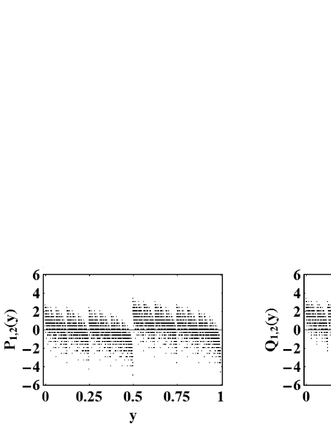
Figure 2: Mean payoffs per move $P_{1,2}(y)$ and $Q_{1,2}(y)$ as a function of the game record $y\in[0,1]$ of the player $Q$, in the Prisoner’s Dilemma game with payoff matrix (2.5). Player $P$ has TFT policy $f_{1,2}$.

To calculate the mean payoffs ${\bar{P}}_{m,n}$ and ${\bar{Q}}_{m,n}$ given by (4.4), we first approximate the functions $P_{m,n}(y)$ and $Q_{m,n}(y)$ by sequences of piecewise constant functions. By (4.1)-(4.3), we define the sequences of functions, $\{P_{m,n}^{M}(y)\}_{M\geq m+1}$ and $\{Q_{m,n}^{M}(y)\}_{M\geq m+1}$, as,

$$\begin{array}[]{ll}P_{m,n}^{M}(y)&={1\over M-m}\sum_{i=m+1}^{M}A_{f_{m,n}(\sigma_{i-m},...,\sigma_{i-1})\sigma_{i}}\\ Q_{m,n}^{M}(y)&={1\over M-m}\sum_{i=m+1}^{M}A_{\sigma_{i}f_{m,n}(\sigma_{i-m},...,\sigma_{i-1})}\end{array}$$

where $(\sigma_{1},\sigma_{2},...)$ is the binary development of $y$. For $M\geq m+1$, $P_{m,n}^{M}(y)$ and $Q_{m,n}^{M}(y)$ are piecewise constant functions in the interval $[0,1]$, and, in the limit $M\to\infty$, they converge almost everywhere to $P_{m,n}(y)$ an $Q_{m,n}(y)$, Fig. 2. In the sense of Lebesgue integrations, this implies that,

$$\begin{array}[]{l}\lim_{M\to\infty}\int_{0}^{1}P_{m,n}^{M}(y)dy={\bar{P}}_{m,n}\\ \lim_{M\to\infty}\int_{0}^{1}Q_{m,n}^{M}(y)dy={\bar{Q}}_{m,n}\end{array}$$

Let us now calculate the integrals in (4.6). For $M=m+1$, by (4.5), we have,

$$\begin{array}[]{ll}P_{m,n}^{m+1}(y)&=A_{f_{m,n}(\sigma_{1},...,\sigma_{m})\sigma_{m+1}}\\ Q_{m,n}^{m+1}(y)&=A_{\sigma_{m+1}f_{m,n}(\sigma_{1},...,\sigma_{m})}\end{array}$$

As $(\sigma_{1},\ldots,\sigma_{m+1})$ represents the first $m+1$ terms of the binary development of $y$, the functions in (4.7) assume constant values in subintervals of $[0,1]$ of length $1/2^{m+1}$. In each of these subintervals, $P_{m,n}^{m+1}(y)$ and $Q_{m,n}^{m+1}(y)$ assume one of the four values: $A_{00}$, $A_{01}$, $A_{10}$ and $A_{11}$.

Associated to each deterministic policy function $f_{m,n}$, we define the numbers,

$$\begin{array}[]{ll}n_{0}^{m,n}&=\#\{{\bf\sigma}^{(m)}\in\{0,1\}^{m}:f_{m,n}({\bf\sigma}^{(m)})=0\}\\ n_{1}^{m,n}&=\#\{{\bf\sigma}^{(m)}\in\{0,1\}^{m}:f_{m,n}({\bf\sigma}^{(m)})=1\}\end{array}$$

and, $n_{0}^{m,n}+n_{1}^{m,n}=2^{m}$.

Under these conditions, by (4.7) and (4.8), we have,

$$\begin{array}[]{ll}\int_{0}^{1}P_{m,n}^{m+1}(y)dy&={1\over 2^{m}}\left(n_{0}^{m,n}{(A_{00}+A_{01})\over 2}+n_{1}^{m,n}{(A_{10}+A_{11})\over 2}\right)\\ &={1\over 2^{m+1}}\left(n_{0}^{m,n}(A_{00}+A_{01})+n_{1}^{m,n}(A_{10}+A_{11})\right)\\ \int_{0}^{1}Q_{m,n}^{m+1}(y)dy&={1\over 2^{m+1}}\left(n_{0}^{m,n}(A_{00}+A_{10})+n_{1}^{m,n}(A_{01}+A_{11})\right)\end{array}$$

For $M>m+1$, by (4.5), we have,

$$\begin{array}[]{ll}P_{m,n}^{M+1}(y)&={M-m\over M-m+1}P_{m,n}^{M}(y)+{1\over M+1-m}A_{f_{m,n}(\sigma_{M+1-m},...,\sigma_{M})\sigma_{M+1}}\\ Q_{m,n}^{M+1}(y)&={M-m\over M-m+1}Q_{m,n}^{M}(y)+{1\over M+1-m}A_{\sigma_{M+1}f_{m,n}(\sigma_{M+1-m},...,\sigma_{M})}\end{array}$$

and, as in (4.9),

$$\begin{array}[]{ll}\int_{0}^{1}P_{m,n}^{M+1}(y)dy=&{M-m\over M-m+1}\int_{0}^{1}P_{m,n}^{M}(y)dy\\ &+{1\over 2^{m+1}(M+1-m)}\left(n_{0}^{m,n}(A_{00}+A_{01})+n_{1}^{m,n}(A_{10}+A_{11})\right)\\ \int_{0}^{1}Q_{m,n}^{M+1}(y)dy=&{M-m\over M-m+1}\int_{0}^{1}Q_{m,n}^{M}(y)dy\\ &+{1\over 2^{m+1}(M+1-m)}\left(n_{0}^{m,n}(A_{00}+A_{10})+n_{1}^{m,n}(A_{01}+A_{11})\right)\end{array}$$

By (4.9) and by induction from (4.11), we obtain,

$$\begin{array}[]{ll}\int_{0}^{1}P_{m,n}^{M+1}(y)dy=&{1\over 2^{m+1}}\left(n_{0}^{m,n}(A_{00}+A_{01})+n_{1}^{m,n}(A_{10}+A_{11})\right)\\ \int_{0}^{1}Q_{m,n}^{M+1}(y)dy=&{1\over 2^{m+1}}\left(n_{0}^{m,n}(A_{00}+A_{10})+n_{1}^{m,n}(A_{01}+A_{11})\right)\end{array}$$

As the integrals in (4.12) are independent of $M$, by (4.6), we have proved:

Theorem 4.1.

We consider an ensemble of non-cooperative and symmetric two-player games, where in each subensemble we have a player $P$ playing with deterministic policy $f_{m,n}$, and a player $Q$ making the choices of pure strategies with equal probabilities. Then, the mean payoffs per move of the representative players of the game depend on the payoff matrix $A$ and on the strategy $f_{m,n}$, and the mean payoffs per move are,

$$\begin{array}[]{ll}{\bar{P}}_{m,n}=&{1\over 2^{m+1}}\left(n_{0}^{m,n}(A_{00}+A_{01})+n_{1}^{m,n}(A_{10}+A_{11})\right)\cr{\bar{Q}}_{m,n}=&{1\over 2^{m+1}}\left(n_{0}^{m,n}(A_{00}+A_{10})+n_{1}^{m,n}(A_{01}+A_{11})\right)\end{array}$$

where the $A_{ij}$ are the entries of the payoff matrix, $n_{0}^{m,n}=\#\{{\bf\sigma}^{(m)}\in\{0,1\}^{m}:f_{m,n}({\bf\sigma}^{(m)})=0\}$, and $n_{1}^{m,n}=\#\{{\bf\sigma}^{(m)}\in\{0,1\}^{m}:f_{m,n}({\bf\sigma}^{(m)})=1\}$.

This theorem has a direct consequence. With the definitions of Section 2, a policy or strategy $f_{m,n}$ is equalitarian if the mean payoffs of the representative players are equal. Imposing the equality between ${\bar{P}}_{m,n}$ and ${\bar{Q}}_{m,n}$ in Theorem 4.1, we obtain,

$$n_{0}^{m,n}(A_{01}-A_{10})+n_{1}^{m,n}(A_{10}-A_{01})=0$$

From (4.13) it follows that a policy is equalitarian if either $n_{0}^{m,n}=n_{1}^{m,n}$ or, $A_{01}=A_{10}$. In the first case, we have the class of all GTFT policies, independently of the values of the entries of the payoff matrix $A$.

If $A_{01}=A_{10}$, it follows from Theorem 4.1 and (4.13), that,

$${\bar{P}}_{m,n}={\bar{Q}}_{m,n}={n_{0}^{m,n}\over 2^{m+1}}(A_{00}-A_{11})+{1\over 2}A_{11}+{1\over 2}A_{01}$$

where we have introduced the relation $n_{1}^{m,n}=2^{m}-n_{0}^{m,n}$. Therefore, we have:

Corollary 4.2.

We consider an ensemble of non-cooperative and symmetric two-player games with payoff matrix $A$, where in each subensemble we have a player $P$ playing strategy $f_{m,n}$, and a player $Q$ making the choices of pure strategies with equal probabilities. Then the policy $f_{m,n}$ is equalitarian if either, it is GTFT or, $A_{01}=A_{10}$. Moreover, the payoffs per move of GTFT policies are given by,

$${\bar{P}}_{m,n}={\bar{Q}}_{m,n}={1\over 2^{2}}\left(A_{00}+A_{01}+A_{10}+A_{11}\right)$$

For example, in games with memory length $m=1$, independently of the payoff matrix $A$, the equalitarian strategies are $f_{1,1}$ and $f_{1,2}$, both GTFT. From the point of view of the ensemble mean payoffs per move, all the GTFT strategies are equivalent to ensemble games where all player play randomly with equal probability.

We determine now the best policy for a player $P$ with an opponent $Q$ choosing pure strategies with equal probabilities. By Theorem 4.1, and with $n_{1}^{m,n}=2^{m}-n_{0}^{m,n}$, we obtain,

$${\bar{P}}_{m,n}={n_{0}^{m,n}\over 2^{m+1}}(A_{00}+A_{01}-A_{11}-A_{10})+{1\over 2}(A_{11}+A_{10})$$

Therefore, in the sense of ensemble average and for a given memory length $m$, the best policies for the player $P$ are the ones that maximise (4.15), for all the choices of the integers $n_{0}^{m,n}=0,\ldots,2^{m}$.

5 Both players have deterministic strategies

When the two representative players $P$ and $Q$ have deterministic strategies within the same memory class, their game records become dependent of the first $m$ moves of the players. As we have two players and $2^{m}$ different initial conditions for each player, for each choice of a pair of deterministic strategies, there are at most $2^{m+1}$ different payoffs per move for both players. As there are $2^{2^{m}}$ different boolean functions of memory length $m$, the maximum number of equilibrium states is, $2^{2^{m+1}}\times 2^{m+1}$, which, for $m=1$, is $64$.

Let us analyse now in detail the case of memory length $m=1$. If $\mu_{1}$ and $\sigma_{1}$ represent the choices for the first move of players $P$ and $Q$, and $P$ and $Q$ have policies $f\equiv f_{1,r}$ and $g\equiv f_{1,s}$, respectively, their game records are,

$$\begin{array}[]{ll}P:&(\mu_{1},f(\sigma_{1}),f\cdot g(\mu_{1}),f\cdot g\cdot f(\sigma_{1}),\ldots)\\ Q:&(\sigma_{1},g(\mu_{1}),g\cdot f(\sigma_{1}),g\cdot f\cdot g(\mu_{1}),\ldots)\end{array}$$

where $f\cdot g(\mu_{1})=f(g(\mu_{1}))$. After a few moves, the game records become periodic. Therefore, the mean payoff per move of each player can be calculated by the periodic sequences which depend on the initial moves and on the policies. For example, with $f\equiv f_{1,2}$ and $g\equiv f_{1,2}$, and initial moves $\mu_{1}=0$ and $\sigma_{1}=1$, we obtain the game records,

$$\begin{array}[]{ll}P:&(0,1,0,1,\ldots)\\ Q:&(1,0,1,0,\ldots)\end{array}$$

and the mean payoff per move of both players is ${\bar{P}}={\bar{Q}}=(A_{01}+A_{10})/2$. But for the initial moves $\mu_{1}=0$ and $\sigma_{1}=0$, we have, ${\bar{P}}={\bar{Q}}=A_{00}$.

$P:\,f_{1,0}$ ${\mu_{1}\choose\sigma_{1}}$ $Q:\,f_{1,0}$ $Q:\,f_{1,1}$ $Q:\,f_{1,2}$ $Q:\,f_{1,3}$ $A_{00}$ $P:A_{01};\,Q:A_{10}$ $A_{00}$ $P:A_{01};\,Q:A_{10}$

$P:\,f_{1,1}$ ${\mu_{1}\choose\sigma_{1}}$ $Q:\,f_{1,0}$ $Q:\,f_{1,1}$ $Q:\,f_{1,2}$ $Q:\,f_{1,3}$ ${0\choose 0}$ $P:A_{10};\,Q:A_{01}$ ${A_{11}+A_{00}\over 2}$ ${B\over 4}$ $P:A_{01};\,Q:A_{10}$ ${0\choose 1}$ $P:A_{10};\,Q:A_{01}$ $P:A_{01};\,Q:A_{10}$ ${B\over 4}$ $P:A_{01};\,Q:A_{10}$ ${1\choose 0}$ $P:A_{10};\,Q:A_{01}$ $P:A_{10};\,Q:A_{01}$ ${B\over 4}$ $P:A_{01};\,Q:A_{10}$ ${1\choose 1}$ $P:A_{10};\,Q:A_{01}$ ${A_{11}+A_{00}\over 2}$ ${B\over 4}$ $P:A_{01};\,Q:A_{10}$

$P:\,f_{1,2}$ ${\mu_{1}\choose\sigma_{1}}$ $Q:\,f_{1,0}$ $Q:\,f_{1,1}$ $Q:\,f_{1,2}$ $Q:\,f_{1,3}$ ${0\choose 0}$ $A_{00}$ ${B\over 4}$ $A_{00}$ $A_{11}$ ${0\choose 1}$ $A_{00}$ ${B\over 4}$ ${A_{10}+A_{01}\over 2}$ $A_{11}$ ${1\choose 0}$ $A_{00}$ ${B\over 4}$ ${A_{10}+A_{01}\over 2}$ $A_{11}$ ${1\choose 1}$ $A_{00}$ ${B\over 4}$ $A_{11}$ $A_{11}$

$P:\,f_{1,3}$ ${\mu_{1}\choose\sigma_{1}}$ $Q:\,f_{1,0}$ $Q:\,f_{1,1}$ $Q:\,f_{1,2}$ $Q:\,f_{1,3}$ $P:A_{10};\,Q:A_{01}$ $P:A_{10};\,Q:A_{01}$ $A_{11}$ $A_{11}$

Table 2: Mean payoffs per move of players $P$ and $Q$ as a function of the initial move and policies with memory length $m=1$. In the first and forth tables, the mean payoffs per move of player $Q$ are independent of the initial move. To simplify the notation, we have done $B=(A_{00}+A_{01}+A_{10}+A_{11})$. When an entry shows only one payoff, this payoff is the same for both players. The TFT strategy corresponds to the deterministic strategy function $f_{1,2}$, and $f_{1,1}$ and $f_{1,2}$ are GTFT policies.

In Table 2, we show the mean payoffs per move and per player, for all the deterministic policies with memory length $m=1$ and all the possible four different initial moves of the players. Counting the different values in the entries in table, we conclude that, for $m=1$, the number of equilibrium states is $7$. For a given game, the best strategy and initial conditions is obtained by analyzing the entries of Table 2. Clearly, the best strategy depends on the entries of the payoff matrix of the game.

In general, let $(\mu_{1},\ldots,\mu_{m})$ and $(\sigma_{1},\ldots,\sigma_{m})$ be the first $m$ moves of players $P$ and $Q$, respectively. Suppose further that player $P$ and $Q$ choose the deterministic strategies $f_{m,n}$ and $g_{m,n}$, respectively. Iterating the game, after some transient iteration the game record sequences become periodic, and the mean payoffs per move and per player are easily calculated. If $(\mu_{i+1},\ldots,\mu_{i+p})$ and $(\sigma_{i+1},\ldots,\sigma_{i+p})$, for some $i\geq 1$, are the periodic patterns of period $p$ of the game record sequences, the mean payoffs per move of the players are,

$$\begin{array}[]{ll}P:&{1\over p}(A_{\mu_{i+1}\sigma_{i+1}}+\ldots+A_{\mu_{i+p}\sigma_{i+p}})\\ Q:&{1\over p}(A_{\sigma_{i+1}\mu_{i+1}}+\ldots+A_{\sigma_{i+p}\mu_{i+p}})\end{array}$$

and these mean payoffs are the equilibrium states of the game. For example, for $m=2$, we have at most $2^{2^{2+1}}\times 2^{2+1}=2048$ equilibrium states.

6 Examples and policy analysis

The formalism introduced in the previous sections leads to the evaluation of policies for an iterated game with a given payoff matrix $A$. In this context, we can forget the role of players $P$ and $Q$ and speak about the performance of the game, the performance of a deterministic strategy and the relative performance of two deterministic strategies.

We analyze now two examples, the Prisoner’s Dilemma game and the Hawk-Dove game.

6.1 The Prisoner’s Dilemma

In the Prisoner’s Dilemma game with payoff matrix (2.5), if all players make their choices with equal probabilities, by Theorem 3.1, the mean payoff per move and per player is zero. By Corollary 4.2, a player with a GTFT policy against a player choosing its pure strategies randomly has also zero payoffs. This includes the simplest case of the tit-for-tat policy.

From the point of view of the non-deterministic map $\beta:{\mathcal{K}}\to{\mathcal{K}}$, the situation of Theorem 3.1 corresponds to the equilibrium solution $(0,0)\in{\mathcal{K}}$, Fig. 3a).

In the case of Theorem 4.1 and for deterministic strategies with memory length $m=1$, there are three equilibrium solutions for the Prisoner’s Dilemma game. These equilibrium solutions are: $(-3,7)\in{\mathcal{K}}$, $(0,0)\in{\mathcal{K}}$ and $(3,-7)\in{\mathcal{K}}$, Fig. 1b). So, in a uniform collectivity, the players that choose the dominant strategy have a better payoff, provided their partners choose their strategies with equal probabilities.

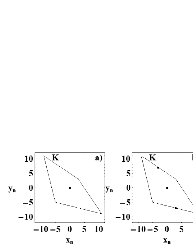
Figure 3: State space ${\mathcal{K}}$ and equilibrium solutions of the iterated Prisoner’s Dilemma game. In a), all the players in the collectivity choose their strategies with equal probabilities. In b), we have three possible equilibrium states. In each subensemble game one player follows a deterministic strategy with memory length $m=1$, and the other chooses its pure strategies with equal probabilities. Depending on the adopted policy, we can have different equilibrium states. In c), all the players have chosen a deterministic strategy with memory length $m=1$, and the game can have seven equilibrium states.

Suppose now that both representative players $P$ and $Q$ adopt a policy with memory length $m=1$. Analysing the results of Table 2, the best payoff per move for both players is obtained when player $P$ and $Q$ play tit-for-tat and both choose the initial strategy ’0’. The best payoff per move is also obtained when one at least of the contenders chooses ’0’ and the other plays according the tit-for-tat policy. In the case of policies of memory length $m=1$, the tit-for-tit policy forces cooperation. If one of the player plays tit-for-tat and the other player chooses another strategy, tit-for-tit ensures that the payoffs per move of both players are equal and the second player is not able to increase its payoff per move. If both players choose a tit-for-tat policy, depending on the initial condition, we can have four different equilibrium states of the game, Table 2 and Fig. 1c). In this case, two of them are the strict and the bargain Nash solutions. If one of the players chooses always the strategy ’1’, it corresponds to the deterministic policy $f_{1,3}$, and the outcome of the game against a tit-for-tat corresponds to the Nash strict equilibrium of the game. The seven equilibrium solutions of the Prisoner’s game are plotted in Fig. 3c).

If $P$ has to choose a policy against a player $Q$ that plays its strategies with equal probabilities, by (4.15) and (2.5), the best policy for $P$ is the one that maximizes,

$${\bar{P}}_{m,n}=\left(3-12{n_{0}^{m,n}\over 2^{m+1}}\right)$$

Therefore, in the Prisoner’s Dilemma game, the best policy corresponds to $n_{0}^{m,n}=0$, which corresponds to the policy function $f_{m,2^{m}-1}$. In this case, we have, ${\bar{P}}_{m,2^{m}-1}=3$ and ${\bar{Q}}_{m,2^{m}-1}=-7$, Fig. 3b).

A more detailed analysis of Fig. 3, shows that Nash bargain solutions and Nash strict solutions only exist when both players have deterministic policies. In the sense of ensemble averages, Nash solutions are not equilibrium solutions of a game.

6.2 The Hawk-Dove game

The Hawk-Dove game has been introduced by Maynard-Smith and Price [17] as a game theoretical basic model to describe animal conflicts. They have assumed two pure strategies: Hawk (’0’) and Dove (’1’). A player chooses Hawk or ’0’ if he acts fiercely, and chooses Dove or ’1’ if he looks fierce and then retires. In the context of evolutionary biology, this game aims to explain the struggle for a territory whose payoff is related with the number of offsprings. The payoff matrix of the Hawk-Dove game is,

$$A=\left(\begin{array}[]{cc}{1\over 2}(r-c)&r\\ 0&{r\over 2}+\varepsilon\end{array}\right)$$

where $r$ represents the reproductive value and $c$ is the cost of injury. In this game the Hawk strategy is dominant, provided $c<r$ and $\varepsilon<r/2$. If $\varepsilon>0$ and $\varepsilon<r/2$, the Hawk-Dove game is also dilemmatic. Globally, the species has advantage if everybody acts Dove, which is the non-dominant strategy.

If all players choose their strategies with equal probability, by Theorem 3.1, the mean payoff per player and move is,

$${\bar{P}}={\bar{Q}}={1\over 2}(r-{1\over 4}c)+\varepsilon$$

If $c<4r+8\varepsilon$, ${\bar{P}}={\bar{Q}}>0$, the Hawk-Dove game shows advantage for the species. If $c\geq 4r+8\varepsilon$, the cost of injury is too high and globally the mean payoff per player and move is non-positive.

If the representative players of the game choose a generalized tit-for-tat policy with memory length $m=1$, and $c<r$, both players have a positive mean payoff per move. If the players choose not being the first to play Hawk, they both obtain the highest mean payoffs per move.

In the Hawk-Dove non-cooperative and symmetric game, the tit-for-tat policy or imitation of the adversary move implies a positive payoff for both players, provided the cost of injury is not too high ($c<4r+8\varepsilon$).

7 Conclusions

The dynamics of an iterated game is described by a one-to-many map defined on a state space, [14]. Within this framework, the concept of mixed strategy leads to the definition of the equilibrium solution of a game. This equilibrium solution is obtained as the limit of the iterates of a one-to-many map. In general, for a specific game, the equilibrium solutions associated to the set of all mixed strategies span the state space of the game. The concepts of strict Nash equilibrium and bargain solutions of a game are discussed within this framework.

In applications of game theory to economics, ethics, sociology, biology, physics, etc., it is sometimes easy to identify rules of behaviour and interactions between agents and to make guesses about payoffs. However, it is difficult to argue about the (infinite) memory of all the past choices of the players, and to insure that opponent players remain the same during all the iterated game. Therefore, the way of evaluating a game, or a policy depends on the context in which the game is considered.

In order to evaluate a game, we have introduced the concept of representative ensemble of a game. This technique has been applied to the global evaluation of a game, without any specific considerations about policies. In this evaluation, all the players make their choices of pure strategies with equal probabilities. In this case, we have shown that the mean payoffs per move of the players are the mean value of the entries of the payoff matrices of the game.

To evaluate a deterministic policy with a finite memory length, we have calculated the mean payoffs per move of the players, for the case where one of the players has a deterministic policy and the other player chooses its pure strategies with equal probabilities. In this case, there exists a class of deterministic policies that forces equality of the mean payoffs per move of the players. This class of policies is the class of generalized tit-for-tat policies. When a representative player has a generalized tit-for-tat policy, in the limit of the iterated game, the payoffs of both representative players are equal. If a player tries to increase its payoff by changing its strategy and the other player plays tit-for-tat, the change in the strategy can increase or decrease the payoffs, but the payoffs per move of both players remain equal. Generalized tit-for-tat or imitation strategies force equalitarian payoffs per move. In dilemmatic games, the generalized tit-for-tat policy together with the condition of not being the first to defect, leads to the highest possible mean payoffs per move for the players.

Acknowledgments: This work has been partially supported by the POCTI Project P/FIS/13161/1998, and by Fundação para a Ciência e a Tecnologia, under a plurianual funding grant.

References

[1] J. von Neumann and O. Morgenstern, Theory of Games and Economic Behavior, Princeton University Press, 1944.

[2] J. Maynard Smith, Evolution and the Theory of Games, Cambridge University Press, 1982.

[3] R. Axelrod, The evolution of cooperation, Basic Books, Harper Collins Pub., 1984.

[4] D. Fudenberg and J. Tirole, Game Theory, The MIT Press, Cambridge, Massachusetts, 1993.

[5] H. W. Kuhn (ed.), Classics in Game Theory, Princeton Uni. Press, 1997.

[6] F. Vega-Redondo, Evolution, Games and Economic Behaviour, Oxford Uni. Press, 1996.

[7] D. A. Meyer, Quantum strategies, Phys. Rev. Lett., 82 (1999) 1052-1055.

[8] C. A. Holt and A. E. Roth, The Nash equilibrium: A perspective, Proc. Natl. Acad. Sci. USA, 101 (2004) 3999-4002.

[9] P. D. Taylor and L. B. Jonker, Evolutionary stable strategies and game dynamics, Math. Biosciences, 40 (1978) 145-156.

[10] J. Hofbauer and K. Sigmund, Evolutionary Games and Population Dynamics, Cambridge Uni. Press, 1998.

[11] H. W. Kuhn , Lectures on Game Theory, Princeton Uni. Press, 2003.

[12] Mesterton-Gibbons, M., An introduction to Game-Theorethic Modelling, American Mathematical Society, Providence, RI, 2000.

[13] J. Nash, Equilibrium points in n-person games, Proc. Natl. Acad. Sci. USA, 36 (1950) 48-49.

[14] S. Smale, The prisoner’s dilemma and dynamical systems associated to non-cooperative games, Econometrica, 48 (1980) 1617-1634.

[15] R. Tolman, The Principles of Statistical Mechanics, Dover, New York, 1979.

[16] V. I. Arnold and A. Avez, Probl mes Ergodiques de la M canique Classique, Gauthier-Villars, Paris, 1967.

[17] J. Maynard Smith and G. Price, The logic of animal conflicts, Nature, 246 (1973) 15-18.