An Information-Theoretic Approach to Network Modularity

Abstract

Exploiting recent developments in information theory, we propose, illustrate, and validate a principled information-theoretic algorithm for module discovery and resulting measure of network modularity. This measure is an order parameter (a dimensionless number between $0$ and $1$). Comparison is made to other approaches to module-discovery and to quantifying network modularity using Monte Carlo generated Erdös-like modular networks. Finally, the Network Information Bottleneck (NIB) algorithm is applied to a number of real world networks, including the “social” network of coauthors at the APS March Meeting 2004.

I Introduction

A goal of modeling is to describe the system in terms of less complex degrees of freedom while retaining information deemed relevant Tishby et al. (1999). Approaches to complexity reduction for networks include characterizing the network in terms of simple statistics (such as degree distributions  Jeong et al. (2000) or clustering coefficients Watts and Strogatz (1998)), subgraphs over-represented relative to an assumed null model (see for example, Holland and Leinhardt (1976); Shen-Orr et al. (2002); Artzy-Randrup et al. (2004)), and communities (see for example, Newman and Girvan (2004)).

In the case of communities, networks are coarse-grained into clusters of nodes, or modules, where nodes belonging to one cluster are highly interconnected, yet have relatively few connections to nodes in other clusters. This type of network complexity reduction may be particularly promising as an approach to network analysis, since many naturally-occurring networks, including biological Hartwell et al. (1999) and sociological Newman and Girvan (2004); Wasserman et al. (1994) networks are thought to be modular. Clearer, quantitative understanding of these ideas would be valuable in finding reduced complexity descriptions of networks, in visualizing networks, and in revealing global design principles. Two current challenges facing the community regarding network modularity include (i) the ability to quantify to what extent a given network is “modular” and (ii) the ability to identify the modules of a given network.

With regard to quantifying modularity, to our knowledge no mathematical definition has yet been proposed for a measure of modularity that could compare networks regardless of size, origin, or choice of partitioning. In their recent book, Schlosser and Wagner Schlosser and Wagner (2004) write “a generally accepted definition of a module does not exist and different authors use the concept in quite different ways.” They proceed to warn of the “danger that modularity will degenerate into a fashionable but empty phrase unless its precise meaning is specified.” Some steps in this direction have been suggested by Newman’s “assortativity coefficient” Newman and Girvan (2003), which quantifies the level of assortative mixing in a network, and its unnormalized form, called “modularity” Newman and Girvan (2004). However, these measures quantify the quality of a particular partitioning of the network for a given number of modules, but are not a property of the network itself that could serve to compare networks of different origins.

As for module discovery, a range of techniques for identifying the modules in a network have been utilized with various success. In his review article, Newman Newman (2003) summarizes these efforts under the broad category of hierarchical clustering in which one poses a similarity metric between pairs of vertices. Hierarchical clustering can be agglomerative, where the most similar nodes are iteratively merged (e.g. Ravasz et al. (2002)) or divisive, where edges between the least similar nodes are iteratively removed (e.g. Newman and Girvan (2004)). By modifying traditional divisive approaches to focus on most “between” edges rather than least similar vertices, Newman and Girvan Newman and Girvan (2004) recently proposed a new class of divisive algorithms for finding modules. Various measures of “edge-betweenness” are defined to identify edges that lie between communities rather than within communities. By iteratively removing edges with highest betweenness one can break down the network into disconnected components which define the modules.

In this manuscript we take a markedly different approach. The problem of finding reduced descriptions of systems while retaining information deemed relevant has been well-studied in the learning theory community. In particular, the information bottleneck Tishby et al. (1999); Slonim. (2002) provides a unified and principled framework for complexity reduction. By applying the information bottleneck on probability distributions defined by graph diffusion, we propose a new, principled, information-theoretic algorithm to identify modules in networks. We demonstrate that the Network Information Bottleneck (NIB) algorithm outperforms the currently used technique of edge-betweenness (i) in correctly assigning nodes to modules and (ii) in determining the optimal number of existing modules. Moreover, the new method naturally defines a network modularity measure which can compare any two undirected networks to the extent to which the topology of each can be summarized by modules over all scales. Information-theoretic bounds constrain this measure to be between $0$ and $1$. Finally, we apply our method to a collaboration network derived from the APS March Meeting 2004 and the E. coli genetic regulatory network.

II The Information Bottleneck: A Review

Brief Tishby et al. (1999) and detailed Slonim. (2002) discussions of the information bottleneck can be found elsewhere; we here review only the most salient features. The fundamental quantity in information theory is Shannon entropy $H[p(x)]\equiv-\sum_{x}p(x)\log p(x)$ measuring lack of information (or disorder) in a random variable $X$, and uniquely (up to a constant) defined by three plausible axioms Shannon and Weaver (1949). Knowledge of a second random variable $Y$ decreases the entropy in $X$ on average by an amount

$$I(X,Y)\equiv H(X)-\langle H(X|Y)\rangle\equiv H[p(x)]-\sum_{y}p(y)H[p(x|y)]$$ (1)

called the mutual information Cover and Thomas (1990), the average information gained about $X$ by the knowledge of $Y$. Eq. (1) is equivalent to

$$I(X,Y)=\sum_{x}\sum_{y}p(x,y)\log\frac{p(x,y)}{p(x)p(y)}=\langle\log\frac{p(x,y)}{p(x)p(y)}\rangle$$ (2)

revealing its symmetry in $X$ and $Y$. The mutual information thus measures how much information one random variable tells about the other, and is the basis of the information bottleneck.

Clustering can generally be described as the problem of extracting a compressed description of some data that captures information deemed relevant or meaningful. For example, we might want to cluster protein sequences, expecting that the cluster assignments contain information about the fold of the proteins; or we might want to cluster words in documents, expecting that the clusters capture information about the topic in which the words appear. Tishby et al.’s Tishby et al. (1999) key insight into this problem is the inclusion in the clustering algorithm of another random variable, called the relevance variable, which describes the information to be preserved. In the case of protein sequences, the relevance variable might be the protein fold; in the case of clustering words over documents, the relevance variable might be the topic.

Let $x\in X$ be the input random variable (e.g., protein sequences in the set of all observed sequnces; or words in a given dictionary, in the two examples above), $y\in Y$ the relevance variable, and $z\in Z$ the cluster assignment random variable . The information bottleneck outputs a probabilistic cluster assignment function $p(z|x)$ equal to the probability to be in cluster $z$ for a given input $x$. The clustering minimizes the mutual information between $X$ and $Z$ (“maximally compressing the data set”), while constraining the possible loss in mutual information between $Z$ and $Y$ (“preserving relevant information”). In other words, one seeks to pass or squeeze the information that $X$ provides about $Y$ through the “bottleneck” formed by the compressed $Z$.

The simplicity of the model Z relative to that of the world X is quantified by the entropy reduction ${\cal S}[p(z|x)]\equiv H(X)-I(X,Z)=H(X,Z)-H(Z)>0$. The gain in simplicity, however, comes with a loss of fidelity in our description of the world, quantified by the error ${\cal E}\equiv I(X,Y)-I(X,Z)>0$, the loss in information about the world when described by a model Z instead of the primitive description X. The trade-off between the error and the simplicity can be expressed in terms of the functional

$${\cal F}[p(z|x)]={\cal E}-T{\cal S}={\cal F}_{0}-I(X,Z)+TI(X,Z)$$ (3)

in which the temperature T parameterizes the relative importance of simplicity over fidelity. The term ${\cal F}_{0}$ is independent of the cluster assignment $p(z|x)$. Since $p(y|x,z)=p(y|x)$, this is the only degree of freedom over which the free energy ${\cal F}$ is to be minimized. In the annealed ground state ($T\rightarrow 0$) each possible state of the world $x\in X$ is assigned with unit probability to one and only one state of the model $z\in Z$ (i.e., $p(z|x)\in\{0,1\}$, a limit called ”hard clustering”). If the cardinalities $|Z|$ and $|X|$ are equal, we arrive at the fully detailed, trivial solution where the clusters $Z$ simply copy the original $X$. A formal solution to the information bottleneck problem is given in Tishby et al. (1999) and yields the following three self-consistent equations (with $\beta=1/T$),

$$\left\{\begin{array}[]{ll}p(z|x)&=\frac{p(z)}{Z(\beta,x)}e^{-\beta D_{KL}[p(y|x)||p(y|z)]}\\ p(z)&=\sum_{x}p(z|x)p(x)\\ p(y|z)&=\frac{1}{p(z)}\sum_{x}p(y|x)p(z|x)p(x)\end{array}\right.$$ (4)

where $Z(\beta,x)$ is a normalization (partition) function and $D_{KL}[p||q]\equiv\sum_{x}p(x)\log\frac{p(x)}{q(x)}$ is the Kullback-Leibler divergence (also called the relative entropy). The first of these equations makes clear that as one anneals to ground state, where $T\rightarrow 0$ and $\beta\rightarrow\infty$, the only solution is the hard clustering ($p(x|z)\in\{0,1\}$) limit. These three equations naturally lend themselves to an iterative algorithm proposed in Tishby et al. (1999) which is provably convergent and finds a locally optimal solution.

While in many applications a “soft” clustering might be of interest, for clarity we only consider the hard case in this paper: each node is associated with one and only one module. We use two different algorithms to find approximate solutions to the information bottleneck problem. Both of them take a fixed $|Z|$ ($|Z|<|X|$) as input and output hard clustering assignments for every node.

The first algorithm (self-consistent NIB) uses $\beta$ as an annealing parameter that starts at low values and increases step by step. At every given $\beta$ the locally optimal solution is computed by iterating over Equations (4). The solution for given $\beta$ is then taken as a starting point for the iterations with the next $\beta$. The second algorithm (agglomerative NIB) uses an agglomerative approach Slonim et al. (2000). At every step a pair of nodes is merged into a single node, where the pair is chosen such as to maximize the relevant information $I(Y,Z)$. It thus reduces $|Z|$ by one at every step, and stops when the desired $|Z|$ is reached.

III Diffusive Distributions Defined over Graphs

We wish to find a representation of a network in which groups of nodes have been represented by effective nodes; we argue that a modular description of the network is most successful when relevant information about the network is preserved. Posed in this language, it is clear that the act of finding modules in a network is a type of clustering, and the appropriate clustering framework is one that preserves the information deemed relevant.

Formulation of graph clustering in terms of the information bottleneck requires a joint distribution $p(y,x)$ to be defined on the graph, where $x$ designates nodes and $y$ designates a relevance variable. An appropriate distribution that captures structural information about the network is the one defined by graph diffusion. The relevance random variable $y$ then ranges over the nodes, as does $x$, and is defined by the node at which a random walker stands at a given time $t$ if the random walker was standing at node $x$ at time $0$. The conditional probability distribution $G_{ij}^{t}\equiv p^{t}(y_{i}|x_{j})$ is a Green’s function describing propagation from node $j$ to node $i$. For discrete time diffusion one can easily derive Chung (1997)

$$G^{t}=[WT^{-1}]^{t}\;\;\mbox{, ($t\in\mathbb{N}$)}$$ (5)

where $W$ is a symmetric weighted affitiny matrix of positive entries and $T_{ij}\equiv\delta_{ij}\sum_{l}W_{il}\equiv\delta_{ij}k_{i}$. For a graph, with identically-weighted edges, $k_{i}$ is the conventional degree (the number of neighbors of node $i$), and $W$ is the adjacency matrix ($W_{ij}=1$ iff $i$ is adjacent to $j$). Note that we here only consider connected graphs and, as defined, this approach treats directed and undirected graphs identically.

In the continuous time limit

$$G^{t}=e^{(WT^{-1}-1)t}=e^{-LT^{-1}t}\;\;\mbox{, ($t>0$)}$$ (6)

where we defined $L\equiv T-W$, the graph Laplacian Merris (1994). In the machine learning literature a “graph kernel” Kondor and Lafferty (2002) has been defined as

$$G^{t}=e^{-Lt}.$$ (7)

to learn from structured data. It corresponds to a probability distribution associated with a different diffusion rule assuming a degree-dependent permeability at every node. For comparison, we consider both of these joint distributions as possible input to the information bottleneck algorithm.

The characteristic time scale $\tau$ of the system is given by the inverse of the smallest non-zero eigenvalue of the diffusion operator exponent ($LT^{-1}$ or $L$ ). This time reflects the finite system size and characterizes large-scale behaviors. For example, in one dimension on a bounded domain of size $\ell$, the smallest non-zero eigenvalue of the Laplacian with diffusion constant $D$ is $\pi^{2}D/\ell^{2}$. For our algorithm we will thus choose $t=\tau$.

To calculate the joint probability distribution $p(y,x)=p(y|x)p(x)$ from the conditional probability distribution $G^{\tau}=p(y|x)$, we must specify a prior $p(x)$: the distribution of random walkers at time 0. Natural definitions include (i) a flat prior $p(x)={1}/{N}$, $N$ being the total number of nodes and (ii) a prior corresponding to the steady state distribution associated with the diffusion operator: $p(x)={1}/{N}$ or $p(x)=k_{x}/{\sum_{x}k_{x}}$, for $G^{\tau}=e^{-L\tau}$ or $G^{\tau}=e^{-LT^{-1}\tau}$, respectively, where $k_{x}$ is the degree of node $x$.

IV Quantifying Modularity

IV.1 Partition modularity – quality of a partitioning

Newman and Girvan  Newman and Girvan (2004) propose a modularity, a “measure of a particular division of a network”, as $Q=\sum_{i}[e_{ii}-(\sum_{j}e_{ij})(\sum_{k}e_{ik})]$, where $e_{ij}$ is the fraction of all edges connecting module $i$ and module $j$. It can be interpreted as the difference between the fraction of within-module edges and the expected fraction of within-module edges in an ensemble of networks created by randomizing all connections while holding constant the number of edges emanating from each module. $Q$ should therefore go to $0$ for randomly connected networks, and tend to $1-1/|Z|$ for a perfectly modular network with $|Z|$ equally sized modules. We herein refer to the measure $Q$ as partition modularity to distinguish it from network modularity which we define below based on information-theoretic quantities. Newman et al. also study the number of modules $|Z|_{\rm max}$ which maximizes $Q$ given a particular module discovery algorithm.

IV.2 Network modularity – summarizability of network structure

We here propose a new modularity measure $M$, a property of a given network rather than of a given partitioning, which quantifies the extent to which a network can be summarized in terms of modules.

Every clustering solution $p(z|x)$ determines an normalized “input information” $0<I(Z,X)/H(X)<1$ between input variable $X$ and cluster assignment $Z$, and an “output information” $0<I(Z,Y)/I(X,Y)<1$ between cluster assignment and relevance variable $Y$. The information curve is then plotted as ${I(Z,Y)}/{I(X,Y)}$ vs. ${I(Z,X)}/{H(X)}$ for every solution of Equation (4) for every possible number of clusters Tishby et al. (1999). An example is shown in Figure 3. The curve traced by minimizers of the functional Eqn. 3, which will not necessarily be computed by such approximating schemes as the AIB, is provably convave. For perfectly random data, which cannot be summarized, this curve lies along the diagonal $y=x$. Consistent with these observations, we find that synthetic graphs with high connectivity within defined modules, and low connectivity between different modules exhibit larger area under the information curve (data not shown). We thus define a new measure of network modularity: the area under the information curve. In the soft clustering case the information curve is continuous since solutions vary with every choice of $\beta\in[0,\infty)$. In the hard clustering case, which we study here, the information curve is only defined at discrete points corresponding to solutions for every possible number of clusters $|Z|$. The area can then be calculated by linear interpolation. Information-theoretic bounds constrain the range of $M$ allowing comparison of networks of varying number of nodes and edges, and is a property of the network itself, rather than a given partitioning.

V Tests on synthetic networks

V.1 Accuracy of the partitioning

We here test how well various NIB implementations with different diffusion operators can reconstruct modules in a network generated with a known modular structure. We also compare our method to the “edge-betweenness” algorithm recently proposed in Newman and Girvan (2004) for the same purpose of finding modules or “communities”. In Newman and Girvan (2004) the network is broken down into isolated components by iteratively removing edges with highest “betweenness” (several definitions of edge-betweenness are tested in Newman and Girvan (2004); we here use the “shortest path” betweenness, which was shown in Newman and Girvan (2004) to perform optimally).

As in Newman and Girvan (2004), we generate synthetic Erdös-like graphs via Monte Carlo with 128 nodes each and average degree 8 (average total of 512 edges). We also demand that the graphs be connected by rejecting generated graphs that have disconnected components. We impose a structure of 4 modules with 32 nodes each by introducing two different probabilities: $p_{\rm in}$ for edges inside modules and $p_{\rm out}$ for edges between different modules. The level of noise in the graph is thus controlled by $p_{\rm out}$. The higher $p_{\rm out}$, the harder it will be to recover the different modules. We first generate networks with $p_{\rm out}=0$ and then increase $p_{\rm out}$ while adjusting $p_{\rm in}$ such that the average degree remains fixed. When $p_{\rm in}=p_{\rm out}$, all modular structure is lost and we obtain a usual Erdös graph. We measure the accuracy of a proposed partitioning using the following computation. In principle any module proposed by the algorithm could match any “true” module with an associated error. We therefore try every possible permutation of the 4 proposed modules matching the 4 “true” modules, and consider the one permutation with the smallest total number of incorrectly assigned nodes. We define accuracy as the total fraction of correctly assigned nodes.

Figure 1a shows the accuracy of the recovered modules as a function of ${p_{\rm out}}/{p_{\rm in}}$ for three different algorithms: self-consistent NIB, agglomerative NIB, and betweenness. Both NIB algorithms use the physical diffusion operator $e^{-LT^{-1}t}$ and a flat prior $1/N$ to define a joint probability distribution. We observe that both NIB algorithms are much more successful in recovering the modular structure than the betweenness algorithm. A threshold noise level is achieved at around ${p_{\rm out}}/{p_{\rm in}}\approx 1/3$ for the NIB algorithms, and around ${p_{\rm out}}/{p_{\rm in}}\approx 1/6$ for the betweenness algorithm. The figure also shows that the self-consistent NIB in general finds a better partitioning than the agglomerative NIB.

Figure 1b shows the same measurements for self-consistent NIB algorithms using different diffusion operators as explained in Section III. For comparison the betweenness results are also plotted. Physical diffusion, defined by the continuous time limit, with an initial state $p(x)$ given by the equilibrium distribution $p(x)\propto k_{x}$, gives best performance.

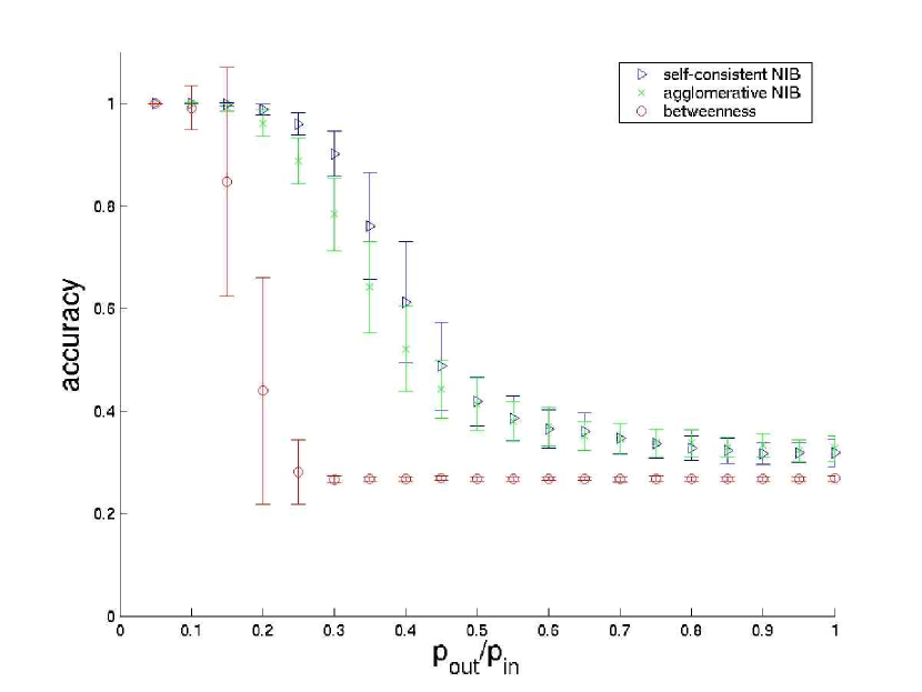
(a)

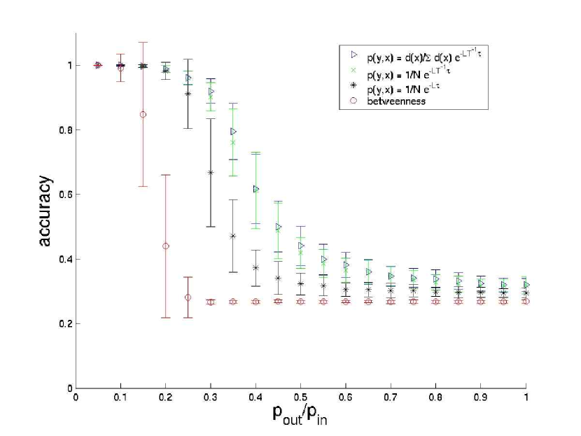
(b)

Figure 1: (a) Accuracy for different algorithms. Measured is the accuracy of recovering modular structure in syntheticnetworks under varying noise levels. Every point represents an average over 100 networks, each with 128 nodes and an average degree of 8. Both NIB algorithms outperform the betweenness algorithm.
(b) Accuracy for different diffusion operators Accuracy is measured in the same way as in (a), now using the self-consistent NIB algorithm with various diffusion operators to define probability distributions $p(y,x)$ over nodes. For comparison the betweenness results are also shown. The operator for physical diffusion $e^{-LT^{-1}t}$ outperforms the “graph kernel” diffusion operator proposed in the machine learning literature Kondor and Lafferty (2002).

V.2 Finding the optimal number of modules

In most real world problems the correct number of modules $|Z|$ present in the network is unknown a priori. It is therefore important to have an algorithm which not only computes a good partitioning for a given $|Z|$ but also gives a good estimate for $|Z|$ itself. To this end, we here make use of the partition modularity $Q$ as described in Section IV.1.

We again consider synthetic connected networks of 128 nodes and average degree 8 as in the previous section. However, we fix the noise level to a value of ${p_{\rm out}}/{p_{\rm in}}=0.3$ which was shown to be a critical level for these networks. We run the self-consistent NIB and the betweenness algorithms for every possible number of modules $|Z|=1,2,\dots,128$ and compute $Q$ for the proposed partitionings. Figure 2a shows $Q$ as a function of $|Z|$ for a typical run. While for the NIB algorithm $Q$ sharply peaks at the correct value of $|Z|_{\rm max}=4$, $Q$ calculated by the betweenness algorithm attains its maximum at $|Z|_{\rm max}=46$ and does not show a particular signal at $|Z|=4$. Figure 2b shows a histogram of $|Z|_{\rm max}$ for 100 generated networks. The NIB algorithm successfully identifies $|Z|_{\rm max}=4$ for 82% of the networks, while the betweenness algorithm calculates $|Z|_{\rm max}$ lying between $18$ and $89$, notably far from the correct value for any network. These experiments suggest that the NIB algorithm performs well both in accurately assigning nodes to modules and in revealing the optimal scale for partitioning.

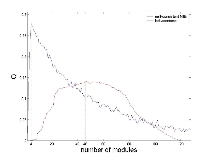
(a)

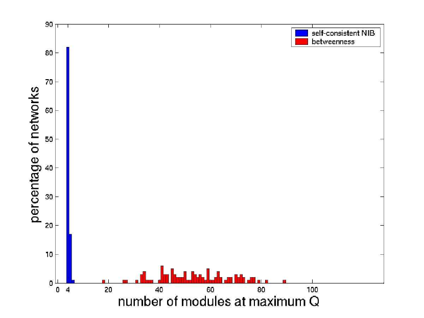
(b)

Figure 2: (a) $\mathbf{Q}$ vs. $\mathbf{|Z|}$. The quality of the partitioning $Q$ is computed for the partitionings output by the self-consistent NIB algorithm (with physical diffusion operator), and the betweenness algorithm, for every given number of modules $|Z|$. While the NIB algorithm correctly determines $|Z|=4$ as the best number of modules (at maximum $Q$), $Q$ calculated by the betweenness algorithm peaks at $|Z|=46$.
(b) Histogram of $|Z|_{\rm max}$ for 100 different networks. For 82% of the networks, the NIB algorithm is able to find the correct number of modules $|Z|_{\rm max}=4$, and comes close to it ($|Z|_{\rm max}=5$ or $6$) in all other cases. The betweenness algorithm gives $|Z|_{\rm max}$ between $18$ and $89$, far from the correct value for all networks.

VI Applications

VI.1 Collaboration Network

Having validated NIB on a toy model of modular networks, we next apply our algorithm to two examples of naturally-occurring networks. In the first example, we construct a collaboration network from the 2004 APS March Meeting, where this algorithm was first presented, and in the second example we construct a symmetric version of the E. coli genetic regulatory network.

Vertices of the collaboration network represent authors from all talks at the March Meeting; edges represent coauthorship. The largest component of the resulting graph consists of $5603$ vertices with $19761$ edges. Network information bottleneck using the agglomerative algorithm and the physical diffusion operator (as defined in Section III with its corresponding equilibrium distribution) reveals that this large network is highly modular ($m=0.9775$, see Figure 3a). For comparison, we also show the information curve for a typical Erdös network, which is clearly less modular. Such a high value of modularity implies that the authors of this component of the network are “easily” compressed or combined into larger clusters of authors. In the light of this fact, we study what the clusters of authors reveal about the collaboration network. For example, authors may group themselves according to topics or subject matters of the talks; alternatively, author modules may be more indicative of the authors’ affiliations or even geographical location.

To begin to approach these types of questions we may choose to look at the author groupings given by NIB at a particular number of clusters. While we emphasize that network modularity is a measure over all scales or all numbers of clusters, it is illustrative in this case also to examine the clustering at a particular scale. For the APS network, such an analysis yields the optimal number of modules, $|Z|_{\rm max}=115$, for this network (see Figure 3a).

In Figure 4 we plot the $115$ modules and their connections where each ellipse represents one module and edges between ellipses represent inter-modular connections. The sizes of the ellipses and the thickness of the edges are proportional to the log of the number of authors in a module and the log of the number of inter-modular connections between modules, respectively. We note the provocative structure revealed in the figure with a large center of highly connected modules (including two of the largest modules), three more or less branching, linear chains of modules, and one large $18$-node cycle of modules.

Closer inspection of a single module demonstrates that for many of the modules, institutional affiliation, and even geography, play a large role in determining collaborations. In Figure 5 a single $17$-node module is plotted where each node now represents an author and edges represent author collaborations. We see that $15$ of the $17$ authors are affiliated with Columbia University; the remaining two authors are affiliated with Stony Brook, and notably, are adjacent (indicating coauthorship) to each other. The finding that the modules in this collaboration network are somewhat related to institutional affiliations and geography is supported by similar results found in other physics collaboration networks previously studied using different techniques Newman and Girvan (2004).

Another possible annotation for this module to consider is that of the APS divisions and topical groups, since each author is associated with at least one talk and each talk is listed under one or more of these APS categories. However, the $14$ APS divisions and $10$ topical groups appear to be too broad and have too much overlap to clearly define a module. For example, the Columbia University module includes talks under the categories of Polymer, Condensed Matter, Material, and Chemical Physics. On the other hand, the module is essentially representative of researchers at the Columbia University Materials Research Science and Engineering Center (MRSEC) and in particular those interested in the synthesis of complex metal oxide nanocrystals. There is thus both topical and institutional information retained in the modules.

It is also revealing to examine the affiliations of multiple connected modules. For example, Figure 6 plots the uppermost branching linear chain of Figure 4. Here, color denotes module assignment as given by NIB. Most of these modules also have clear institutional affiliations. For example, everyone in the cyan module is at the Center of Complex Systems Research (CCSR) in Illinois; close to $80\%$ of the large green module is in China, mostly at the Institute of Chemistry Chinese Academy of Sciences (ICCAS); and $70\%$ of the red module is in England. The blue module is slightly more diffuse, though an institutional affiliation is also apparent here; over $50\%$ of the authors are affiliated with one of three institutions near Chicago (Argonne National Labs, University of Illinois at Chicago, and University of Notre Dame). The yellow and magenta modules are also overwhelmingly associated with the University of Nebraska, though interestingly our algorithm separates these two modules at this partitioning. In general, one does not anticipate that the optimal number of clusters in a given network will give the most natural partitioning at all scales and over all resulting modules.

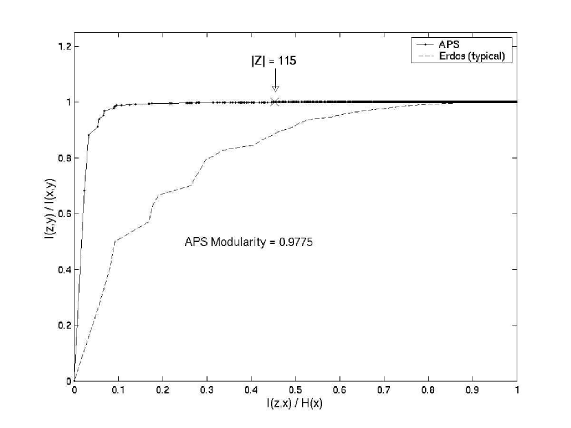
(a)

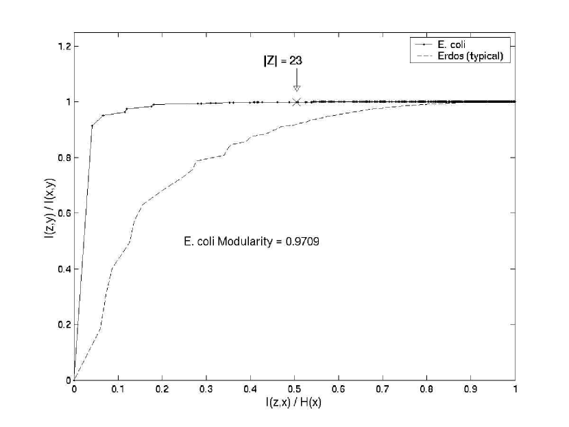
(b)

Figure 3: (a) APS Network Modularity. Information plane for the collaboration network obtained from the 2004 APS March Meeting (largest component consists of $5603$ authors and $19761$ edges). We use the agglomerative algorithm with the diffusion operator $e^{-LT^{-1}t}$. Network modularity for this graph, defined as the area under the curve is $0.9775$. Comparison is made with a typical information curve obtained from an Erdös graph. The optimal number of modules as defined by the the Newman and Girvan measure is at $|Z|=115$.
(b) E. coli Network Modularity. Information plane for the E. coli genetic regulatory network (largest component $328$ nodes and $456$ edges). We use the agglomerative algorithm with the diffusion operator $e^{-LT^{-1}t}$. Network modularity for this graph, defined as the area under the curve is $0.9709$. Comparison is made with a typical information curve obtained from an Erdös graph. The optimal number of modules as defined by the the Newman and Girvan measure is at $|Z|=23$.

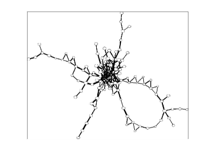
Figure 4: Adjacency network of the $115$ modules of the APS network. Nodes represent modules where the size of the drawn ellipse is proportional to the number of authors in the module. Edges between modules represent collaborations between authors in different modules, where the thickness of the drawn lines is proportional to the number of these inter-module collaborations. The module-network reveals a structure with highly dense center of modules, three branching linear chains of modules, and one cycle of modules.

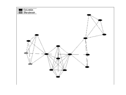
Figure 5: One of the $115$ modules of the APS network. Nodes represent authors and edges represent collaborations. Of the $17$ authors in the module, $15$ are Columbia-University affiliated and two are affiliated with Stony Brook University.

VI.2 Biological Network

The notion of modularity has been central in the study of a variety of biological networks including metabolic Ravasz et al. (2002), protein Maslov and Sneppen (2002); Han et al. (2004), and genetic Hartwell et al. (1999); Shen-Orr et al. (2002) networks. Certainly most biologists agree that the various networks operating within and between cells have a modular structure, though what they mean by “modular” can vary greatly Schlosser and Wagner (2004).

NIB allows us to investigate quantitatively and in detail to what extent naturally-occurring biological networks are modular. For example, Figure 7 depicts the undirected form of the largest component of the E. coli genetic regulatory network described previously in Shen-Orr et al. (2002) and Salgado et al. (2001). The network consists of $328$ vertices and $456$ edges and its modularity is depicted by the curve one traces in the information plane as the network is clustered using the network information bottleneck (see Figure 3b).

To establish whether the modularity of the network should be considered low, high, or moderate, we employ an ansatz popular in several reserach communities in which a distribution of networks is created by holding the in-, out-, and self-degree of each node constant but randomizing the connectivity of the graph, changing which nodes are connected to which neighbors Shen-Orr et al. (2002); Maslov and Sneppen (2002); Ziv et al. ; Holland and Leinhardt (1976); Snijders (1991); Connor and Simberloff (1979). The randomization, a variant of the configuration model Newman (2003), produces a distribution of networks from which we sample and then measure the network modularity. The histogram in Figure 8 shows that E. coli’s modularity is higher relative to this ensemble.

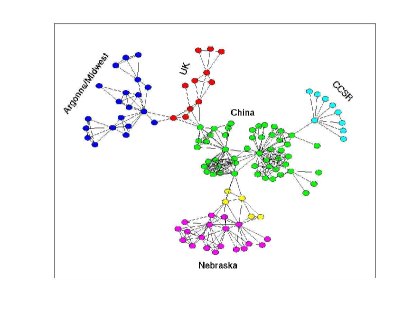
Figure 6: Six modules corresponding to the uppermost branched linear chain of modules depicted in Figure 4. Colors denote modules as defined by the network information bottleneck algorithm. Again the modules roughly correspond to institutional affiliations. Over $50\%$ of the blue nodes have one or more affiliations with the institutions based in and around Chicago (Argonne National Laboratory, University of Illinois at Chicago and University of Notre Dame). $70\%$ of the red nodes are in England, and $75\%$ of the green nodes are in China, mostly at the Institute of Chemistry Chinese Academy of Sciences, and all of the cyan nodes are at the Center of Complex Systems Research in Illinois. Both the yellow and magenta modules are mostly affiliated with the University of Nebraska.

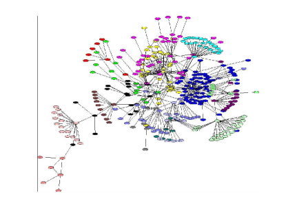
Figure 7: E. coli gene regulatory network. Largest component of the symmetric version of the E. coli genetic regulatory network. Colors denoted modules identified by NIB.

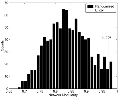
Figure 8: A histogram of network modularity, defined by the area underneath the curve in the information plane resulting from network compression, for $1000$ realizations of the variation of the configuration model. Note that the true E. coli network is more modular than the typical network resulting from the variation of the configuration model.

VII Conclusions and Extensions

We have presented a principled, quantitative, parameter-free, information-theoretic definition of network modularity, as well as an algorithm for discovering modules of a network. Network modularity is a dimensionless number between $0$ and $1$ and is a property of a given network over all scales, rather than of a given partitioning with a given number of modules. The measure is applicable to any network, including those with weighted edges. We validate the effectiveness of our algorithm in identifying the correct modules and in finding the true number of modules on synthetic, Monte Carlo generated, Erdös-like, modular networks. Finally, application to two real-world networks, a “social” network of physics collaborations and a biological network of gene interactions, is demonstrated.

Network modularity, the area under the curve in the information plane, is but one relevant statistic that we may retrieve from the information curve. Certainly other useful statistics may be culled. For example, the optimal information curve will always be concave Slonim. (2002) and its slope will decrease monotonically. The point at which the slope equals $1$ is uniquely determined for each network and can be described as the point after which clustering further results in a greater loss in relative relevant information than gain in relative compression (that is, $\delta\frac{I(Z,Y)}{I(X,Y)}=\delta\frac{I(Z,X)}{H(X)}$). This break-even point is the point at which one can gain further (normalized) simplicity only by losing an equivalent (normalized) fidelity. Numerical experiments and investigating the utility of this measure are currently in progress.

Diffusive distributions are but one general class of distributions on a network. A natural generalization of these ideas is to describe other distributions on a network for which a particular function, energy, or origin is known, and on which some particular degree of freedom (such as chemical concentration or genetic expression as a function of time) may be defined.

Finally, we note that while the information bottleneck is a prescription for finding the highest-fidelity summary of a system at a given simplicity, algorithms for determining network community structure are usually motivated by various definitions of normalized min-cuts Weiss (1999); Shi and Malik (Proc of IEEE Conf. on Comp. Vision and Pattern Recognition); Ng et al. (2001); Bach and Jordan (2004). Our results, particularly for the synthetic graphs with prescribed modular structure, demonstrate that information modularity implies edge modularity, an unexpected finding which motivates further numerical and analytic investigations in progress regarding this relationship.

Acknowledgments

It is a pleasure to acknowledge Mark Newman, Noam Slonim, Christina Leslie, Risi Kondor, Ilya Nemenman, and Susanne Still for many useful conversations on the information bottleneck and modularity. This work was supported by NSF ECS-0425850, NSF DMS-9810750, and NIH GM036277.

References

- Tishby et al. [1999] N. Tishby, F. Pereira, and W. Bialek, in Proceedings of the 37th Annual Allerton Conference on Communication, Control and Computing (University of Illinois Press, 1999), pp. 368–377, URL arxiv.org/abs/physics/0004057.
- Jeong et al. [2000] H. Jeong, B. Tombor, R.Albert, Z. Oltavi, and A.-L. Barabasi, Nature 407, 651 (2000).
- Watts and Strogatz [1998] D. J. Watts and S. H. Strogatz, Nature 393, 440 (1998).
- Shen-Orr et al. [2002] S. Shen-Orr, R. Milo, S. Mangan, and U. Alon, Nature Genetics 31 (2002).
- Holland and Leinhardt [1976] P. Holland and S. Leinhardt, Sociologic Methodology 7, 1 (1976).
- Artzy-Randrup et al. [2004] Y. Artzy-Randrup, S. J. Fleishman, N. Ben-Tal, and L. Stone, Science 305, 1107c (2004).
- Newman and Girvan [2004] M. Newman and M. Girvan, Phys. Rev. E 69, 026113 (2004).
- Hartwell et al. [1999] L. H. Hartwell, J. J. Hopfield, S. Leibler, and A. W. Murray, Nature 402, C47 (1999).
- Wasserman et al. [1994] S. Wasserman, K. Faust, and M. Granovetter, Social Network Analysis (Cambridge University Press, 1994).
- Schlosser and Wagner [2004] G. Schlosser and G. P. Wagner, Modularity in Development and Evolution (University of Chicago Press, 2004).
- Newman and Girvan [2003] M. Newman and M. Girvan, Phys. Rev. E 67, 026126 (2003).
- Newman [2003] M. Newman, SIAM Review 45, 167 (2003).
- Ravasz et al. [2002] E. Ravasz, A. Somera, D. Mongru, Z. Oltavi, and A.-L. Barabasi, Science 297, 1551 (2002).
- Slonim. [2002] N. Slonim., The information bottleneck: Theory and applications (2002).
- Shannon and Weaver [1949] C. Shannon and W. Weaver, The Mathematical Theory of Communication (University of Illinois Press, Urbana, Illinois, 1949).
- Cover and Thomas [1990] T. Cover and J. Thomas, Elements of Information Theory (John Wiley, New York, 1990).
- Slonim et al. [2000] N. Slonim, N. Friedman, and N. Tishby, in Proc. of NIPS-12, 1999 (MIT Press, 2000), pp. 617–623.
- Chung [1997] F. R. K. Chung, Spectral Graph Theory, no. 92 in Regional Conference Series in Mathematics (American Mathematical Society, 1997).
- Merris [1994] R. Merris, Linear Algebra and its Applications 197,198, 143 (1994).
- Kondor and Lafferty [2002] R. I. Kondor and J. Lafferty, in Proceedings of the International Conference on Machine Learning (ICML) (2002).
- Maslov and Sneppen [2002] S. Maslov and K. Sneppen, Science 296, 910 (2002).
- Han et al. [2004] J.-D. J. Han, N. Bertlin, T. Hao, D. S. Goldberg, G. F. Berriz, L. V. Zhang, D. Dupuy, A. J. Walhout, M. E. Cusick, F. P. Roth, et al., Nature 430, 88 (2004).
- Salgado et al. [2001] H. Salgado, S. G.-C. A. Santos-Zavaleta, D. Millan-Zarate, E. Diaz-Peredo, F. Sanchez-Solano, E. Perez-Rueda, C. Bonavides-Martinez, and J. Collado-Vides, Nucleic Acids Research 29, 72 (2001).
- [24] E. Ziv, R. Koytcheff, and C. H. Wiggins, Novel systematic discovery of statistically significant network features, submitted, eprint cond-mat/0306610.
- Connor and Simberloff [1979] E. F. Connor and D. Simberloff, Ecology 60, 1132 (1979).
- Snijders [1991] T. Snijders, Psychometrika 56, 397 (1991).
- Ng et al. [2001] A. Ng, M. Jordan, and Y. Weiss, Advances in Neural Information Processing Systems 14 (2001).
- Weiss [1999] Y. Weiss, Tech. Rep., CS Dept, UC Berkeley (1999).
- Shi and Malik [Proc of IEEE Conf. on Comp. Vision and Pattern Recognition] J. Shi and J. Malik (Proc of IEEE Conf. on Comp. Vision and Pattern Recognition).
- Bach and Jordan [2004] F. R. Bach and M. I. Jordan, in Advances in Neural Information Processing Systems 16, edited by S. Thrun, L. Saul, and B. Schölkopf (MIT Press, Cambridge, MA, 2004).