Signal processing of acoustic signals in the time domain with an active nonlinear nonlocal cochlear model

Abstract

A two space dimensional active nonlinear nonlocal cochlear model is formulated in the time domain to capture nonlinear hearing effects such as compression, multi-tone suppression and difference tones. The micromechanics of the basilar membrane (BM) are incorporated to model active cochlear properties. An active gain parameter is constructed in the form of a nonlinear nonlocal functional of BM displacement. The model is discretized with a boundary integral method and numerically solved using an iterative second order accurate finite difference scheme. A block matrix structure of the discrete system is exploited to simplify the numerics with no loss of accuracy. Model responses to multiple frequency stimuli are shown in agreement with hearing experiments. A nonlinear spectrum is computed from the model, and compared with FFT spectrum for noisy tonal inputs. The discretized model is efficient and accurate, and can serve as a useful auditory signal processing tool.

1 Introduction

Auditory signal processing based on phenomenological models of human perception has helped to advance the modern technology of audio compression [10]. It is of interest therefore to develop a systematic mathematical framework for sound signal processing based on models of the ear. The biomechanics of the inner ear (cochlea) lend itself well to mathematical formulation ([1, 2] among others). Such models can recover main aspects of the physiological data [13, 11] for simple acoustic inputs (e.g. single frequency tones). In this paper, we study a nonlinear nonlocal model and associated numerical method for processing complex signals (clicks and noise) in the time domain. We also obtain a new spectrum of sound signals with nonlinear hearing characteristics which can be of potential interest for applications such as speech recognition.

Linear frequency domain cochlear models have been around for a long time and studied extensively [8, 9]. The cochlea, however, is known to have nonlinear characteristics, such as compression, two-tone suppression and combination tones, which are all essential to capture interactions of multi-tone complexes [4, 5, 17]. In this nonlinear regime, it is more expedient to work in the time domain to resolve complex nonlinear frequency responses with sufficient accuracy. The nonlinearity in our model resides in the outer hair cells (OHC’s), which act as an amplifier to boost basilar membrane (BM) responses to low-level stimuli, so called active gain. It has been shown [3] that this type of nonlinearity is also nonlocal in nature, encouraging near neighbors on the BM to interact.

One space dimensional transmission line models with nonlocal nonlinearities have been studied previously for auditory signal processing [5, 16, 17, 15]. Higher dimensional models give sharper tuning curves and higher frequency selectivity. In section 2, we begin with a two space dimensional (2-D) macromechanical partial differential equation (PDE) model. We couple the 2-D model with the BM micromechanics of the active linear system in [9]. We then make the gain parameter nonlinear and nonlocal to complete the model setup, and do analysis to simplify the model.

In section 3, we discretize the system and formulate a second order accurate finite difference scheme so as to combine efficiency and accuracy. The matrix we need to invert at each time step has a time-independent part (passive) and a time-dependent part (active). In order to speed up computations, we split the matrix into the passive and active parts and devise an iterative scheme. We only need to invert the passive part once, thereby significantly speeding up computations. The structure of the system also allows us to reduce the complexity of the problem by a factor of two, giving even more computational efficiency. A proof of convergence of the iterative scheme is given in the Appendix.

In section 4, we discuss numerical results and show that our model successfully reproduces the nonlinear effects such as compression, multi-tone suppression, and combination difference tones. We demonstrate such effects by inputing various signals into the model, such as pure tones, clicks and noise. A nonlinear spectrum is computed from the model and compared with FFT spectrum for the acoustic input of a single tone plus Gaussian white noise. The conclusions are in section 5.

Figure 1: The figure on the left is a schematic of the cochlea, while the figure on the right represents the upper chamber with the macromechanical equations and boundary conditions.

2 Model Setup

2.1 Macromechanics

The cochlea consists of an upper and lower fluid filled chamber, the scala vestibuli and scala tympani, with a shared elastic boundary called the basilar membrane (BM) (see Figure 1). The BM acts like a Fourier transform with each location on the BM tuned to resonate at a particular frequency, ranging from high frequency at the basal end to low frequency at the apical end. The acoustic wave enters the ear canal, where it vibrates the eardrum and then is filtered through the middle ear, transducing the wave from air to fluid in the cochlea via the stapes footplate. A traveling wave of fluid moves from the base to the apex, creating a skew-symmetric motion of the BM. The pressure difference drives the BM, which resonates according to the frequency content of the passing wave.

We start with simplification of the upper cochlear chamber into a two dimensional rectangle $\Omega=[0,L]\times[0,H]$ (see Figure 1). Due to the symmetry, we can ignore the lower chamber. The bottom boundary ($z=0$) is the BM, while the left boundary ($x=0$) is the stapes footplate. The macromechanical equations are

$$\left\{\begin{array}[]{ll}\varDelta p(x,z,t)=\frac{\partial^{2}p}{\partial x^{2}}+\frac{\partial^{2}p}{\partial z^{2}}=0,\ x\in[0,L],\ z\in[0,H],\ t\in[0,\infty)\\ p_{x}(0,z,t)=T_{\mathrm{M}}p_{\mathrm{e}}(t),\ \ p(L,z,t)=0\\ p_{z}(x,0,t)=2\rho u_{tt},\ \ p_{z}(x,H,t)=0\end{array}\right.$$ (2.1)

where $p(x,z,t)$ is the pressure difference across the BM, $u(x,t)$ denotes BM displacement, and $\rho$ is fluid density.

At the stapes footplate $(0,z)$, $p_{\mathrm{e}}(t)$ is pressure at the eardrum while $T_{\mathrm{M}}$ is a bounded linear operator on the space of bounded continuous functions that incorporates the middle ear filtering characteristics. In the frequency domain, for each input $\e^{\mathrm{i}\omega t}$, $T_{\mathrm{M}}(\omega)=2\rho\mathrm{i}\omega/Z_{\mathrm{m}}$, where $Z_{\mathrm{m}}$ is the impedance of the middle ear. The middle ear amplification function is given by $a_{\mathrm{M}}=|T_{\mathrm{M}}|$. In our case, based on Guinan and Peake [7],

$$a_{\mathrm{M}}(f)=1.815f^{2}((1-\frac{f^{2}}{f_{\mathrm{m}}^{2}})^{2}+(2\zeta_{\mathrm{m}}f/f_{\mathrm{m}})^{2})^{-1/2},$$ (2.2)

where $f_{\mathrm{m}}=4\ \mathrm{kHz}$ is the middle ear characteristic frequency and $\zeta_{\mathrm{m}}=0.7$ is the middle ear damping ratio. Thus, for $p_{\mathrm{e}}(t)=A\exp\{2\pi\mathrm{i}f\}+c.c$, where c.c. is complex conjugate, we have $T_{\mathrm{M}}p_{\mathrm{e}}(t)=B\exp\{2\pi\mathrm{i}f\}+c.c.$, where $B=a_{\mathrm{M}}(f)A$.

For more complex stimuli, it is useful to model the middle ear in the time domain as a one-degree of freedom spring-mass system. The equivalent time domain formulation of the steady state middle ear is given by

$$\left\{\begin{array}[]{l}p_{\mathrm{e}}(t)=m_{\mathrm{m}}\ddot{s}(t)+c_{\mathrm{m}}\dot{s}(t)+k_{\mathrm{m}}s(t)\\ s(0)=\dot{s}(0)=0\end{array}\right.$$ (2.3)

where $s(t)$ is stapes displacement and $m_{\mathrm{m}}$, $c_{\mathrm{m}}$ and $k_{\mathrm{m}}$ are the mass, damping and stiffness of the middle ear. The stapes boundary condition in (2.1) is replaced by

$$p_{x}(0,z,t)=2\rho\ddot{s}(t)$$ (2.4)

One of the interesting effects of using the time domain middle ear model is that it reduces the dispersive instability in the cochlea (see [14]). It appears that the steady state middle ear model ignores important transient effects and phase shifts that help to reduce the shock to the cochlea.

At the helicotrema $(L,z)$, we have used the Dirichlet boundary condition $p(L,z,t)=0$. In [9], they used an absorbing boundary condition $p_{x}(L)=cp_{t}(L)$, where $c$ is a positive constant [9]. Other models use the Neumann condition $p_{x}(L)=0$. It has been stated that the frequency domain solutions are minimally affected by which boundary condition is chosen [8], and thus we have chosen the simpler Dirichlet condition. However, interesting results on choosing the best initial conditions to minimize transient effects (dispersive instability) has been shown in [14] using the Neumann condition. To summarize, the macromechanics consist of equations (2.1)–(2.4).

2.2 Micromechanics

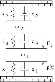
Figure 2: Cross section micromechanics of the cochlea. The mass $m_{1}$ represents a cross section of the BM, while mass $m_{2}$ is a cross section of the TM. (Reconstructed from Figure 3 in [9])

This is a resonant tectorial membrane model based on [9]. The BM and TM (tectorial membrane) are modeled as two lumped masses coupled by a spring and damper, with each mass connected to a wall by a spring and damper. (See Figure 2). A classical approximation is to have no longitudinal coupling except that which occurs through the fluid. Denoting $\xi(x,t)=(u(x,t),v(x,t))$ as BM and TM displacement, respectively, the equations of motion for the passive case at each point along the cochlea are given by

$$M_{\mathrm{p}}\ddot{\xi}+C_{\mathrm{p}}\dot{\xi}+K_{\mathrm{p}}\xi=F$$ (2.5)

where

$$M_{\mathrm{p}}=\left[\begin{array}[]{cc}m_{1}&0\\ 0&m_{2}\end{array}\right],\ \ C_{\mathrm{p}}=\left[\begin{array}[]{cc}c_{1}+c_{3}&-c_{3}\\ -c_{3}&c_{2}+c_{3}\end{array}\right],\ \ K_{\mathrm{p}}=\left[\begin{array}[]{cc}k_{1}+k_{3}&-k_{3}\\ -k_{3}&k_{2}+k_{3}\end{array}\right]$$ (2.6)

and forcing function

$$F=\left[\begin{array}[]{c}p(x,0,t)\\ 0\end{array}\right]$$ (2.7)

The parameters $m_{i}$, $c_{i}$, and $k_{i}$ are functions of $x$. The initial conditions are given by

$$\xi(x,0)=\dot{\xi}(x,0)=0$$ (2.8)

To make the model active, a self-excited vibrational force acting on the BM is added to (2.5):

$$M_{\mathrm{p}}\ddot{\xi}+C_{\mathrm{p}}\dot{\xi}+K_{\mathrm{p}}\xi=F+F_{\mathrm{a}}$$

where

$$F_{\mathrm{a}}=\left[\begin{array}[]{c}\gamma[c_{4}(\dot{u}-\dot{v})+k_{4}(u-v)]\\ 0\end{array}\right]$$

The difference $u-v$ represents OHC displacement. The parameter $\gamma\in[0,1]$ is the active gain control. In [9], this is a constant, but in our case will be a nonlinear nonlocal functional of BM displacement and BM location. Bringing $F_{\mathrm{a}}$ to the left, we have

$$M_{\mathrm{p}}\ddot{\xi}+(C_{\mathrm{p}}-\gamma C_{\mathrm{a}})\dot{\xi}+(K_{\mathrm{p}}-\gamma K_{\mathrm{a}})\xi=F$$ (2.9)

where

$$C_{\mathrm{a}}=\left[\begin{array}[]{cc}c_{4}&-c_{4}\\ 0&0\end{array}\right],\ \ K_{\mathrm{a}}=\left[\begin{array}[]{cc}k_{4}&-k_{4}\\ 0&0\end{array}\right]$$ (2.10)

Thus, the micromechanics consist of equations (2.6)–(2.10).

2.3 Nonlinear Nonlocal Active Gain

A compressive nonlinearity in the model is necessary to capture effects such as two-tone suppression and combination tones. Also, to allow for smoother BM profiles, we make the active gain nonlocal. Thus we have

$$\hat{u}(x,t)=\frac{2}{\sqrt{\lambda\pi}}\int_{0}^{L}\e^{-(x-s)^{2}/\lambda}u^{2}(s,t)\ \d s$$

and gain

$$\gamma(x,t)=\frac{1}{1+\theta\hat{u}}$$

where $\theta,\ \lambda$ are constants.

2.4 Semi-discrete Formulation

Solving the pressure Laplace equation on the rectangle using separation of variables, we arrive at

$$p(x,0,t)=T_{\mathrm{M}}p_{\mathrm{e}}(t)(x-L)+\sum_{n=1}^{\infty}A_{n}\cos\beta_{n}x$$ (2.11)

where

$$A_{n}=\left(\frac{-4\rho H}{L}\right)\left(\frac{\coth\beta_{n}H}{\beta_{n}H}\right)\int_{0}^{L}u_{tt}(x,t)\cos\beta_{n}x\d x$$ (2.12)

$$\beta_{n}=\frac{(n-\frac{1}{2})\pi}{L}$$

Substituting (2.11) into (2.7) and then discretizing (2.9) in space into $N$ grid points, we have

$$M\vec{\xi}_{tt}+C(t)\vec{\xi}_{t}+K(t)\vec{\xi}=\vec{b}(t)$$ (2.13)

where

$$M=\left[\begin{array}[]{cc}M_{1}+\alpha M_{\mathrm{f}}&0\\ 0&M_{2}\end{array}\right]$$

$$C(t)=C_{\mathrm{p}}-\hat{\Gamma}(t)C_{\mathrm{a}}=\left[\begin{array}[]{cc}C_{1}+C_{3}-\Gamma(t)C_{4}&-(C_{3}-\Gamma(t)C_{4})\\ -C_{3}&C_{2}+C_{3}\end{array}\right]$$

$$K(t)=K_{\mathrm{p}}-\hat{\Gamma}(t)K_{\mathrm{a}}=\left[\begin{array}[]{cc}K_{1}+K_{3}-\Gamma(t)K_{4}&-(K_{3}-\Gamma(t)K_{4})\\ -K_{3}&K_{2}+K_{3}\end{array}\right]$$

$$\vec{b}(t)=\left[\begin{array}[]{c}T_{\mathrm{M}}p_{\mathrm{e}}(t)(\vec{x}-L)\\ 0\end{array}\right]$$

$$M_{\mathrm{f},ij}=\sum_{k=1}^{K}\frac{\coth\beta_{k}H}{\beta_{k}H}\cos(\beta_{k}x_{i})\cos(\beta_{k}x_{j})w_{j}$$

$$\alpha=\frac{4\rho H}{N-1}$$

$C_{\mathrm{p}}$, $K_{\mathrm{p}}$, $C_{\mathrm{a}}$ and $K_{\mathrm{a}}$ are now block diagonal, where $K_{i}=\hbox{diag}\{k_{i}\}$ and $C_{i}=\hbox{diag}\{c_{i}\}$. Also, $M_{i}=\hbox{diag}\{m_{i}\}$, $\Gamma(t)=\hbox{diag}\{\gamma_{i}(t)\}$ and $\hat{\Gamma}(t)=\hbox{diag}\{\Gamma(t),0\}$. The numbers $w_{j}$ are numerical integration weights in the discretization of (2.12) and are chosen based on the desired degree of accuracy. Note that we can write $M_{\mathrm{f}}=M_{\mathrm{f}}^{\mathrm{s}}W$, where $W=\hbox{diag}(w_{j})$ and $M_{\mathrm{f}}^{\mathrm{s}}$ is symmetric and positive definite. The result of separation of variables produced the matrix $M_{\mathrm{f}}$, which is essentially the mass of fluid on the BM and dynamically couples the system.

3 Numerics

In formulating a numerical method, we note that the matrices in (2.13) can be split into a time-independent passive part and a time-dependent active part. In splitting in this way, we are able to formulate an iterative scheme where we only need to do one matrix inversion on the passive part for the entire simulation. Thus, using second order approximations of the first and second derivates in (2.13), we arrive at

$$(L_{\mathrm{p}}-L_{\mathrm{a}}^{n})\vec{\xi}^{n+1}=\vec{B}^{n}\;\;\;\Longrightarrow\;\;\;\vec{\xi}^{n+1,k+1}=L_{\mathrm{p}}^{-1}\vec{B}^{n}+L_{\mathrm{p}}^{-1}L_{\mathrm{a}}^{n}\vec{\xi}^{n+1,k}$$ (3.14)

where superscript $n$ denotes discrete time, $k$ denotes iteration and

$$L_{\mathrm{p}}=2M+\frac{3}{2}\Delta{t}C_{\mathrm{p}}+\Delta{t}^{2}K_{\mathrm{p}}$$

$$L_{\mathrm{a}}^{n}=\hat{\Gamma}^{n}[\frac{3}{2}\Delta{t}C_{\mathrm{a}}+\Delta{t}^{2}K_{\mathrm{a}}]$$

$$\vec{B}^{n}=\Delta{t}^{2}\vec{b}(n\Delta{t})+M(5\vec{\xi}^{n}-4\vec{\xi}^{n-1}+\vec{\xi}^{n-2})+\frac{\Delta{t}}{2}C^{n}(4\vec{\xi}^{n}-\vec{\xi}^{n-1}).$$

Proof of convergence will follow naturally from the next discussion. Notice that this is a $2N\times 2N$ system. We shall simplify it to an $N\times N$ system and increase the computational efficiency.

3.1 System Reduction

We write $L_{\mathrm{p}}$ and $L_{\mathrm{a}}^{n}$ in block matrix form as

$$L_{\mathrm{p}}=\left[\begin{array}[]{cc}\tilde{M}_{1}&-P_{3}\\ -P_{3}&\tilde{M}_{2}\end{array}\right]$$

$$L_{\mathrm{a}}^{n}=\left[\begin{array}[]{cc}\Gamma^{n}P_{4}&-\Gamma^{n}P_{4}\\ 0&0\end{array}\right]$$

where

$$\tilde{M}_{1}=2(\alpha M_{\mathrm{f}}+M_{1})+P_{1}+P_{3}$$

$$\tilde{M}_{2}=2M_{2}+P_{2}+P_{3}$$

$$P_{i}=\frac{3}{2}\Delta{t}C_{i}+\Delta{t}^{2}K_{i}$$

It is easily seen that the left inverse of $L_{\mathrm{p}}$ is given by

$$L_{\mathrm{p}}^{-1}=\left[\begin{array}[]{cc}D^{-1}&D^{-1}\tilde{M}_{2}^{-1}P_{3}\\ \tilde{M}_{2}^{-1}P_{3}D^{-1}&\tilde{M}_{2}^{-1}P_{3}D^{-1}\tilde{M}_{1}P_{3}^{-1}\end{array}\right]$$

where

$$D = \tilde{M}_{1}-P_{3}\tilde{M}_{2}^{-1}P_{3}$$ (3.15)

$$= 2\alpha M_{\mathrm{f}}+[2M_{1}+P_{1}+P_{3}(I-\tilde{M}_{2}^{-1}P_{3})]$$

$$= \{2\alpha M_{\mathrm{f}}^{\mathrm{s}}+[2M_{1}+P_{1}+P_{3}(I-\tilde{M}_{2}^{-1}P_{3})]W^{-1}\}W$$

$$\equiv D_{\mathrm{s}}W$$

Note that $D$ is invertible since $M_{\mathrm{f}}^{\mathrm{s}}$ is positive definite, thus invertible, and all other terms are positive diagonal matrices, and thus their sum is positive definite and invertible. We also have

$$L_{\mathrm{p}}^{-1}L_{\mathrm{a}}^{n}=\left[\begin{array}[]{cc}D^{-1}\Gamma^{n}P_{4}&-D^{-1}\Gamma^{n}P_{4}\\ \tilde{M}_{2}^{-1}P_{3}D^{-1}\Gamma^{n}P_{4}&-\tilde{M}_{2}^{-1}P_{3}D^{-1}\Gamma^{n}P_{4}\end{array}\right]$$ (3.16)

Letting $\vec{B}^{n}=(\vec{B}_{1}^{n},\vec{B}_{2}^{n})$, we have

$$\vec{u}^{n+1,k+1} = W^{-1}[\zeta_{1}^{n}+D_{\mathrm{s}}^{-1}\Gamma^{n}P_{4}(\vec{u}-\vec{v})^{n+1,k}]$$ (3.17)

$$\vec{v}^{n+1,k+1} = W^{-1}\tilde{M}_{2}^{-1}P_{3}[\zeta_{2}^{n}+D_{\mathrm{s}}^{-1}\Gamma^{n}P_{4}(\vec{u}-\vec{v})^{n+1,k}]$$ (3.18)

where

$$\zeta_{1}^{n}=D_{\mathrm{s}}^{-1}[\vec{B}_{1}^{n}+\tilde{M}_{2}^{-1}P_{3}\vec{B}_{2}^{n}]$$ (3.19)

$$\zeta_{2}^{n}=D_{\mathrm{s}}^{-1}[\vec{B}_{1}^{n}+\tilde{M}_{1}P_{3}^{-1}\vec{B}_{2}^{n}]$$ (3.20)

At each time step, we do 2 $N\times N$ matrix solves in (3.19) and (3.20) to initialize the iterative scheme. Then, since the same term appears in both equations (3.17) and (3.18), for each $k$ we only have to do 1 $N\times N$ matrix solve. In practice, since $D_{\mathrm{s}}$ is symmetric, positive definite and time-independent, we compute the Cholesky factorization of $D_{\mathrm{s}}$ at the start of the simulation and use the factorization for more efficient matrix solves at each step. As a side note, if we subtract (3.18) from (3.17), we have one equation for the OHC displacement $u-v$.

4 Numerical Results

4.1 Model Parameters

We start with a modification of the parameters in [9] (See Table 1). It is known that higher dimensional models give higher sensitivity. This is the case with this model. The 1-D model [9] gives a 90 dB active gain at 16 kHz, whereas the 2-D model gives a 160 dB active gain. Thus, we need to tune the system to reduce the gain. There are many ways to do this, and the method we choose is to increase all the damping coefficients in the table by the following:

$$2\e^{0.2773x}c_{i}\mapsto c_{i},\ \ i=1,2,3,4$$

Table 1: Model parameters in cgs units

$m_{1}(x)$	$3\cdot 10^{-3}\ \mathrm{g}\cdot\mathrm{cm}^{-2}$	$m_{\mathrm{m}}$	$34.4\cdot 10^{-3}\ \mathrm{g}\cdot\mathrm{cm}^{-2}$
$c_{1}(x)$	$20+1500\e^{-2x}\ \mathrm{dyn}\cdot\mathrm{s}\cdot\mathrm{cm}^{-3}$	$c_{\mathrm{m}}$	$1.21\cdot 10^{3}\ \mathrm{dyn}\cdot\mathrm{s}\cdot\mathrm{cm}^{-3}$
$k_{1}(x)$	$1.1\cdot 10^{9}\e^{-4x}\ \mathrm{dyn}\cdot\mathrm{cm}^{-3}$	$k_{\mathrm{m}}$	$2.18\cdot 10^{7}\ \mathrm{dyn}\cdot\mathrm{cm}^{-3}$
$m_{2}(x)$	$0.5\cdot 10^{-3}\ \mathrm{g}\cdot\mathrm{cm}^{-2}$	$L$	$2.5$ cm
$c_{2}(x)$	$10\e^{-2.2x}\ \mathrm{dyn}\cdot\mathrm{s}\cdot\mathrm{cm}^{-3}$	$H$	$0.1$ cm
$k_{2}(x)$	$7\cdot 10^{6}\e^{-4.4x}\ \mathrm{dyn}\cdot\mathrm{cm}^{-3}$	$\rho$	$0.1\ \mathrm{g}\cdot\mathrm{cm}^{-3}$
$c_{3}(x)$	$2\e^{-0.8x}\ \mathrm{dyn}\cdot\mathrm{s}\cdot\mathrm{cm}^{-3}$	$\theta$	$0.5$
$k_{3}(x)$	$10^{7}\e^{-4x}\ \mathrm{dyn}\cdot\mathrm{cm}^{-3}$	$\lambda$	$0.08$ cm
$c_{4}(x)$	$1040\e^{-2x}\ \mathrm{dyn}\cdot\mathrm{s}\cdot\mathrm{cm}^{-3}$	$\Delta t$	$2.5\cdot 10^{-6}$ – $10^{-5}$ s
$k_{4}(x)$	$6.15\cdot 10^{8}\e^{-4x}\ \mathrm{dyn}\cdot\mathrm{cm}^{-3}$	$N$	$401$

4.2 Isointensity Curves

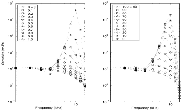
Figure 3: Both figures are sensitivity curves for CP = 0.77 cm or CF = 10 kHz. The left plot is a collection of sensitivity curves for the linear steady state active model where the parameter is the active gain $\gamma$. The right plot is a collection of sensitivity curves for the nonlinear time domain model where the parameter is pressure at the eardrum in dB SPL (sound pressure level).

In an isocontour plot, a probe is placed at a specific location on the BM where the time response is measured and analyzed for input tones covering a range of frequencies. Figure 3 shows isointensity curves for $\mathrm{CF}=10\ \mathrm{kHz}$, which corresponds to $\mathrm{CP}=0.77\ \mathrm{cm}$. The characteristic place (CP) for a frequency is defined as the location on the BM of maximal response from a pure tone of that frequency in the fully linear active model ($\gamma=1$). The characteristic frequency (CF) at a BM location is the inverse of this map. The left plot is the linear steady state active case. The parameter is the active gain $\gamma$, and for each value of the active gain we get a curve that is a function of the input frequency. The value of this function is the ratio $|u|(\mathrm{CP})/P_{\mathrm{e}}$, where $|u|(\mathrm{CP})$ is BM displacement at the characteristic place and $P_{\mathrm{e}}$ is pressure at the eardrum. This is known as sensitivity. It is basically an output/input ratio and gives the transfer characteristics of the ear at that particular active level. Notice that when $\gamma=1$, the BM at the characteristic place is most sensitive at the corresponding characteristic frequency, but at lower values of the gain, the sensitivity peak shifts to lower frequencies.

Analogously, the second plot in Figure 3 shows isointensity curves for the nonlinear time domain model where now the parameter is the intensity of the input stimulus in dB SPL (sound pressure level). For the time domain, we measure the root-mean-square BM amplitude from 5 ms (to remove transients) up to a certain time $T$. Note that for high-intensity tones, the model becomes passive while low-intensity tones give a more active model. This shows compression. Again, there is a frequency shift of the sensitivity peak (about one-half octave) from low to high-intensity stimuli in agreement with [11], so called half-octave shift. The plot agrees well with Figure 5 in [11].

4.3 Complex Stimuli

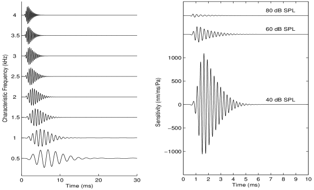
Figure 4: An impulse, or click, lasting 0.1 ms starting at 0.4 ms is input into the nonlinear nonlocal ear model. The left plot is the BM displacement time series for various CF’s ranging from 0.5-4 kHz. The right plot is a sensitivity plot for various stimulus intensities at CF = 6.4 kHz.

The first non-sinusoidal input we look at is a click. In the experiment in the left plot of Figure 4, we put probes at varying characteristic places associated with frequencies ranging from 0.5-4 kHz to measure the time series BM displacement. The click was 40 dB with duration 0.1 ms starting at 0.4 ms. All responses were normalized to amplitude 1. The plot is similar to Figure 4 in [5]. In the right plot of Figure 4, a probe was placed at CP for 6.4 kHz and the time series BM volume velocity was recorded for various intensities and the sensitivity plotted. This shows, similar to Figure 3, the compression effects at higher intensities. See Figure 9 in [11] for a similar plot.

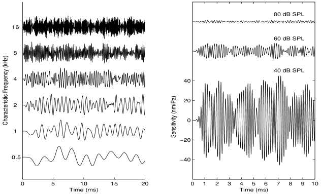
Figure 5: Gaussian noise is input into the ear. The left plot is the BM displacement times series for various CF’s ranging from 0.5-16 kHz. The right plot is a sensitivity plot for CF = 6.4 kHz.

The second non-sinusoidal input we explore is Gaussian white noise. Figure 5 is similar in all regards to Figure 4. Notice again in the right plot the compression effect.

4.4 Difference Tones

Figure 6: Two sinusoidal tones, 7 and 10 kHz at 80 dB each, are the input. The left and middle plots are snapshots at 15 ms of BM displacement and active gain, respectively. The right plot is a spectrum plot of the BM displacement time series at CP for 4 kHz.

Any nonlinear system with multiple sinusoidal inputs will create difference tones. If two frequencies $f_{1}$ and $f_{2}$ are put into the ear, $nf_{1}\pm mf_{2}$ will be created at varying intensities, where $n$ and $m$ are nonnegative integers. The cubic difference tone, denoted $f=2f_{1}-f_{2}$, where $f_{1}<f_{2}$, is the most prominent. Figure 6 contains three plots of one experiment. The experiment consists of two sinusoidal tones, 7 and 10 kHz at 80 dB each. The cubic difference tone is 4 kHz. The plot on the left is the BM profile for the experiment at 15 ms. We see combination tone peaks at 1.21 cm (CP for 4 kHz), 1.54 cm (CP for 2 kHz) and 1.85 cm (CP for 1 kHz). The middle plot shows the snapshot at 15 ms of the active gain parameter, showing the difference tones getting an active boost. Finally, the right plot is a spectrum plot of the time series for BM displacement at 1.21 cm, the characteristic place for 4 kHz. The cubic difference tone is above 1 nm and can therefore be heard.

4.5 Multi-tone Suppression

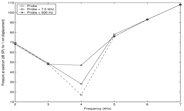
Figure 7: Isodisplacement curves at CP for 4 kHz showing responses to single tones (dashed line w/ circle) and responses to the same tones in the presence of high-side and low-side suppressors presented at 80 dB SPL.

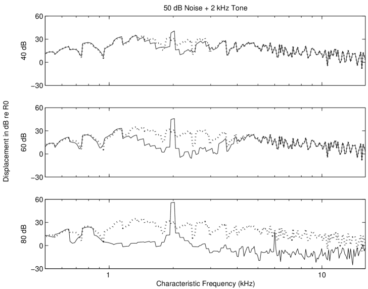
Figure 8: Spectrum plots of BM responses for characteristic frequencies along the BM, from 500 Hz to 16 kHz, with 50 dB noise and a 2 kHz tone ranging from 40-80 dB. R0 is the average of the BM response spectrum of 0 dB noise from 0.5-16 kHz. The solid line represents noise with tone, the dotted line noise without tone.

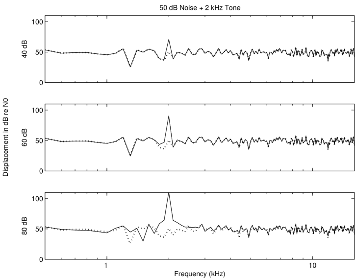
Figure 9: Spectrum plots of input signals consisting of 50 dB noise and a 2 kHz tone ranging from 40-80 dB. N0 is the average of the spectrum of 0 dB noise from 0.5-16 kHz. The solid line represents noise with tone, the dotted line noise without tone.

Two-tone (and multi-tone) suppression is characteristic of a compressive nonlinearity and has been recognized in the ear [11, 4, 6]. Figure 7 illustrates two-tone suppression and is a collection of isodisplacement curves that show decreased tuning in the presence of suppressors and is similar to Figure 16 in [11]. We placed a probe at the CP for 4 kHz (1.21 cm) and input sinusoids of various frequencies. At each frequency, we record the pressure at the eardrum that gives a 1 nm displacement for 4 kHz in the FFT spectrum of the time series response at CP. The curve without suppressors is dashed with circles. We then input each frequency again, but this time in the presence of a low side (0.5 kHz) tone and high side (7.5 kHz) tone, both at 80 dB. Notice the reduced tuning at the CF. Also notice the asymmetry of suppression, which shows low side is more suppressive than high side, in agreement with [6].

For multi-tone suppression, we look at tonal suppression of noise. In Figure 8, for each plot, a probe was placed at every grid point along the BM and the time response was measured from 15 ms up to 25 ms. The signal in each consisted of noise at 50 dB with a 2 kHz tone ranging from 40 dB to 80 dB (top to bottom). An FFT was performed for each response and its characteristic frequency amplitude was recorded and plotted in decibels relative to the average of the response spectrum of 0 dB noise from 0.5-16 kHz. We see suppression of all frequencies, with again low-side suppression stronger than high-side suppression. Figure 8 is qualitatively similar to Figure 3 in [4]. It is useful to compare this figure with Figure 9. This figure is the same as Figure 8, except we do an FFT of the input signal at the eardrum. Comparing these two figures shows that we have a new spectral transform that can be used in place of an FFT in certain applications, for example signal recognition and noise suppression.

5 Conclusions

We studied a two-dimensional nonlinear nonlocal variation of the linear active model in [9]. We then developed an efficient and accurate numerical method and used this method to explore nonlinear effects of multi-tone sinusoidal inputs, as well as clicks and noise. We showed numerical results illustrating compression, multi-tone suppression and difference tones. The model reached agreement with experiments [11] and produced a novel nonlinear spectrum. In future work, we will analyze the model responses to speech and resulting spectra for speech recognition. It is also interesting to study the inverse problem [12] of finding efficient and automated ways to tune the model to different physiological data. Applying the model to psychoacoustic signal processing [15] will be another fruitful line of inquiry.

Appendix A Appendix: Convergence of Iterative Scheme (3.14)

We need the following Lemma:

Lemma 1

If

$$M=\left[\begin{array}[]{cc}A&-A\\ B&-B\end{array}\right]$$

then every non-zero eigenvalue of $M$ is an eigenvalue of $A-B$.

[Proof.]

Let $\lambda$ be a non-zero eigenvalue of $M$ with non-trivial eigenvector $\vec{x}=(\vec{x}_{1},\vec{x}_{2})$. Thus, $M\vec{x}=\lambda\vec{x}$ gives

$$A(\vec{x}_{1}-\vec{x}_{2})=\lambda\vec{x}_{1}$$ (1.21)

$$B(\vec{x}_{1}-\vec{x}_{2})=\lambda\vec{x}_{2}$$ (1.22)

Subtracting the two equations, we have

$$(A-B)(\vec{x}_{1}-\vec{x}_{2})=\lambda(\vec{x}_{1}-\vec{x}_{2})$$

Now, if $\vec{x}_{1}-\vec{x}_{2}=0$, then from 1.21 and 1.22 above and $\lambda\neq 0$, we have $\vec{x}_{1}=\vec{x}_{2}=0$. But this means $\vec{x}=0$, which is a contradiction. Thus, $\lambda$ is an eigenvalue of $A-B$ with non-trivial eigenvector $\vec{x}_{1}-\vec{x}_{2}.$∎

Theorem 2

There exists a constant $C>0$ such that if $\Delta{t}<C$, then

$$\rho(L_{\mathrm{p}}^{-1}L_{\mathrm{a}}^{n})<1$$

where $\rho$ is the spectral radius. Thus, the iterative scheme converges.

[Proof.]

By the above lemma applied to (3.16), with constant $\gamma$, we have

$$\sigma(L_{\mathrm{p}}^{-1}L_{\mathrm{a}}^{n}) \subset \gamma\sigma(D^{-1}P_{4}-\tilde{M}_{2}^{-1}P_{3}D^{-1}P_{4})$$

$$= \gamma\sigma[(I-\tilde{M}_{2}^{-1}P_{3})D^{-1}P_{4}]$$

where $\sigma$ denotes spectrum. Thus, we have

$$\rho(L_{\mathrm{p}}^{-1}L_{\mathrm{a}}^{n}) \leq \gamma||(I-\tilde{M}_{2}^{-1}P_{3})W^{-1}D_{\mathrm{s}}^{-1}P_{4}||_{2}$$

$$\leq \gamma||(I-\tilde{M}_{2}^{-1}P_{3})W^{-1}||_{2}||D_{\mathrm{s}}^{-1}||_{2}||P_{4}||_{2}$$

Now, let $(\lambda,\vec{x})$ be the eigen-pair of $D_{\mathrm{s}}$ with $\lambda$ the smallest eigenvalue and $||\vec{x}||=1$. Note that $\lambda>0$ since $D_{\mathrm{s}}$ is positive definite. Thus, we have $1/\lambda$ is the largest eigenvalue of $D_{\mathrm{s}}^{-1}$, which gives

$$||D_{\mathrm{s}}^{-1}||_{2}\leq 1/\lambda$$

Thus, using the definition of $D_{\mathrm{s}}$ from (3.15), we have

$$\lambda = \vec{x}^{T}D_{\mathrm{s}}\vec{x}$$

$$= \vec{x}^{T}\{2\alpha M_{\mathrm{f}}^{\mathrm{s}}+[2M_{1}+P_{1}+P_{3}(I-\tilde{M}_{2}^{-1}P_{3})]W^{-1}\}\vec{x}$$

$$\geq \vec{x}^{T}\{[2M_{1}+P_{1}+P_{3}(I-\tilde{M}_{2}^{-1}P_{3})]W^{-1}\}\vec{x}$$

$$\geq \min\{[2m_{1}+p_{1}+p_{3}(1-\tilde{m}_{2}^{-1}p_{3})]w^{-1}\}$$

where lowercase represents diagonal entries. The third line above follows from $2\alpha M_{\mathrm{f}}^{\mathrm{s}}$ being positive definite. Finally, we have

$$\rho(L_{\mathrm{p}}^{-1}L_{\mathrm{a}}^{n}) \leq \gamma||(I-\tilde{M}_{2}^{-1}P_{3})W^{-1}||_{2}||D_{\mathrm{s}}^{-1}||_{2}||P_{4}||_{2}$$

$$\leq \gamma\frac{\max[(1-\tilde{m}_{2}^{-1}p_{3})w^{-1}]\max(p_{4})}{\min\{[2m_{1}+p_{1}+p_{3}(1-\tilde{m}_{2}^{-1}p_{3})]w^{-1}\}}$$

For $\Delta{t}$ small enough, we have convergence.∎

With our parameters, for convergence it is sufficient that $\Delta{t}\leq 0.0008$. In practice, however, convergence is seen for $\Delta{t}$ as large as $0.01$.

References

- [1] J. B. Allen, “Cochlear Modeling-1980”, in: M. Holmes and L. Rubenfeld, eds., Lecture Notes in Biomathematics, Springer-Verlag, 1980, Vol. 43, pp. 1–8
- [2] E. de Boer, “Mechanics of the Cochlea: Modeling Efforts”, in: P. Dollas, A. Popper and R. Fay, Springer Handbook of Auditory Research, Springer-Verlag, 1996, pp. 258–317
- [3] E. de Boer and A. L. Nuttall, “Properties of Amplifying Elements in the Cochlea”, in: A. W. Gummer, ed., Biophysics of the Cochlea: From Molecules to Models, Proc. Internat. Symp., Titisee, Germany, 2002
- [4] L. Deng and C. D. Geisler, “Responses of auditory-nerve fibers to multiple-tone complexes”, J. Acoust. Soc. Amer., Vol. 82, No. 6, 1987, pp. 1989–2000
- [5] L. Deng and I. Kheirallah, “Numerical property and efficient solution of a transmission-line model for basilar membrane wave motions”, Signal Processing, Vol. 33, 1993, pp. 269–285
- [6] C. D. Geisler, From Sound to Synapse, Oxford University Press, Oxford, 1998
- [7] J. J. Guinan and W. T. Peake, “Middle-ear characteristics of anesthesized cats”, J. Acoust. Soc. Amer., Vol. 41, No. 5, 1967, pp. 1237–1261
- [8] S. T. Neely, “Mathematical modeling of cochlear mechanics”, J. Acoust. Soc. Amer., Vol. 78, No. 1, July 1985, pp. 345–352
- [9] S. T. Neely and D. O. Kim, “A model for active elements in cochlear biomechanics”, J. Acoust. Soc. Amer., Vol. 79, No. 5, May 1986, pp. 1472–1480
- [10] K. Pohlmann, Principles of Digital Audio, 4th Edition, McGraw-Hill Video/Audio Professional, 2000
- [11] L. Robles and M. A. Ruggero, “Mechanics of the mammalian cochlea”, Physiological Reviews, Vol. 81, No. 3, July 2001, pp. 1305–1352
- [12] M. Sondhi, “The Acoustical Inverse Problem for the Cochlea”, in: M. Holmes and L. Rubenfeld, eds., Lecture Notes in Biomathematics, Springer-Verlag, 1980, pp. 95–104
- [13] G. von Békésy, Experiments in Hearing, McGraw-Hill, New York, 1960
- [14] J. Xin, “Dispersive instability and its minimization in time domain computation of steady state responses of cochlear models”, J. Acoust. Soc. Amer., Vol. 115, No. 5, Pt. 1, 2004, pp. 2173–2177
- [15] J. Xin and Y. Qi, “A PDE based two level model of the masking property of the human ear”, Comm. Math. Sci., Vol. 1, No. 4, 2003, pp. 833-840
- [16] J. Xin and Y. Qi, “Global well-posedness and multi-tone solutions of a class of nonlinear nonlocal cochlear models in hearing”, Nonlinearity, Vol. 17, 2004, pp. 711–728
- [17] J. Xin, Y. Qi, and L. Deng, “Time domain computation of a nonlinear nonlocal cochlear model with applications to multitone interaction in hearing”, Comm. Math. Sci., Vol. 1, No. 2, 2003, pp. 211–227