Effects of internal fluctuations on the spreading of Hantavirus

Abstract

We study the spread of Hantavirus over a host population of deer mice using a population dynamics model. We show that taking into account the internal fluctuations in the mouse population due to its discrete character strongly alters the behaviour of the system. In addition to the familiar transition present in the deterministic model, the inclusion of internal fluctuations leads to the emergence of an additional deterministically hidden transition. We determine parameter values that lead to maximal propagation of the disease, and discuss some implications for disease prevention policies.

I Introduction

Hantavirus epidemics have been studied extensively in the biological literature following a number of outbreaks in the North American Southwest in the 1990’s mills1 . The host of this infection is the deer mouse, the most numerous mammal in North America. The virus is transmitted among deer mice via biting and to humans via contact with their excreta.

Recently, the Hantavirus has been receiving increasing attention in the physical and mathematical literature. A basic population dynamics model was introduced and solved by Kenkre kenkre , the spatiotemporal patterns of the infection were studied by Abramson and Kenkre abramson , Monte Carlo simulations were performed by Aguirre et al. aguirre , propagating fronts of the disease were analyzed by Abramson et al. abramson1 , and the relation between outbreaks of the disease and seasonal changes was explored by Buceta et al. buceta . This work has shed light on the mechanisms of propagation of the disease among mice, and will hopefully help design more effective prevention policies.

In this paper we go a step further and analyze the effects of the internal fluctuations on the propagation of the disease. These fluctuations are inevitable because the mouse population is discrete and finite, and they may have profound consequences, as reported by Escudero et al. escudero using a generic population dynamics model.

The basic model introduced in kenkre incorporates birth, death, competition for resources, and infection. The model reads:

$$\frac{dM}{dt} = (b-c)M-\frac{M^{2}}{K},$$ (1a)

$$\frac{dM_{I}}{dt} = -cM_{I}-\frac{M_{I}M}{K}+a(M-M_{I})M_{I},$$ (1b)

where $M$ stands for the total number of mice, $M_{I}$ for the total number of infected mice, $b$ is the birth rate coefficient, $c$ the death rate coefficient, $a$ the infection rate coefficient, and $K$ the carrying capacity that characterizes the resources available to the mice and the resulting competition. The steady state value of the total mouse population is $M=K(b-c)$. One can see that there is a transcritical bifurcation at $K=K_{c}$, with

$$K_{c}\equiv\frac{b}{[a(b-c)]}.$$ (2)

When $K<K_{c}$ the stable point

$$M=K(b-c),\qquad M_{I}=0$$ (3)

has zero infected mice, while when $K>K_{c}$ the stable point includes a positive number of infected mice,

$$M=K(b-c),\qquad M_{I}=K(b-c)-\frac{b}{a}.$$ (4)

The two rate equations can be thought of as describing two “reactants,” $M$ and $M_{I}$, undergoing four types of “reactions” with rate coefficients $a$, $b$, $c$, and $K^{-1}$ respectively. One of these conserves the total number of mice (the infection), while the other three (birth, death, competition) do not. Note that Eq. (1a) depends only on the latter three, whose effect on the total population can thus be studied separately from the issue of infection. Infected pregnant mice produce Hanta antibodies that keep their foetus free from the infection. Consequently, there is no birth term in Eq. (1b). Also, there is no recovery term in the model because mice become chronically infected with the virus.

The analysis of the internal fluctuations in the mouse population due to the discrete and finite sizes of the populations requires the generalization of the mean field model to a stochastic description, e.g., a master equation. In this paper we start with such a master equation, but at the very outset we outline some reasonable approximations that lead to a mathematically tractable model.

A full master equation description of the problem would involve $P(n,n_{I},t)$, the probability distribution function for there to be $n$ total mice and $n_{I}$ infected mice at time $t$. We find this full master equation to be analytically intractable. We therefore break the problem up into two parts as follows. First, we formulate a master equation for the reduced probability distribution function $P(n,t)$ associated only with the mean field equation (1a). This master equation (which is not influenced by the infection) is tractable, as we shall see. We then argue that the fluctuations in the infected mouse population arise from two sources. One is the dependence on $M$ in Eq. (1b) and the fact that this total population fluctuates. Having solved the master equation associated with $M$, we are able to incorporate these fluctuations into the stochastic description of infected mice. We will show that the effects of these fluctuations may be profound, especially when the mean mouse population is not too large, and may lead to unexpected consequences. These are the new features that we are particularly interested in exploring. The other arises from the additional inherent fluctuations in the number of infected mice due to the fact that this population is also finite and discrete. These are especially important when the number of infected mice is small, but we do not include them explicitly in our equations, again because of tractability problems. This is not as serious as one might think because we do know their consequences, which can also be profound (as we have shown in escudero ): these fluctuations may cause a small population of infected mice to disappear entirely. In other words, if one is in a regime where the population of infected mice is small in the absence of these fluctuations, consideration of these fluctuations might eliminate this population entirely. Thus, results obtained without consideration of these fluctuations can be thought of as an upper bound on the number of infected mice. At worst one would be overestimating the presence of infected mice in the regime where the number of infected mice is in any case small or zero.

In Sec. II we present the stochastic model for the total mouse population. Section III deals with the stochastic model for the infected mouse population, and in Sec. IV we discuss the results of the analysis. We summarize our conclusions in Sec. V.

II Stochastic Model for Total Mouse Population

The master equation for the total mouse population is easily written down if we think explicitly of the “reactions” contributing to Eq. (1a). They are births,

$$M\overset{b}{\rightarrow}M+M,$$ (5)

deaths,

$$M\overset{c}{\rightarrow}\emptyset,$$ (6)

and competition for resources,

$$M+M\overset{K^{-1}}{\rightarrow}M.$$ (7)

The master equation describing these processes is

$$\frac{dP(n,t)}{dt} = b\left[(n-1)P(n-1,t)-nP(n,t)\right]+c\left[(n+1)P(n+1,t)-nP(n,t)\right]$$ (8)

$$+K^{-1}\left[(n+1)nP(n+1,t)-n(n-1)P(n,t)\right].$$

This equation is not tractable as it stands, but it is amenable to a system size expansion as introduced by van Kampen vankampen ; gardiner . A system size expansion is appropriate when the system is “large” or, as in our case, the species under consideration numerous. It is important to note that this implies that the steady state solution for $M$ given in Eqs. (3) and (4), which we expect the mean of the stochastic solution to reproduce, must therefore be “large”, that is, $K$ must be proportional to the system size. The ratio

$$d\equiv\frac{\Omega}{K},$$ (9)

where $\Omega$ is the size of the system, must be essentially independent of the system size for this analysis to be appropriate. To implement a system size expansion we thus write the third coefficient on the right of Eq. (8) as $K^{-1}=d/\Omega$.

The implemention of a system size expansion requires several steps. First, although $n$ is a discrete variable, we can represent the discrete changes in $n$ via an infinite series of derivatives in which $n$ is treated as a continuous variable:

$$f(n\pm 1)=\exp\left(\pm\frac{\partial}{\partial n}\right)f(n)=\sum_{j=0}^{\infty}\frac{(\pm 1)^{j}}{j!}\frac{\partial^{j}}{\partial n^{j}}f(n).$$ (10)

This exact relation allows us to rewrite the master equation (8) as

$$\frac{dP(n,t)}{dt}=\left[b\sum_{j=1}^{\infty}\frac{(-1)^{j}}{j!}\frac{\partial^{j}}{\partial n^{j}}+c\sum_{j=1}^{\infty}\frac{1}{j!}\frac{\partial^{j}}{\partial n^{j}}\right]nP(n,t)+\frac{d}{\Omega}\sum_{j=1}^{\infty}\frac{1}{j!}\frac{\partial^{j}}{\partial n^{j}}n(n-1)P(n,t).$$ (11)

Next, one makes the heuristic assumption that one can perform the change of variables

$$n\to\Omega\phi(t)+\Omega^{1/2}z,$$ (12)

where $\phi(t)$ is the mean value of the mouse population density and $z$ represents the fluctuations around the mean. We then define the probability distribution

$$\rho(z,t)=\frac{P(n,t)}{\Omega^{1/2}}.$$ (13)

Applying the standard chain rule

$$\left(\frac{\partial P(n,t)}{\partial t}\right)_{n}=\left(\frac{\partial\rho(z,t)}{\partial t}\right)_{z}+\left(\frac{\partial\rho(z,t)}{\partial z}\right)_{t}\left(\frac{\partial z}{\partial t}\right)_{n}$$ (14)

together with the relation which follows from the change of variables relation,

$$\left(\frac{\partial z}{\partial t}\right)_{n}=-\frac{d\phi(t)}{dt},$$ (15)

we can (after multiplying through by $\Omega^{1/2}$) rewrite the master equation in terms of the new distribution,

$$\frac{\partial\rho(z,t)}{\partial t} - \Omega^{1/2}\frac{d\phi}{dt}\frac{\partial\rho(z,t)}{\partial z}$$ (16)

$$=\left[b\sum_{j=1}^{\infty}\Omega^{-j/2}\frac{(-1)^{j}}{j!}\frac{\partial^{j}}{\partial z^{j}}+c\sum_{j=1}^{\infty}\Omega^{-j/2}\frac{1}{j!}\frac{\partial^{j}}{\partial z^{j}}\right]\left(\Omega\phi+\Omega^{1/2}z\right)\rho(z,t)$$

$$+\frac{d}{\Omega}\sum_{j=1}^{\infty}\Omega^{-j/2}\frac{1}{j!}\frac{\partial^{j}}{\partial z^{j}}\left(\Omega\phi+\Omega^{1/2}z\right)\left(\Omega\phi+\Omega^{1/2}z-1\right)\rho(z,t).$$

This equation is still exact.

In the large system size limit there are three divergent terms in Eq. (16) proportional to $\Omega^{1/2}\partial\rho/\partial z$ that must cancel, that is, we must require that

$$\frac{d\phi}{dt}=(b-c)\phi-d\phi^{2}.$$ (17)

Note that this exactly corresponds to Eq. (1a), that is, $\phi(t)$ is indeed the mean population density. In the steady state we thus have

$$\phi=\frac{b-c}{d}.$$ (18)

Using this result in the surviving terms in Eq. (16) in the large $\Omega$ limit then leads, in the steady state, to the equation

$$\frac{\partial\rho}{\partial t}=0 = (b-c)\frac{\partial(z\rho)}{\partial z}+\frac{b(b-c)}{d}\frac{\partial^{2}\rho}{\partial z^{2}}$$ (19)

$$= \frac{\partial(z\rho)}{\partial z}+\frac{b}{d}\frac{\partial^{2}\rho}{\partial z^{2}}.$$

This is the steady state limit of a Fokker-Planck equation for the probability density of the stochastic variable $z$. Its solution with natural boundary conditions at $\pm\infty$ is given by

$$\rho(z)=\left(\frac{d}{2\pi b}\right)^{1/2}e^{-\frac{d}{2b}z^{2}},$$ (20)

a Gaussian distribution centered at zero and of width proportional to $\sqrt{b/d}$. This in turn implies that the total number $n$ of mice also has a Gaussian distribution whose mean is the mean number of mice predicted by the deterministic model and whose width is proportional to $\sqrt{Kb}$.

The internal fluctuations thus do not alter the behavior of the total number of mice in any dramatic way. They simply lead to a Gaussian distribution around the deterministic mean whose width increases with increasing birth rate and increasing carrying capacity. However, as we will see in the following sections, the consequences of this distribution on the number of infected mice can be unexpected.

III Stochastic Model for Infected Mouse Population

We now return to the infected mouse population, whose evolution is described in mean field by Eq. (1b). While we are ignoring the internal fluctuations that arise from the fact that this population is finite and discrete (as discussed earlier), we do wish to provide a stochastic description that incorporates the effects of the fluctuations in the total mouse population $n(t)$. Our results of the previous section indicate that in the steady state we can think of $n(t)$ as a stochastic variable,

$$n(t)=K(b-c)+\delta n(t)=M+\delta n(t),$$ (21)

where the fluctuations $\delta n(t)$ have zero mean and are generated from the Ornstein-Uhlenbeck stochastic differential equation

$$\frac{d\delta n}{dt}=-(b-c)\delta n+\sqrt{2Kb(b-c)}\xi(t).$$ (22)

Here $\xi(t)$ is zero-centered $\delta$-correlated Gaussian noise of unit intensity, $\langle\xi(t)\xi(t^{\prime})\rangle=\delta(t-t^{\prime})$. In the stationary state the correlation function of the fluctuations is then

$$\langle\delta n(t)\delta n(t^{\prime})\rangle=Kbe^{-(b-c)|t-t^{\prime}|}.$$ (23)

We include these fluctuations in Eq. (1b) by replacing $n$ with $K(b-c)+\delta n$. The resulting stochastic differential equation reads

$$\frac{dn_{I}}{dt}=\left[aK(b-c)-b\right]n_{I}-an_{I}^{2}+\frac{a-K^{-1}}{\sqrt{b-c}}n_{I}\zeta(t),$$ (24)

where $\zeta(t)$ is an Orstein-Uhlenbeck process with zero mean and correlation function

$$\langle\zeta(t)\zeta(t^{\prime})\rangle=Kb(b-c)e^{-(b-c)|t-t^{\prime}|}.$$ (25)

This is our basic stochastic equation for the infected population. The intensity of these fluctuations is determined by the width of the total mouse population distribution. The correlation time $\tau_{c}=(b-c)^{-1}$ is a measure of the time it takes a total population diminished by fluctuations to recover.

Because $\zeta(t)$ is a “colored noise” with finite correlation time, the exact solution of the problem (24)-(25) is not known. In particular, there is no exact Fokker-Planck equation for the probability distribution function $P(n_{I},t)$ that the number of infected mice is $n_{I}$ at time $t$. A number of approximate Fokker-Planck equation schemes can be found in the literature katja , some of which have the virtue of becoming exact in both the limits $\tau_{c}\rightarrow 0$ and $\tau_{c}\rightarrow\infty$. Since these theories lead to a qualitatively similar panorama of possibilities, we apply the simplest of these theories, developed by Fox fox1 ; fox2 . The resulting effective Fokker-Planck equation is

$$\frac{\partial}{\partial t}P(n_{I},t)=-\frac{\partial}{\partial n_{I}}G(n_{I})P(n_{I},t)+\frac{\partial}{\partial n_{I}}g(n_{I})\frac{\partial}{\partial n_{I}}g(n_{I})D(n_{I})P(n_{I},t),$$ (26)

where

$$G(n_{I})=[aK(b-c)-b]n_{I}-an_{I}^{2},$$ (27)

$$g(n_{I})=\frac{a-K^{-1}}{\sqrt{b-c}}n_{I},$$ (28)

and

$$D(n_{I})=\frac{Kb(b-c)}{b-c+an_{I}}.$$ (29)

The stationary solution of this equation is

$$P(n_{I}) = N\left(1+\frac{a}{b-c}n_{I}\right)n_{I}^{\left(\displaystyle-1+\frac{\displaystyle(b-c)K[a(b-c)K-b]}{\displaystyle b(aK-1)^{2}}\right)}$$ (30)

$$\times\exp\left[-\frac{Ka^{2}n_{I}^{2}}{2b(aK-1)^{2}}+\frac{aK\left[aK(b-c)-2b+c\right]n_{I}}{b(aK-1)^{2}}\right],$$

where $N$ is the normalization constant. In the next section we analyze and comment on the interesting features of this solution.

IV Results for Infected Mouse Population

The first point to note is that the mean number of mice,

$$M_{I}=\langle n_{I}\rangle=\int_{0}^{\infty}dn_{I}n_{I}P(n_{I}),$$ (31)

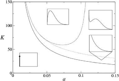
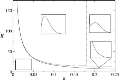
is exactly as predicted in the mean field theory, cf. Eqs. (3)-(4). However, here there are distributions of infected mouse populations underlying this mean, and our interest lies in the different shapes of these distributions in different parameter regimes, and in the additional information beyond the mean contained in these distributions. The distributions, described in detail below, are sketched in Fig. 1, where we present the phase diagrams of the system in $(K,a)$ space for fixed $b$ and $c$. The values of $b$ and $c$ have been chosen to match those used in earlier Monte Carlo simulations aguirre and/or to make most evident the different behaviors that are observed in the system.

(a) $~{}b=0.8$, $c=0.5$

(b) $~{}b=0.5$, $c=0.2$

Figure 1: Phase diagrams for the infected mouse population in $(K,a)$ space, described in detail in the text.

Various phase boundary lines are shown in Fig. 1. The solid curves in both panels are the curves $K=K_{c}$. When $K<K_{c}$ the probability distribution (30) can not be normalized because it has a nonintegrable singularity at $n_{I}=0$. Since this is a fixed point of the dynamics, the probability distribution must be interpreted as a $\delta$ function centered at zero gardiner . The insets at the lower left of each panel are a schematic of this behavior. When $K$ crosses the $K_{c}$ curve there is still a divergence at $n_{I}=0$, but the probability distribution becomes integrable and hence normalizable. The most probable value for the infected population is still zero, but nonzero values now have a finite probability and the mean value of infected mice is positive. The lower right hand insets in both panels are sketches of this behavior, which persists as a function of increasing $K$ until the carrying capacity reaches a second critical value,

$$K_{c}^{*}=\frac{2b}{b[2a-(b-c)]+\sqrt{b(b-c)[b^{2}-c(4a+b)]}}.$$ (32)

When $K$ crosses the curve $K=K_{c}^{*}$ the divergence in the distribution (30) disappears and the most probable number of infected mice moves to finite values. The curve has a divergent asymptote at $a=0$, but its behavior as a function of $a$ otherwise depends on the other parameters. If $b<2c$ then $K_{c}^{*}$ also diverges at $a=a_{c}\equiv(b-c)^{2}/b$. This is the situation in panel (a) of Fig. 1. On the other hand, if $b>2c$ then $K_{c}^{*}$ is complex when $a>a_{c}\equiv b(b-c)/4c$, thus producing the abrupt vertical boundary seen in panel (b). This second case corresponds to the parameters $b$ and $c$ in the Monte Carlo simulations of Aguirre et al. aguirre . In either case, within the region enclosed by the $K_{c}^{*}$ curve (dashed curve in the figure) the probability distribution goes to zero at the origin and has a maximum at a finite value of $n_{I}$, as shown in the upper left sketches in both panels. Both the average number of infected mice and the most probable number of infected mice are now positive. Note that we have labeled the rightmost value of $a$ on the dashed curve as $a_{c}$, whether it is an asymptote as in panel (a) or the abrupt ending point of the curve as in panel (b).

There is an additional transition curve, more subtle than the other two, drawn as the dotted curves in both panels in Fig. 1. We denote this transition curve as $K_{c}^{**}$. On the upper right hand in both panels is the sketch of the probability distribution in this region. Here the probability distribution diverges at zero, but another maximum develops at a finite number of infected mice. This maximum is found as the finite positive root of the derivative condition $dP(n_{I})/dn_{I}=0$. The dotted curves in the phase diagrams indicate the location of this transition.

(a) $a=10^{-2}<a_{c}$

(b) $a>a_{c}$

Figure 2: Ratio of the dispersion to the mean number of infected mice for $b=0.5$ and $c=0.2$.

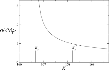
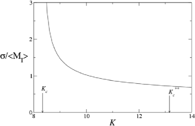
A number of points about these results deserve special highlighting. The particular behavior just described for large $K$ and $a$ (divergence at the origin and also another maximum) is entirely due to the fact that the internal fluctuations are colored. The correlation time of these fluctuations is $(b-c)^{-1}$, and the color has arisen naturally and not as an additional assumption. It is interesting to note that the Monte Carlo simulation results of Aguirre et al. aguirre exhibit a number of features that might be related to the results that we have derived here. One is that in their simulations the number of infected mice as a function of $K$ jumps discontinuously from zero to a finite number (whereas the mean field value does not). They note that an explanation for this result lies in the fact that the number of mice is discrete and that one whole mouse is needed to obtain a result different from zero (although their jump is much greater than unity). In our continuous language, the behavior they observe might reflect the abrupt transition between the $\delta$-function distribution (or the one with a maximum at the origin) to the one with a zero probability density of no infected mice as $K$ increases. Their simulations use the value $a=10^{-2}$. To support this argument further, we have plotted in Fig. 2 the ratio of the dispersion to the mean for these parameter values. The dispersion is of the order of the mean and, near the transition value $K_{c}$, the ratio actually diverges. We have elsewhere pursued the argument that a possible criterion for the likely extinction of a species is precisely that the dispersion be of the same size as the mean escudero . The substantial width of the distribution might make itself apparent in a simulation through the high likelihood of absence of the infected species. For comparison, we have also plotted the ratio of the dispersion to the mean for a value of $a>a_{c}$. The fluctuations are now decidedly smaller, even though we are in a regime of far fewer infected mice on average (as indicated by the values of $K$). It would be interesting to see whether the size of the jump in the infected mouse population at the transition would decrease in a Monte Carlo simulation with $a>a_{c}$.

Finally, we comment on three last points. One concerns the validity of the system size expansion. The total mean number of mice in the population is $K(b-c)$, and the system size expansion is valid if this number is in some sense sufficiently large (the expansion is valid if the neglected terms are small). While we have not explicitly checked the validity, in most of the regimes under discussion the number of infected mice is an order of magnitude greater than unity. Our second point is to stress that the fluctuations that lead to the distributions of infected mice are entirely due to the discrete and finite character of the total number of mice. And yet, while the ratio of the width of the distribution of total mice to the mean number of total mice, $\sigma_{M}/M$, is small in most of the phase diagram ($\sigma_{M}/M=\sqrt{(b/K)}/(b-c)$), the width of the distribution induced in the number of infected mice is relatively large (of $O(\geq 1)$) in most of the diagram. The third point is a reminder that this theory has not included the fluctuations caused directly by the fact that the number of infected mice is discrete and finite. These fluctuations would further broaden the distributions.

V Conclusions

We have considered the effect of the internal fluctuations in the total mouse population on the number of infected mice. Although these fluctuations cause no dramatic effects in the total mouse population, yielding a Gaussian distribution of relatively small variance for a sufficiently large population, these fluctuations have a rather strong effect on the distribution of infected mice. Because the fluctuations are not “direct” but instead appear indirectly through the coupling between infected and uninfected mice, the fluctuations necessarily and naturally appear as colored in the equations that describe the evolution of infected mice. This leads to a variety of effects beyond those that would be caused by simple white noise horsthemke ; katja . The mean infected population in this model is exactly that predicted in mean field. However, while the mean field model predicts one critical value of the carrying capacity parameter ($K_{c}$) such that below this value there is no infection and above this value there is, the stochastic model leads to three critical values ($K_{c}$, $K_{c}^{*}$ and $K_{c}^{**}$). The first, which occurs at the same critical value as that of the deterministic model, here corresponds to a transition between a state with no infected mice to an intermediate state in which the most probable state is still one with no infected mice but with a finite probability of infection. The second describes a transition between this intermediate state and the outbreak state, where the probability distribution that there is no infection goes to zero. The intermediate state ($K_{c}<K<K_{c}^{*}$) displays different behaviors depending on the parameter values. In particular, in some parameter ranges the intermediate state has very few infected mice. We argued that the inclusion of the internal fluctuations in the infected mouse population (which was not considered due to analytic difficulties) would probably lead to extinction of this small number of infected mice. This then means that the effective transition between non-epidemic and epidemic states may occur at $K_{c}^{*}$ rather than at $K_{c}$. We also identified another transition curve, $K_{c}^{**}$, beyond which the probability diverges at zero but where another maximum develops at a finite number of infected mice.

These features may be useful in the design of more effective prevention policies. For instance, an increase in the effective annihilation rate of the mice (by either increasing the death rate or decreasing the birth rate or both) might help because it increases the relative size of the region in parameter space in which the infected mouse population distribution has a divergence at the origin (the state of no infected mice). The most effective strategy for the control of Hantavirus outbreaks is the reduction of the carrying capacity $K$ so as to cross from one regime to another with a higher probability of no infected mice.