Three-body Interactions Improve the Prediction of Rate and Mechanism in Protein Folding Models

Abstract

Here we study the effects of many-body interactions on rate and mechanism in protein folding, using the results of molecular dynamics simulations on numerous coarse-grained $C_{\alpha}$-model single-domain proteins. After adding three-body interactions explicitly as a perturbation to a Gō-like Hamiltonian with native pair-wise interactions only, we have found 1) a significantly increased correlation with experimental $\phi$-values and folding rates, 2) a stronger correlation of folding rate with contact order, matching the experimental range in rates when the fraction of three-body energy in the native state is $\approx 20\%$, and 3) a considerably larger amount of 3-body energy present in Chymotripsin inhibitor than other proteins studied.

Understanding the nature of the interactions that stabilize protein structures and govern protein folding mechanisms is a fundamental problem of molecular biology WolynesPG95:sci ; Dobson98 ; FershtAR99:book ; MirnyL01 ; DillKA97 ; Daggett03:nat , with applications to structure and function prediction MarcotteEM99 ; HaoM99:cosb ; BonneauR01 as well as rational enzyme design BolonDN02 . Regarding folding mechanisms, protein folding has long been known to be a cooperative process, at least for smaller single-domain proteins JacksonSE98 . Experimental scenarios that lack a first-order-like folding barrier are rare GruebeleM99 , often in contrast to simulation results. There are other discrepancies between simulation and experiment. For example, while the experimental folding rates for a typical set of 18 2-state, single domain proteins (given in Methods) span $\sim 6$ orders of magnitude, simulations of coarse-grained models of the same proteins have rates that vary by about a factor of $100$, a discrepancy of 4 orders of magnitude.

How does one then quantify the sources of the barrier that controls the folding rate? The folding barrier is the residual of an incomplete cancellation of large and opposing energetic and entropic contributions, with the relative smallness of the barrier allowing folding to occur on biological time-scales Hao94 ; PlotkinSS02:quartrev12 . Among the important energetic contributions that drive folding are solvent-mediated hydrophobic forces DillKA90r , which are known to be weaker on short length scales, or low concentrations of apolar side-chains LumK99 - a scenario likely to be present when the protein is unfolded. Hence the solvent-averaged potential governing folding almost certainly contains a non-additive, many-body component. The folding free energy barrier increases as the non-additivity of interactions is increased PlotkinSS97 ; Doyle97 ; ChanHS00:pro , due to the decreased energetic correlation between the native conformation and conformations that may be geometrically similar to it.

Experimental $\phi$-values give a measure of the strength of native interactions involving a particular amino acid (residue) in the transition state FershtAR92 , thus quantifying a residue’s importance in folding. However the $\phi$-values obtained from simulations of coarse-grained protein models generally do not correlate well with the experimentally determined values. Model proteins are coarse-grained on the belief that a reduced number of degrees of freedom can capture the essentials of the folding process OnuchicJN95:pnas ; SheaJE01 ; MirnyL01 , however the less than ideal agreement with experimentally observed rates and mechanisms leads one to consider alternate forms for the coarse-grained Hamiltonian or energy function, as well as to consider more detailed all-atom models DaggetV94 ; YoungWS96 ; SnowCD02 which may contain explicit solvent as well BoczkoEM95 ; DuanY98 ; KazmirskiSL01 ; Daggett03:nat ; SnowCD02 ; GarciaAE03:pnas .

But it is also clear that coarse-grained simulations allow a study of microscopic dynamics that would not be possible by all-atom models with present-day computing power. Because we cannot yet fully analyze the statistics of folding trajectories in all-atom models, coarse-grained simulational models such as off-lattice $C_{\alpha}$ models GuoZ95 ; ZhouY99 ; ClementiC00:jmb ; VendruscoloM01 ; MirnyL01 ; KogaN01 ; SheaJE01 have been essential in elucidating protein-folding mechanisms.

We could then take the following approach: postulate a given feature thought to be present in the system and ask to what extent this feature, such as many-body potentials, must be present in the Hamiltonian of a coarse-grained model for best agreement with existing experimental data on protein folding rates and mechanisms.

I Materials and Methods

I.1 Simulation Model

Eighteen two-state folding proteins with known native structures (PDB codes 1AEY, 1APS, 1FKB, 1HRC, 1MJC, 1NYF, 1SRL, 1UBQ, 1YCC, 2AIT, 2CI2, 1PTL, 2U1A, 1AB7, 1CSP, 1LMB, 1NMG, 1SHG ) were selected for coarse-grained simulations. For all proteins except the last 5 above, rate data was available at various denaturant concentrations. These were then used for further analysis at the stability of the transition midpoint.

The simulated proteins consist of a chain of connected beads, with each bead representing the position of the $C_{\alpha}$ atom in the corresponding amino acid. The off-lattice $C_{\alpha}$ Gō model has been described in detail previously GuoZ95 ; ClementiC00:pnas ; SheaJE01 ; KogaN01 . The Hamiltonian has local and non-local parts: Bond, angle and dihedral angle potentials constitute local interactions. In the putative Gō model, pair contacts between residues in spatial proximity in the native structure constitute non-local interactions. Non-native interactions are treated by a sterically repulsive pair-potential only. Heavy atoms within a cut-off distance of $r_{c}=4.8$ Å in the native structure obtained from the PDB file are associated with a Lennard-Jones-like 10-12 potential of depth $\epsilon_{2}=-k_{\mbox{\tiny B}}T$ and a position of the minimum equal to the distance of the $C_{\alpha}$ atoms in the native structure. Let there be $N_{2}$ pair-contacts of energy $\epsilon_{2}$ in the native PDB structure. Then in an arbitrary conformation there are $QN_{2}$ contacts with energy $E_{2}\approx\epsilon_{2}\,Q\,N_{2}$, with $Q$ the fraction of native pair contacts (we account for the continuum nature of the Lennard-Jones potentials).

We let triples with heavy atoms within a cutoff distance of $4.8$ Å  in the native structure have an energy $\epsilon_{3}$. For a given protein there will then be $N_{3}$ 3-body contacts present in the PDB native structure, with total $3$-body energy $\epsilon_{3}N_{3}$. An arbitrary structure then has a 3-body contribution to the energy of $E_{3}\equiv\epsilon_{3}\,Q_{3}\,N_{3}$, where $Q_{3}$ is the fraction of native triples present in that conformation. Three-body interactions are again Gō-like; the remaining bond, angle, dihedral, and non-native interaction energies are all unchanged.

When both pair-wise and 3-body interactions are present, the native non-local part of the energy becomes:

$$E_{\mbox{\tiny{NL}}}(\alpha)=(1-\alpha)E_{2}+\alpha E_{3}.$$ (1)

The free parameter $\alpha$ ($0\leq\alpha\leq 1$) controls the relative contribution of two- and three-body interactions. The energy per triple is assigned as $\epsilon_{3}=\epsilon_{2}\,N_{2}/N_{3}$, to preserve overall native stability.

Dense sampling is obtained from long simulations with a purely 2-body Gō Hamiltonian at the transition mid-point (e.g. for CI2 the simulation time corresponds to about $3$ seconds, as determined from the number of folding and unfolding events). From histograms of the number of states at a given fraction of native contacts $Q$, the free energy $F(Q)$ can be constructed. All simulated free energy profiles displayed a single dominant barrier. All proteins are considered at their transition mid-points only, where the unfolded and folded free energies are equal: $F_{\mbox{\tiny U}}=F_{\mbox{\tiny F}}$ (figure 1 A).

Three-body energies are treated as a perturbation on the Hamiltonian. The new free energy is given by the exact expression:

$$\frac{F(Q,\alpha)}{k_{\rm B}T}=-\ln\frac{\sum_{i}\mbox{e}^{-\Delta E_{i}(\alpha)/k_{\rm B}T}\,\Delta(Q^{(i)},Q)}{\sum_{i}e^{-\Delta E_{i}(\alpha)/k_{\rm B}T}},$$ (2)

where the sum is on all sampled conformations $i$, $\Delta(Q^{(i)},Q)$ is a delta function that selects only those states where $Q^{(i)}=Q$, and $\Delta E(\alpha)=E_{\mbox{\tiny{NL}}}(\alpha)-E_{2}$.

I.2 Calculated $\phi$-values

Simulated kinetic $\phi$-values are given by Onuchic96 :

$$\phi_{i}=\frac{\langle n_{i}\rangle_{\neq}-\langle n_{i}\rangle_{U}}{\langle n_{i}\rangle_{F}-\langle n_{i}\rangle_{U}},$$ (3)

where $\langle n_{i}\rangle$ is the thermal mean value of number of contacts for residue $i$, and the $\neq$, $U$ and $F$ subscripts refer to the transition state, unfolded state and folded state ensembles respectively.

We first compare simulated and experimental $\phi$-values using the thermal transition state ensemble (TTSE) around the free energy barrier peak, i.e. $\left|F-F^{\neq}\right|/\Delta F^{\neq}\leq 0.2$ was used to define a width $\Delta Q$ of the barrier peak (shaded in figure 1 A). Conformations within this range were taken to be the TTSE, and were used to calculate $\phi$ values from equation 3. The validity of the TTSE was checked for CI2 and SH3 with a comparison of $\phi$-values using the kinetic transition state ensemble (KTSE), selected as having a folding probability $p_{\mbox{\tiny FOLD}}$ of roughly $1/2$ DuR98:jcp . Conformations in the TTSE were used as initial conditions for 100 simulations which were terminated when the protein folded or unfolded. Those conformations that had a $p_{\mbox{\tiny FOLD}}$ within $0.5\pm 1/\sqrt{100}$ were taken as the KTSE. For CI2 (SH3) we found $315$ ($283$) KTSE configurations from a total of $2359$ ($2078$) TTSE configurations.

Other reaction coordinates were helpful in determining the kinetic transition state ensemble by constructing multi-dimensional reaction surfaces. To this end we found a contact-order weighted variant of $Q$ to be useful, which for any configuration $\nu$ is given by:

$$Q_{\mbox{\tiny{CO}}}^{\nu}=\frac{\sum_{i<j}\left|i-j\right|\Delta_{ij}^{\nu}\Delta_{ij}^{N}}{\sum_{i<j}\left|i-j\right|\Delta_{ij}^{N}}$$ (4)

where the sum is over all $C_{\alpha}$ atoms, and $\Delta_{ij}^{\nu}$ and $\Delta_{ij}^{N}$ are unity if residues $i$ and $j$ are in contact in conformations $\nu$ and the native structure respectively, otherwise they are zero.

We determined $\phi$-values in the presence of three-body interactions analogously to eq. (3). Under some simplifying assumptions (e.g. requiring that the $\phi$-value that is independent of the perturbation energies):

$$\phi_{i}^{(\alpha)}=\frac{(1-\alpha)\,(\langle n_{i}\rangle_{\neq}^{(\alpha)}-\langle n_{i}\rangle_{U}^{(\alpha)})\,N_{3}+\alpha\,(\langle m_{i}\rangle_{\neq}^{(\alpha)}-\langle m_{i}\rangle_{U}^{(\alpha)})\,N_{2}}{(1-\alpha)\,(\langle n_{i}\rangle_{F}^{(\alpha)}-\langle n_{i}\rangle_{U}^{(\alpha)})\,N_{3}+\alpha\,(\langle m_{i}\rangle_{F}^{(\alpha)}-\langle m_{i}\rangle_{U}^{(\alpha)})\,N_{2}}.$$ (5)

Here $m_{i}$ is the number of three body interactions in which monomer $i$ is involved, and superscript $(\alpha)$ indicates averaging the ensembles ($\neq$, $U$, $F$) in the presence of 3-body energy. When $\alpha\rightarrow 0$, (5) reduces to (3).

I.3 Miyazawa-Jernigan-based Models

The effect of heterogenity in the model was also studied by interpolating between the Gō model and the Miyazawa-Jernigan (MJ) models by varying the free parameter $\alpha$ between zero (Homogeneous Gō model) and unity (MJ model). The contact energy for any pair of residues (not necessarily native) is then:

$$\epsilon_{ij}=(1-\alpha)\epsilon_{2}+\alpha\epsilon_{ij}^{\rm MJ}\>,$$ (6)

where $\epsilon_{2}$ is as above, and $\epsilon_{ij}^{\rm MJ}$ was proportional to the MJ interaction energy MiyazawaS96 between the residue types of $i$ and $j$, scaled by a factor to ensure the energy of the native structure is $\alpha$-independent. An interpolation between a uniform Gō model and a heterogeneous Gō model with native contact energies given by MJ parameters was also considered.

I.4 Contact Order and Statistical Significance

Absolute contact order is the average sequence separation between residues having native contacts Plaxco98 : $aCO=M^{-1}\sum_{i>j}|i-j|$, where $M$ is the total number of native contacts. Relative contact order is scaled again by chain length $N$: $rCO=aCO/N$.

Statistical significance or $P$-value is the probability to achieve a given correlation coefficient, $r$, assuming random data: $P=\mbox{erf}(|r|\sqrt{N/2})$. Small data sets almost always have fairly large $P$, even if $r$ is large. Large data sets may still have small $P$ even if the correlation is weak, which would still indicate a systematic effect.

II RESULTS

II.1 Protein folding rates

Here we considered the effect of introducing a three-body potential to an off-lattice two-body Gō model studied previously ClementiC00:pnas ; SheaJE99 ; KogaN01 . Eighteen mentioned single-domain proteins that are known to fold by a two-state mechanism were selected, and coarse-grained so that each amino acid corresponds to a bead at the position of the $C_{\alpha}$ atom. Long simulations at the folding temperature $T_{f}$ for a subset of the proteins showed a single exponential distribution of first passage times: $P(\tau)\sim\exp(-\kappa t)$. For these proteins the simulated log folding rate, $\mbox{log}(\kappa)$, correlated very strongly (r=0.997) with the free energy barrier height $\Delta F^{\neq}$ , indicating that $\Delta F^{\neq}$ was an accurate predictor of the rate for the simulated Gō models. We subsequently assume this proportionality between $\Delta F^{\neq}$ and $-\mbox{log}(\kappa)$ for all simulated proteins, referring to $\exp(-\Delta F^{\neq}/k_{\mbox{\tiny B}}T)$ as the “effective rate”.

The above mentioned discrepancy between the effective protein rates for our data set and the experimentally determined rates for the same proteins motivates an investigation of the effect of many-body interactions on rates. When a portion of the total energy is attributable to many-body interactions, energetic gain is not achieved until a larger amount of native structure is present, with a correspondingly larger entropic cost. Several polymer loops must be simultaneously closed during folding to receive energetic gain. This effect enhances the dependence of rate on contact order, increasing the range over which rates vary.

By attributing a fraction $\alpha$ of the native energy to triples in the native structure, we studied the effects of three-body interactions by varying this single parameter (see Methods). The effects on the free energetic potential surface for several proteins are shown in figure 1.

As the fraction of 3-body energy is increased, the correlation of the simulated effective rates with both absolute and relative contact order increases (figure 2 a,b). This effect has also been seen in lattice protein models KayaH03:prots2 ; JewettAI03 . We can also quantify how much 3-body energy, at the residue level, reproduces the experimental dispersion in rates for single-domain proteins. The simulated effective rates span 6 orders of magnitude when approximately $20\%$ of the energy in the native state of the coarse-grained protein is due to 3-body interactions.

Rates simulated with a 2-body Hamiltonian do not correlate significantly with experimentally determined rates at $25^{o}C$ (figure 2 C). We can remove the effects due to variations in stability and reflect the conditions in the simulations by taking instead the rate data at the various transition midpoints (after the addition of GdHCl). We then found the correlation significantly increased to $r=0.64$, $p=0.018$. Adding 3 body energy in the simulations increases the correlation with the experimental rates (at the transition midpoints) still further, with the best correlation achieved when $\alpha=10\%$ (see figure 2d).

These results strongly suggest that 1) stability is an important determinant of folding rate, 2) many-body energy is present in the energy functions of real proteins, and 3) Gō or Gō-like models (which ignore non-native interactions) can predict experimental rates, illustrating the minor importance of non-native interactions in governing folding barriers.

The correlation of log rates with $rCO$ also improves as $\alpha$ is increased from zero, however the correlations are modest, increasing from ($r=0.29$, $P=0.24$) at $\alpha=0$ to a best correlation of ($r=-0.44$, $P=0.08$) at $\alpha=10\%$ (data not shown).

II.2 Testing pair interaction matrices

The correlation between experimental and simulational $\phi$-values for a 2-body Hamiltonian ($r_{0}$, $P_{0}$) was typically not statistically significant (see table I), with the exception of SH3. Rank ordered measures of correlation such as Kendall’s tau, which are insensitive to the precise values of the data, generally do not improve the agreement (table II). We also checked whether simulations with a 2-body Hamiltonian could accurately predict residues that had higher-$\phi$ values. This was done by weighting the statistical averaging in the correlation coefficient by the experimental $\phi$-value itself as a Jacobian factor. Implementing this recipe did not substantially increase the correlation coefficient, and in fact decreased it in the cases of AcP and CI2 (table I). Similar results were obtained by implementing a simple cut-off imposing a lower bound for relevant experimental $\phi$-values (data not shown).

The experimental data can be used to test energy functions characterizing pair-interactions at the amino acid level, such as the Miyazawa-Jernigan (MJ) matrix MiyazawaS96 . We investigated whether MJ interaction parameters improved the simulational predictions of $\phi$-values, by interpolating between a homogeneous Gō model and a model with pair interactions (between all residues) governed by MJ parameters (see equation (6)). We also interpolated between a homogeneous Gō model and a heterogeneous Gō model with native interaction parameters determined from the MJ matrix.

Results are shown for two proteins in figure 3. For CI2 and SH3, no improvement in the correlation with experimental data was seen by implementing this procedure. Table I shows the results for the comparison between experimental $\phi$-value data and $\phi$-values obtained from a pairwise MJ Hamiltonian. In general if correlations increased by interpolating toward MJ parameters they did so only modestly- only in the case of protein L did the improvement reach statistical significance ($P=1\%$, see table I).

To check of the validity of the recipe of interpolating toward MJ parameters, we compared the largest improvement in correlation $(r_{\alpha^{*}}-r_{o})$ with the value $\alpha^{*}$ of three body energy required to achieve that correlation. This tests whether the poorness of the original correlation was due to the absence of MJ coupling energies. We found that $(r_{\alpha^{*}}-r_{o})$ itself correlated well with $\alpha^{*}$, however the statistical significance was not particularly strong, and the slope measuring the degree of improvement was not particularly high (see figure 4).

II.3 Testing three-body interactions

The experimental data can also be used as a benchmark to test what amount of 3-body energy in the Hamiltonian of the coarse-grained model gives best agreement with experimental $\phi$-values . We examined this question for the 5 proteins in table I, by measuring the correlation between the experimentally obtained $\phi$-values, and $\phi$-values of the same residues determined from simulations, with conditions ranging from between a pair-wise interacting Gō model protein, and one governed exclusively by 3-body interactions at the residue level (see methods).

As the strength of 3-body interactions increased from zero, the correlation coefficient also increased, for all proteins studied (see fig. 3 and table I). An exceptional case was SH3, which showed only a modest increase in correlation for the kinetically determined transition state ensemble, and no increase for the thermal transition state ensemble. The fraction $\alpha^{\ast}$ of native 3-body energy that gave best agreement with experimental data varied from protein to protein, but correlated strongly with the increase in agreement with experimental data (see table I). That is, the improvement in correlation $(r_{\alpha^{*}}-r_{o})$ itself correlated very strongly with $\alpha^{\ast}$ ($r=0.97$, $P=0.005$), further supporting the notion that the poorness of the original agreement was due at least in part to the absence of many-body forces.

For a protein such as CI2 with large fraction of 3-body energy, the transition states in the presence of 3-body interactions is significantly different than the 2-body transition state. For CI2, the root mean square distance (RMSD) between all $315$ structures in the kinetic transition state ensemble (KTSE) was found for both the 2-body and 2+3-body (at $\alpha^{*}$) cases. Shown in figure 5A, B is the “most representative” transition state structure for the 2-body and 2+3-body cases respectively, defined as having the minimal Boltzmann-weighted RMSD (minimum over structure $i$ of $\sum_{j}\,p_{j}(\mbox{RMSD})_{ij}$) to all others in the KTSE. The 2-body case shows more overall secondary structure, in particular more $\alpha$-helix, but less $\beta$-sheet. The $Q$, $Q_{\mbox{\tiny{CO}}}$ (see methods), and $R$ (RMSD from the native structure) values for the structures in figure 5A,B are $Q^{\mbox{\tiny{(A)}}}=0.54$, $Q^{\mbox{\tiny{(B)}}}=0.49$, $Q_{\mbox{\tiny{CO}}}^{\mbox{\tiny{(A)}}}=0.41$, $Q_{\mbox{\tiny{CO}}}^{\mbox{\tiny{(B)}}}=0.29$, and $R^{\mbox{\tiny{(A)}}}=5.5$ Å, $R^{\mbox{\tiny{(B)}}}=11$ Å. This indicates that the 2+3-body transition state is less structured than the pure 2-body transition state. However, kinetically they are about the same distance from the native structure, with $p_{\mbox{\tiny FOLD}}$ values $p_{\mbox{\tiny FOLD}}^{\mbox{\tiny{(A)}}}=0.55$, $p_{\mbox{\tiny FOLD}}^{\mbox{\tiny{(B)}}}=0.53$ note:pfold . They have a RMSD of $7.8$ Å between them, so they are structurally distinct from each other. The average RMSD values from the native for the top 4 transition state structures for the 2-body and (2+3)-body cases are $\overline{R}^{\mbox{\tiny{(2)}}}=6.3$ Å, and $\overline{R}^{\mbox{\tiny{(2+3)}}}=8.5$ Å, again confirming less native structure in the more accurate transition state containing 3-body interactions. Interestingly, the high-$\phi$ residue 34 has more local secondary structure in the pure 2-body case than at $\alpha^{*}$. It also has no triples in the native state. Its high $\phi$-value in the presence of 3-body interactions is the result of correlations with other triples made in the transition state.

The procedure of adding 3-body interactions was repeated considering only residues in the hydrophobic core of native structure, in this case buried with less than $\approx 30\%$ accessible surface area using the Swiss PDB algorithm. (http://www.expasy.org/spdbv). We saw qualitatively the same effect, but the change in correlation coefficient was less pronounced, increasing to about $0.42$ for CI2 for example. This implies that coarse-grained model proteins with effective solvent-averaged interactions have many-body interactions involving residues on the surface as well.

III Discussion

The above results suggest that many-body interactions can play a significant role in governing the folding mechanisms of 2-state proteins when described at the residue level. This seems quite evident upon comparing the statistical significance columns in table I or table II for the pure 2-Body Hamiltonian and the 2+3-body Hamiltonian at $\alpha^{*}$. In essentially all cases, many-body interactions helped to establish consistency with protein folding experiments. Some proteins showed dramatic improvement, others mild improvement, so proteins may be additionally classified through this effect. The value of $\alpha^{\ast}$ may be used as an indication of the importance of many-body interactions in governing the folding mechanism for a given protein, as for example the proteins are ranked in tables I and II.

Experimental rates vary by about 4 orders of magnitude more than rates obtained from coarse-grained models using 2-body Hamiltonians. However a modest 3-body component to native stability (about 20% on average) was sufficient to reproduce the experimental variability in folding rates. It is an open question as to how large the many-body component might be in finer-scale and all-atom models of proteins. Ab initio studies of interaction energies and reconfiguration barriers in water clusters suggest they can be quite significant MiletA99 .

For FKBP, protein L, and CI2 the correlation between experimental and simulational $\phi$ values goes from insignificant to significant as 3-body interactions are added. In the case of CI2, the agreement between simulations with a 2-body energy function and experimental data was the poorest of the proteins studied, the fraction of 3-body energy at best agreement was the largest, and the improvement in correlation coefficient the most dramatic. In the case of SH3 on the other hand, the folding mechanism appears to be governed more by topology than by energetic considerations. In some sense this is an exception that proves the rule, since previous evidence supported a folding mechanism dominated by topological considerations RiddleDS99 ; MartinezJC99 .

Interestingly, muscle acylphosphatase had the poorest improvement in mechanism prediction by adding 3-body interactions, as measured by the correlation coefficient. Its original $\phi$-correlation for a 2-body Gō model was the second poorest after CI2. It also required the largest amount of Miyazawa-Jernigan interactions for best agreement with experimental $\phi$-values , but still correlated poorly even at best agreement. Intriguingly it is also the slowest known 2-state folder at present, yet a good 2-state folder with no intermediates ChitiF99 . The slow folding is likely due to large contact order however, and it would be interesting in the future to apply the 3-body recipe to a topologically similar but faster folding protein such as human procarboxypeptidase A2. On the other hand, the improvement for AcP as measured by Kendall’s tau does in fact become statistically significant, and suggests a large 3-body component. We are inclined to take this more robust measure of statistical significance more seriously. The discrepancy of $r$ and $\tau$ indicates some large outliers in $\phi$-values , likely due to variations in native stabilizing interactions, which may exist for functional reasons. These fluctuations in native interaction strength are not captured by the uniform Gō model and 2+3-body models.

The largest improvement in correlation $(r_{\alpha^{*}}-r_{o})$ with the value of interpolation parameter $\alpha^{*}$ required to achieve that correlation was used as a measure to test the validity of the 3-body and Miyazawa-Jernigan interpolation recipes. The results for the 3-body interpolation recipe showed a strong statistically significant correlation with large slope indicating large rate of improvement. The results for the heterogeneous MJ Gō model also showed improvement, however with smaller slope and smaller statistical significance. It is noteworthy that for the case where CI2, where the 3-body recipe does the best, the MJ recipe failed to improve the agreement with experiment.

For CI2, the transition state in the presence of 3-body interactions shows less overall native structure than the purely 2-body transition state, in spite of the better agreement with experimental $\phi$-values for the 3-body case. However it is not clear that this will be a general rule. In both cases the transition state consists largely of a disordered form of the native topology, sufficiently disordered to be kinetically balanced between the folded and unfolded states.

The low levels of agreement between experiment and simulation for 2-body Hamiltonians told a somewhat cautionary tale. While a large body of evidence leaves little doubt as to the importance of native topology in governing folding mechanism, these results should serve to show that realistic aspects of the energy function, such a many-body component to native stability, should not be ignored.

IV Acknowledgments

S. S. P. acknowledges support from the Natural Sciences and Engineering Research Council and the Canada Research Chairs program. We thank Cecilia Clementi and Baris Oztop for helpful discussions.

Table 1: Two-body and Three-body characterization of proteins studied

	Gō MODEL		MJ MODEL			MJ-Gō MODEL			3-BODY MODEL
Proteins (PDB)	$r_{0}$	$P_{0}$	$\alpha^{*}$	$r_{\alpha^{*}}$	$P_{\alpha^{*}}$	$\alpha^{*}$	$r_{\alpha^{*}}$	$P_{\alpha^{*}}$	$\alpha^{*}$	$r_{\alpha^{*}}$	$P_{\alpha^{*}}$
SH3 (1SRL)	0.58	0.0003	0%	0.59	0.0003	5%	0.59	0.0002	5%	0.60	0.0001
FKBP (1FKB)	0.32	0.17	10%	0.41	0.07	20%	0.38	0.1	10%	0.43	0.057
AcP (1APS)	0.12	0.58	50%	0.35	0.1	30%	0.30	0.16	15%	0.32	0.14
Protein L (2PTL)	0.18	0.25	20%	0.38	0.01	30%	0.38	0.01	15%	0.53	0.00027
CI2 (2CI2)	-0.10	0.56	0%	-0.017	0.92	0%	-0.017	0.92	35%	0.57	0.0004

					3-BODY MODEL				HIGH-$\phi$ WEIGHTING
Continue	$N$	$N_{2}$	$N_{3}$	$n$	$\alpha^{*}$	$\Delta F^{\neq}_{\alpha^{*}}$	$\frac{\Delta F^{\neq}_{\alpha^{*}}}{\Delta F^{\neq}_{0}}$	$\frac{E_{\rm 3B}^{\rm\neq}}{E_{\rm tot}^{\rm\neq}}$	$\widetilde{r}_{0}$	$\widetilde{P}_{0}$
SH3 (1SRL)	56	128	32	35	5%	3.8 $\pm$ 0.2	1.4	2.6%	0.65	$2.7\times 10^{-5}$
FKBP (1FKB)	107	299	111	20	10%	10 $\pm$ 0.8	1.5	5.5%	0.37	0.10
AcP (1APS)	98	257	97	23	15%	14 $\pm$ 2.0	2.2	8.9%	-0.02	0.91
Protein L (2PTL)	62	126	30	41	15%	6.2 $\pm$ 0.5	2.8	3.3%	0.26	0.10
CI2 (2CI2))	65	148	54	35	35%	17 $\pm$ 3.5	3.4	13%	-0.43	0.01

Table 2: Kendall’s $\tau$ and Statistical significance between experiment and simulation

	Gō MODEL		3-BODY MODEL
Proteins (PDB)	$\tau_{0}$	$P_{0}$	$\alpha^{*}$	$\tau_{\alpha^{*}}$	$P_{\alpha^{*}}$
SH3 (1SRL)	0.42	0.00044	0%	0.42	0.00044
FKBP (1FKB)	0.27	0.10	10%	0.31	0.055
Protein L (2PTL)	0.14	0.19	20%	0.36	0.00069
AcP (1APS)	0.14	0.37	25%	0.33	0.027
CI2 (2CI2)	0.042	0.72	35%	0.40	0.0008

.

FIGURE CAPTIONS

Figure: 1
The folding barrier height $\Delta F^{\neq}$ increases with increasing three-body contribution to the energy $\alpha$. Inset (A) shows the free energy vs. the fraction of native contacts $Q$ for CI2, for 3 values of $\alpha$. Main panel shows the barrier vs. $\alpha$ for 4 proteins selected from table I. Inset (B): the average slope of $\Delta F^{\neq}$ vs. $\alpha$ correlates strongly with the number of $3$-body interactions in the native state ($r=0.89$, $p=10^{-6}$). Therefore the barriers in the main panel increase at different rates due to differing numbers of triples formed in the transition states of the various proteins- more native triples typically means a larger $3$-body contribution to the barrier. The shaded region in inset (A) corresponds to the thermal transition state ensemble described in the methods section. In general this ensemble depends on $\alpha$.

Figure: 2
Comparison of simulated and experimental rates. (A): Simulated folding barriers (effectively measuring log folding rates for 18 proteins listed in methods) for a pair-wise interacting Gō model correlate well with absolute contact order ($aCO$) KogaN01 . (B): Simulated folding barriers show an increased correlation with $aCO$, when the fraction of native three-body energy is such that the dispersion in effective simulated rates matches the experimental dispersion for this data set ($\alpha=20\%$). Rates now span $5.7$ decades, in contrast to $2$ decades for a pure 2-Body Hamiltonian (dashed line in (B) is the best fit line in (A)). (C): For $13$ of the $18$ proteins (see methods for a list), rate data was available for various different denaturant concentrations. These proteins were used for the analysis in figures C and D. Panel (C) shows that for these proteins, the simulated effective log rates do not correlate significantly with the experimental rate data at $25^{o}\,C$. (D): Tuning the rate data to the transition midpoints and introducing 3-body energy in the native state, we saw a significant increase in the correlation between experimental and simulated rate data, with best correlation when $\alpha=10\%$.

Figure: 3
Comparison of the agreement of $\phi$-values between simulation and experiment for (A) CI2, and (B) src SH3. Green curves in A and B show the correlation coefficient and statistical significance (insets) for $\phi$-values derived from the thermal transition state (TTSE) in the simulations, as the Hamiltonian was continuously changed from a uniform Gō model to one with pair interactions governed by Miyazawa Jernigan parameters (the curve shown in inset A is the statistical significance of the anti-correlation in the main panel) - see equation (6). No improvement was seen for CI2 or SH3 by implementing this recipe. Red and Blue curves show the correlation coefficient and statistical significance between experimental and simulated $\phi$-values as a function of the fraction $\alpha$ of three-body energy in the native state. Blue curves correspond to TTSE, Red curves- kinetic transition state ensemble (KTSE). For CI2 the improvement as $\alpha$ is increased is dramatic, with best agreement with experiment around $35\%$ 3-body energy. On the other hand, SH3 was exceptional in that it showed the opposite trend, with best agreement for a purely pair-wise interacting model for the TTSE and $\alpha=5\%$ for the KTSE. All other proteins studied were bracketed by these two extremes- they showed moderate components of 3-body energy, with moderate to large increases in correlation coefficient (table I).

Figure: 4
Plot of the largest improvement in correlation $(r_{\alpha^{*}}-r_{o})$ vs. the value of interpolation parameter $\alpha^{*}$ required to achieve that correlation. Energy functions are interpolated toward a 3-body Gō model (eq. (1)) and 2-body models with Miyazawa-Jernigan energetic parameters (eq. (6)). The slope and correlation indicate the validity of the interpolation procedure. Adding 3-body energies gives a slope of $2.2$, and $(r,P)=(0.97,0.005)$. Adding a MJ component to the pair interaction energies gives a slope of $0.29$ but a fit that is not statistically significant: $(r,P)=(0.83,0.38)$. Restricting the MJ component to native interaction energies gives a statistically significant fit, $(r,P)=(0.956,0.044)$, but with a shallow slope ($0.78$) indicating only moderate improvement.

Figure: 5
The “most representative” transition state structure for the 2-body (A) and 2+3-body (B) cases of CI2, defined as the structure having minimal Boltzmann-weighted RMSD to all other structures in the KTSE (see text). (left column: representation showing secondary structure, right columns: stereographic views superimposed on the native structure (structures generated with molmol)). The 2-body case shows more overall secondary structure, in particular more $\alpha$-helix, but less $\beta$-sheet. (C): $\phi$-value vs. residue index for CI2, for experiment (Blue), simulated pair-wise Gō model (light blue background), and 2+3-body Gō model (Red). The average $\phi$-values for the various energy functions are $\overline{\phi}^{\mbox{\tiny{(Expt)}}}=0.25$, $\overline{\phi}^{\mbox{\tiny{(2)}}}=0.40$, $\overline{\phi}^{\mbox{\tiny{(2+3)}}}=0.33$, again confirming the more accurate 2+3-body transition state is less structured. It is worth noting that native state is more stable in the experiments than in the simulations- the native stability is fixed at the transition midpoint in the simulations, regardless of the value of $\alpha$.

.

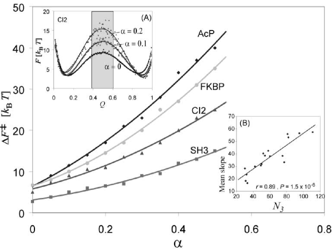
Figure 1:

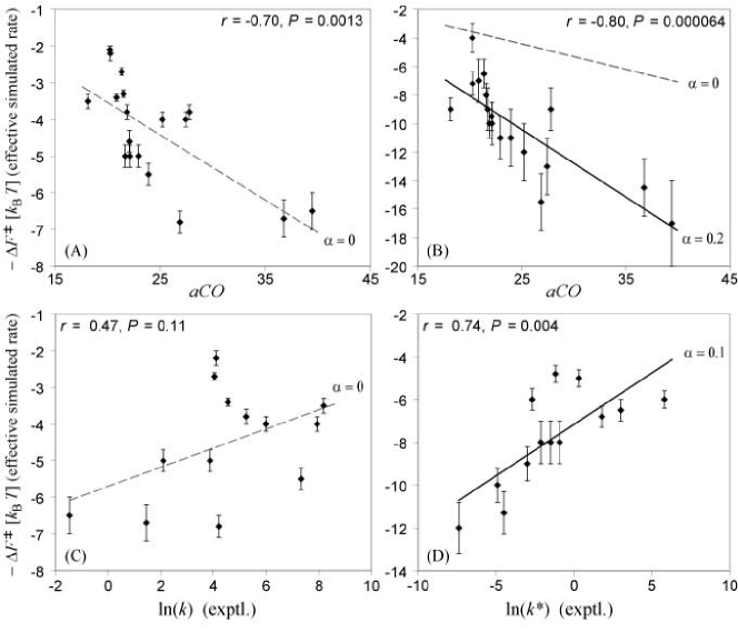
Figure 2:

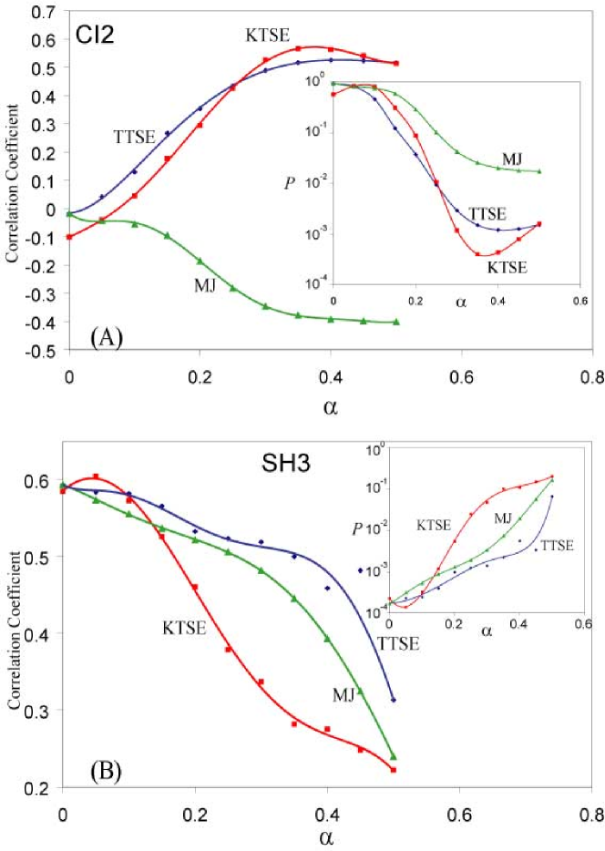
Figure 3:

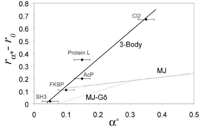
Figure 4:

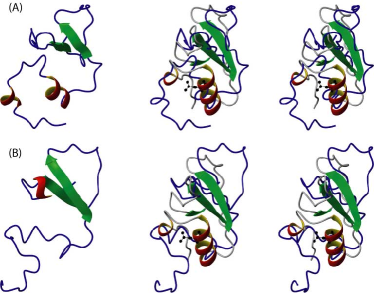
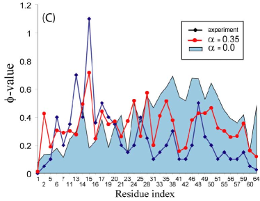
Figure 5:

References

- (1) Wolynes, P. G., Onuchic, J. N., & Thirumalai, D. (1995) Science 267, 1619–1620.
- (2) Dobson, C. M., Sali, A., & Karplus, M. (1998) Angew Chem Int Ed Engl 37, 868–893.
- (3) Fersht, A. R. (1999) Structure and mechanism in protein science (W. H. Freeman and Co., New York), First edition.
- (4) Mirny, Leonid & Shakhnovich, Eugene (2001) Annu Rev Biophys and Biomol Struct 30, 361–396.
- (5) Dill, K. A. & Chan, H. S. (1997) Nat. Struct. Biol. 4, 10–19.
- (6) Daggett, V. & Fersht, A. R. (2003) Nat Rev Mol Cell Bio 4, 497–502.
- (7) Marcotte, E. M., Pellegrini, M., Thompson, M. J., Yeates, T. O., & Eisenberg, D. (1999) Nature 402, 83–86.
- (8) Hao, Ming-Hong & Scheraga, H. (1999) Curr Opinion Struct Biol 9, 184–188.
- (9) Bonneau, R. & Baker, D. (2001) Annu. Rev. Bioph. Biom. 30, 173–189.
- (10) Bolon, D. N., Voigt, C. A., & Mayo, S. L. (2002) Curr Opinion Struct Biol 6, 125–129.
- (11) Jackson, Sophie E. (1998) Folding and Design 3, R81–R91.
- (12) Gruebele, M. (1999) Annu Rev Phys Chem 50, 485–516.
- (13) Hao, Ming-Hong & Scheraga, Harold A. 5 May (1994) J. Phys. Chem. 98(18), 4940–4948.
- (14) Plotkin, S. S. & Onuchic, J. N. (2002) Quart. Rev. Biophys. 35(2), 111–167 and 205–286.
- (15) Dill, Ken A. (1990) Biochemistry 29(31), 7133–7155.
- (16) Lum, K., Chandler, D., & Weeks, J. D. (1999) J Phys Chem 103(22), 4570–4577.
- (17) Plotkin, S. S., Wang, J., & Wolynes, P. G. (1997) J Chem Phys 106, 2932–2948.
- (18) Doyle, R., Simons, K., Qian, H., & Baker, D. (1997) Proteins: Struct. Funct. and Genetics 29, 282–291.
- (19) Chan, H. S. (2000) Proteins 40, 543–571.
- (20) Fersht, A. R., Matouschek, A., & Serrano, L. (1992) J Mol Biol 224, 771–782.
- (21) Onuchic, J. N., Wolynes, P. G., Luthey-Schulten, Z., & Socci, N. D. (1995) Proc Nat Acad Sci USA 92, 3626–3630.
- (22) Shea, J. E. & Brooks III, C. L. (2001) Annual Review of Physical Chemistry 52, 499–535.
- (23) Daggett, V. & Levitt, M. (1994) Curr Opinion Struct Biol 4, 291–295.
- (24) Young, W. S. & Brooks III, C. L. (1996) J Mol Biol 259, 560–572.
- (25) Snow, C. D., Nguyen, H., Pande, V. S., & Gruebele, M. (2002) Nature 420, 102–106.
- (26) Boczko, E. M. & Brooks III, C. L. (1995) Science 269, 393–396.
- (27) Duan, Y. & Kollman, P. A. (1998) Science 282, 740–744.
- (28) Kazmirski, S. L., Wong, K-B, Freund, S. M., Tan, Y-J, Fersht, A. R., & Daggett, V. (2001) Proc Nat Acad Sci USA 98, 4349–4354.
- (29) Garcia, Angel E. & Onuchic, Jose N. (2003) PNAS 100(24), 13898–13903.
- (30) Guo, Z. & Thirumalai, D. (1995) Biopolymers 36, 83–102.
- (31) Zhou, Y. & Karplus, M. (1999) Nature 401, 400–403.
- (32) Clementi, C., Nymeyer, H., & Onuchic, J. N. (2000) J Mol Biol 298, 937–953.
- (33) Vendruscolo, M., Paci, E., Dobson, C. M., & Karplus, M. (2001) Nature 409(2), 641–645.
- (34) Koga, N. & Takada, S. (2001) J Mol Biol 313, 171–180.
- (35) Clementi, Cecilia, Jennings, P. A., & Onuchic, J. N. (2000) Proc Nat Acad Sci USA 97, 5871–5876.
- (36) Onuchic, J. N., Socci, N. D., Luthey-Schulten, Z., & Wolynes, P. G. (1996) Folding and Design 1, 441–450.
- (37) Du, R., Pande, V. S., Grosberg, A. Yu., Tanaka, T., & Shakhnovich, E. S. (1998) J Chem Phys 108, 334–350.
- (38) Miyazawa, S. & Jernigan, R. L. (1996) J Mol Biol 256, 623–644.
- (39) Plaxco, K. W., Simons, K. T., & Baker, D. (1998) J Mol Biol 277, 985–994.
- (40) Shea, J. E., Onuchic, J. N., & Brooks III, C. L. (1999) Proc Nat Acad Sci USA 96, 12512–12517.
- (41) Kaya, H. & Chan, H. S. (2003) Proteins-structure Function Genetics 52.
- (42) Jewett, A. I., Pande, V. S., & Plaxco, K. W. (2003) J Mol Biol 326, 247–253.
- (43) Riddle, D. S., Grantcharova, V. P., Santiago, J. V., Alm, E., Ruczinski, I., & Baker, D. (1999) Nat. Struct. Biol. 11, 1016–1024.
- (44) Fulton, K. F., Main, E. R. G., Daggett, V., & Jackson, S. E. (1999) J Mol Biol 291, 445–461.
- (45) Chiti, F., Taddei, N., White, P. M., Bucciantini, M., Magherini, F., Stefani, M., & Dobson, C. M. (1999) Nature Struct Biol 6(11), 1005–1009.
- (46) Itzhaki, L. S., Otzen, D. E., & Fersht, Alan R. (1995) J Mol Biol 254, 260–288.
- (47) Kim, D. E., Fisher, C., & Baker, D. (2000) J Mol Biol 298, 971–984.
- (48) Note however that values are only calculated in the presence of the 2-body Hamiltonian, so the KTSE is only approximate in the presence of a 2+3 body Hamiltonian .
- (49) Milet, A., Moszynski, R., Womer, P. E. S., & Avoird, A. van der (1999) J. Phys. Chem. A 103(34), 6811–6819.
- (50) Martinez, J. C. & Serrano, L. (1999) Nature Struct. Biol. 6, 1010–1016.