Sampling rare switching events in biochemical networks

Abstract

Bistable biochemical switches are ubiquitous in gene regulatory networks and signal transduction pathways. Their switching dynamics, however, are difficult to study directly in experiments or conventional computer simulations, because switching events are rapid, yet infrequent. We present a simulation technique that makes it possible to predict the rate and mechanism of flipping of biochemical switches. The method uses a series of interfaces in phase space between the two stable steady states of the switch to generate transition trajectories in a ratchet-like manner. We demonstrate its use by calculating the spontaneous flipping rate of a symmetric model of a genetic switch consisting of two mutually repressing genes. The rate constant can be obtained orders of magnitude more efficiently than using brute-force simulations. For this model switch, we show that the switching mechanism, and consequently the switching rate, depends crucially on whether the binding of one regulatory protein to the DNA excludes the binding of the other one. Our technique could also be used to study rare events and non-equilibrium processes in soft condensed matter systems.

Biochemical switches are essential for the functioning of living cells. These switches are networks of chemical reactions that exhibit more than one stable steady state; in the presence of noise, flipping can occur between these states. Well-characterized examples include the lysis-lysogeny switch in bacteriophage $\lambda$ ptashne and the lac repressor in E. Coli muller ; oudenaarden ; vilar . Experimental and theoretical studies have established the presence of bistability in other biochemical networks, including those regulating the cell cycle and developmental fate pomerening ; sha ; ferrell1 ; xiong ; angeli ; ferrell2 . In addition, synthetic switches have been constructed in vivo gardner ; atkinson ; becskei1 .

Computational modeling has an important role to play in explaining the properties of biochemical switches. A stochastic approach is required to obtain the mechanism and rate of switching, since these switches are flipped by noise. Examples of such approaches are the chemical Langevin technique vankampen , analysis of the chemical master equation gardiner or stochastic simulation techniques. Simulation algorithms that generate trajectories consistent with the chemical master equation include the Gillespie Algorithm gillespie1 ; gillespie and StochSim stochsim . Where spatial resolution is required, methods such as Green’s Function Reaction Dynamics can be used gfrd .

Biochemical switches are often very difficult or impossible to simulate using the above techniques in a brute-force manner. This is because they can be extremely stable, showing few or no flips during the accessible simulation time. The average number of spontaneous transitions from the lysogenic to the lytic state for bacteriophage $\lambda$, for example, is about one in $10^{7}$ bacterial generations aurell ; aurell2 . New methods are therefore required to model such important but rare events in biochemical networks.

Techniques for the simulation of rare events have been developed in the field of soft condensed matter physics daan . Recent developments focus on the transition path ensemble (TPE). For a rare transition between stable states $A$ and $B$, this is the set of all ‘reactive’ trajectories leading from $A$ to $B$ (transition paths). Analysis of the TPE gives detailed information on the transition mechanism and leads to a prediction of the rate constant. Transition Path Sampling (TPS) methods have been developed to generate members of this ensemble in a computationally efficient way dellago ; tps . TPS has been applied to a wide variety of problems, including chemical reactions in solution, conformational transitions in biopolymers and protein folding bolhuis .

Biochemical switches, however, differ fundamentally from these problems. As we shall discuss, in simulations of reaction networks the stationary distribution of states is generally not known a priori. As a result, TPS methods cannot straightforwardly be applied.

In this article, we present a new scheme for sampling the TPE and computing the rate constant. This “Forward Flux Sampling” (FFS) method is efficient and straightforward. It does not require prior knowledge of the phase-space density and can be applied to simulations of biochemical networks. The method could also be implemented in any other stochastic dynamics scheme. To our knowledge, FFS constitutes a novel approach to sampling the TPE. Rather than generating transition paths one at a time (as in TPS), a large number of paths are grown simultaneously from state $A$ to state $B$ in a series of connected layers.

As an application of the FFS method, we have calculated the spontaneous flipping rate of a simple genetic switch, consisting of two mutually repressing genes. We show, in agreement with previous work warren1 , that the stability of this switch is greatly enhanced when the operator regions for the two genes are mutually exclusive, and that this is due to an important change in the flipping mechanism.

Background

In this article, the FFS method is used to calculate switching rates for biochemical networks simulated with the Gillespie Algorithm gillespie1 ; gillespie . This algorithm is an application to chemical reactions of the kinetic Monte Carlo technique barkema , first introduced by Bortz et al bortz . The system is specified by a set of chemical components $\{X\}$ and a list of allowed reactions, together with their rate constants. The concentrations $\{n_{X}\}$ of all the components are assumed to be homogeneous in space; the state of the system at any instant in time is defined by $\{n_{X}(t)\}$. The concentrations $\{n_{X}(t)\}$ are propagated stochastically in time, assuming each reaction to be a Poisson process. This time propagation is consistent with the chemical master equation, so that a Gillespie simulation is in fact a numerical solution of the master equation.

An important feature of the Gillespie Algorithm, and of other methods for simulating reaction networks, is that the distribution of states, i.e. the phase space density, is not known a priori, but is an output of the simulation. The phase space density can be obtained by solving the chemical master equation reichl , but this is generally a demanding task, which is indeed often the motivation for carrying out a Gillespie simulation.

Transition Path Sampling (TPS) has been developed to study rare events in condensed-matter systems. In TPS, paths belonging to the TPE are obtained by importance sampling in trajectory space. New paths connecting stable states $A$ and $B$ are generated by making changes to existing paths. A new path is accepted or rejected according to its weight in the TPE, which depends on the phase space density of its initial point, as well as the transition probability for each subsequent step. Without prior knowledge of the stationary distribution of states, however, this approach cannot conveniently be applied.

The FFS algorithm which we present in this article differs fundamentally from these methods. Rather than generating transition paths one at a time, many paths are grown simultaneously, in a series of layers, each of which forms the basis for the next one. Prior knowledge of the stationary distribution of states is not required. FFS is well suited for convenient and efficient calculation of switching rates in biochemical reaction networks. The FFS method is not limited to reaction networks: although it cannot be used for systems with deterministic dynamics, it is applicable to any stochastic dynamical scheme, such as Langevin or Brownian Dynamics. In this context, it could be used to study rare events in soft condensed matter systems such as protein folding and crystal nucleation, or non-equilibrium processes such as DNA or RNA stretching.

Rate Expression

The expression for the rate constant that is used in the FFS algorithm is the same as that described by van Erp et al vanerp . The transition occurs between two phase space regions $A$ and $B$, which must both be “stable” in the sense that if the the system is placed outside these regions, it will rapidly evolve in time towards one of them. $A$ and $B$ are characterized by the functions $h_{A}(x)$ and $h_{B}(x)$ (where $x$ denotes all co-ordinates of the phase space: in the case of the Gillespie algorithm the concentrations of all the system components), such that:

$$h_{A}(x)=1\,\,{\rm{if}}\,\,x\in A,\,\,{\rm{else}}\,\,h_{A}(x)=0$$ (1)

$$h_{B}(x)=1\,\,{\rm{if}}\,\,x\in B,\,\,{\rm{else}}\,\,h_{B}(x)=0$$

We also define the functions $h_{\mathcal{A}}$ and $h_{\mathcal{B}}$, which depend not only on $x(t)$ but also on the history of the system: $h_{\mathcal{A}}=1$ if the system was more recently in $A$ than in $B$, and is zero otherwise, while $h_{\mathcal{B}}=1$ if the system was more recently in $B$ than in $A$, and is zero otherwise. Thus $h_{\mathcal{A}}+h_{\mathcal{B}}=1$ for any point on any path in phase space.

The rate constant $k_{AB}$ for transitions from region $A$ to region $B$ is given by:

$$k_{AB}=\frac{{\overline{\Phi}}_{A,B}}{{\overline{h}}_{\mathcal{A}}}$$ (2)

Here, ${\overline{\Phi}}_{A,B}$ is the average number of trajectories per unit time entering region $B$, coming directly from $A$ (i.e. which were in $A$ more recently than they were in $B$). Here, the overbar denotes an average over all phase space points, with their associated histories.

The flux ${\overline{\Phi}}_{A,B}$ in Equation (2) is difficult to obtain accurately from a simulation because the system makes few, if any, spontaneous crossings from $A$ to $B$ in a typical run. To alleviate this problem, a parameter $\lambda$ is chosen, such that the functions $h_{A}$ and $h_{B}$ can be written as:

$$h_{A}(x)=1\,\,{\rm{if}}\,\,\lambda(x)\leq\lambda_{A},\,\,{\rm{else}}\,\,h_{A}(x)=0$$ (3)

$$h_{B}(x)=1\,\,{\rm{if}}\,\,\lambda(x)\geq\lambda_{B},\,\,{\rm{else}}\,\,h_{B}(x)=0$$

An increasing series of values of $\lambda$, $\{\lambda_{1}\dots\lambda_{n}\}$, is then chosen, such that $\lambda_{1}\geq\lambda_{A}$ and $\lambda_{n}<\lambda_{B}$. These must constitute non-intersecting surfaces in phase space. It is not necessary for $\lambda$ to be the reaction coordinate, merely that $\lambda_{A}$ and $\lambda_{B}$ describe the two stable states (the exact positioning of these surfaces is not critical). Moreover, the system should not reach any $\lambda_{i+1}$ before it has crossed the preceding surface $\lambda_{i}$. Defining $P(\lambda_{i+1}|\lambda_{i})$ as the probability that a trajectory which passes through $\lambda_{i}$ coming directly from $A$ (i.e. having been in $A$ more recently than it last crossed $\lambda_{i}$), will subsequently reach the surface $\lambda_{i+1}$ before returning to $A$, equation (2) can be written as:

$$k_{AB}=\frac{{\overline{\Phi}}_{A,B}}{{\overline{h}}_{\mathcal{A}}}=\frac{{\overline{\Phi}}_{A,1}}{{\overline{h}}_{\mathcal{A}}}P(\lambda_{B}|\lambda_{1})$$ (4)

Expression (4) indicates that the total flux from $A$ to $B$ is simply the total flux from $A$ to $\lambda_{1}$, multiplied by the probability that a trajectory reaching $\lambda_{1}$ from $A$ will eventually arrive in $B$, before returning to $A$. A key point is that $P(\lambda_{B}|\lambda_{1})$ can be expressed as the product of the probabilities of reaching each successive interface from the previous one, without returning to $A$:

$$P(\lambda_{B}|\lambda_{1})=\prod_{i=1}^{n-1}P(\lambda_{i+1}|\lambda_{i})\times P(\lambda_{B}|\lambda_{n})$$ (5)

so that

$$-\log{P(\lambda_{B}|\lambda_{1})}=-\sum_{i=1}^{n-1}\log{P(\lambda_{i+1}|\lambda_{i})}-\log{P(\lambda_{B}|\lambda_{n})}$$ (6)

Expressions (2) and (4)-(6) are used in the FFS method to calculate $k_{AB}$.

Forward Flux Sampling

The first stage of the FFS algorithm involves the choice of the parameter $\lambda$ and values for $\lambda_{A}$, $\lambda_{B}$ and $\{\lambda_{1}\dots\lambda_{n}\}$. In any one chemical reaction step, the system must be able to cross at most one surface $\lambda_{i}$. Of course, some choices of $\lambda$ will lead to more efficient path sampling than others, but we shall demonstrate in the next sections that for a typical genetic switch, a rather simple definition of $\lambda$ gives very satisfactory results. It is also convenient to define a series of “sub-surfaces” $\{\lambda_{i}^{(1)}\dots\lambda_{i}^{(m_{i})}\}$, in between each pair of surfaces $\lambda_{i}$ and $\lambda_{i+1}$, such that $\lambda_{i}^{(1)}=\lambda_{i}$ and $\lambda_{i}^{(m_{i})}=\lambda_{i+1}$.

A simulation is then carried out starting from a point in region $A$. After an equilibration period, the value of $\lambda$ is monitored during a run of length $T$. Whenever the trajectory crosses the surface $\lambda_{1}$, coming directly from $A$, a counter $N_{f}$ is incremented. If $N_{f}$ is less than a user-defined number $C_{1}$, the phase space co-ordinates of the system are also stored. The run is then continued. After simulation time $T$, one is left with a collection of $C_{1}$ points at or just beyond $\lambda_{1}$, as well as a measurement of the flux ${\overline{\Phi}}_{A,1}/{\overline{h}}_{\mathcal{A}}=N_{f}/T$. This procedure is illustrated schematically in Figure 1: crossings of surface $\lambda_{1}$ that are labeled with a black circle contribute to $N_{f}$ and to the collection of points at $\lambda_{1}$.

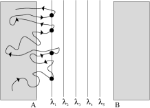
Figure 1: The first stage of the FFS method.

Figure 2 illustrates the next stage of the algorithm. The collection of points at $\lambda_{1}$ is used to initiate a large number $M_{1}$ of short simulation trial runs. In each of these trials, a phase space point from the collection at $\lambda_{1}$ is chosen at random. This is then used as the starting point for a simulation run, which is continued until the system crosses either $\lambda_{2}$ or $\lambda_{A}$. During this run, the maximum value of $\lambda$, $\lambda_{max}$, achieved by the system is recorded. Counters $N_{1}^{j}$ for all the sub-surfaces $\lambda_{1}^{(j)}\leq\lambda_{max}$ are then incremented by one. After $M_{1}$ trials, a good estimate is obtained for $P(\lambda_{1}^{(j)}|\lambda_{1})=N_{1}^{j}/M_{1}$, for $1\leq j\leq m_{1}$. We note that $P(\lambda_{1}^{(1)}|\lambda_{1})=1$ and $P(\lambda_{1}^{(m_{1})}|\lambda_{1})=P(\lambda_{2}|\lambda_{1})$.

During the trial procedure outlined above, one also makes a new collection of $C_{2}$ points at or just beyond the surface $\lambda_{2}$: these are the final phase space points of those trial runs starting from $\lambda_{1}$ which make it to $\lambda_{2}$. The number $M_{2}$ of trials must be large enough to generate $C_{2}$ points at $\lambda_{2}$. The values of $M_{2}$, $C_{2}$ and $M_{i}$ and $C_{i}$ for all the subsequent surfaces $2\leq i\leq n$ are chosen by the user: the $C_{i}$ should be large enough to allow good sampling of the phase space.

Figure 2: The second stage of the FFS method.

The trial run procedure is repeated for each subsequent surface $\lambda_{i}$, starting from the collection of $C_{i}$ phase space points generated by the successful runs from $\lambda_{i-1}$. Eventually $\lambda_{B}$ is reached, and one is left with a series of histograms $P(\lambda_{i+1}^{(j)}|\lambda_{i})$, for $1\leq i\leq n$ and $1<j\leq m_{i}$. Using equation (6), these histograms can be fitted together to obtain a smooth curve $P(\lambda|\lambda_{1})$ ferrenberg ; duijneveld , the value of which at $\lambda=\lambda_{B}$ is $P(\lambda_{B}|\lambda_{1})$. The rate constant $k_{AB}$ is obtained on multiplying $P(\lambda_{B}|\lambda_{1})$ by the flux ${\overline{\Phi}}_{A,1}/{\overline{h}}_{\mathcal{A}}$ calculated in the first stage of the algorithm.

It is important to remark that the FFS algorithm does not assume that the distribution of phase space points at the interfaces $\{\lambda_{1}\dots\lambda_{n}\}$ is equal to the stationary distribution of states. For the example which we present in this paper, this turns out to have significant consequences for the transition mechanism.

Application: A Genetic Switch

We have applied the FFS method to a simplified model of a genetic toggle switch warren1 ; kepler ; cherry . This model could be regarded as a minimal representation of the lysis-lysogeny switch in bacteriophage $\lambda$ ptashne ; a synthetic switch of this type has also been constructed in vivo gardner .

The model switch consists of two proteins $\mathrm{A}$ and $\mathrm{B}$ and their corresponding genes $A$ and $B$. $\mathrm{A}$ and $\mathrm{B}$ form homodimers $\mathrm{A}_{2}$ and $\mathrm{B}_{2}$ which can bind to the DNA strand (here labeled $\mathrm{O}$) and influence transcription. When the dimer $\mathrm{A}_{2}$ is bound to the DNA, gene $B$ is not transcribed, while $\mathrm{B}_{2}$, when bound, correspondingly blocks transcription of gene $A$: thus $\mathrm{A}$ and $\mathrm{B}$ mutually repress one another’s production. Both proteins are also degraded in the monomer form. We consider two versions of this switch: the “general” switch, in which both dimers can bind simultaneously to the DNA, forming the species $\mathrm{O}\mathrm{A}_{2}\mathrm{B}_{2}$, and the “exclusive” switch, in which only one dimer can be bound at any time. The exclusive switch models the case where the operator regions of genes $A$ and $B$ are overlapping.

The switch is represented by the set of reactions (7a).

$$2\mathrm{A}\rightleftharpoons\mathrm{A}_{2} 2\mathrm{B}\rightleftharpoons\mathrm{B}_{2}$$ (7a)

$$\mathrm{O}+\mathrm{A}_{2}\rightleftharpoons\mathrm{O}\mathrm{A}_{2} \mathrm{O}+\mathrm{B}_{2}\rightleftharpoons\mathrm{O}\mathrm{B}_{2}$$ (7b)

$$\mathrm{O}\mathrm{A}_{2}+\mathrm{B}_{2}\rightleftharpoons\mathrm{O}\mathrm{A}_{2}\mathrm{B}_{2} \,\,*\,\, \mathrm{O}\mathrm{B}_{2}+\mathrm{A}_{2}\rightleftharpoons\mathrm{O}\mathrm{A}_{2}\mathrm{B}_{2}\qquad$$ (7c)

$$\mathrm{O}\to\mathrm{O}+\mathrm{A} \mathrm{O}\to\mathrm{O}+\mathrm{B}$$ (7d)

$$\mathrm{O}\mathrm{A}_{2}\to\mathrm{O}\mathrm{A}_{2}+\mathrm{A} \mathrm{O}\mathrm{B}_{2}\to\mathrm{O}\mathrm{B}_{2}+\mathrm{B}$$ (7e)

$$\mathrm{A}\to\emptyset \mathrm{B}\to\emptyset$$ (7f)

The asterisk indicates that reaction (7c) happens only for the general switch. Here, we study a symmetrical version of the switch: the rate constants for the reactions on the left and right-hand sides of scheme (7a) are identical. These are all expressed in terms of the protein production rate constant $k$ (for reactions (7d) and (7e)), so that the unit of time in our calculations is $k^{-1}$. The rate constants for both the forward and backward dimerization reactions (7a) are $5k$. Binding to the DNA occurs with rate constant $5k$ and dissociation of the complex with rate constant $k$ (reactions (7b) and (7c)). Finally, the rate constant for protein degradation, reactions (7f), is $0.25k$. These parameters are chosen such that in a simulation using the Gillespie algorithm, the switch flips between the $\mathrm{A}$- and $\mathrm{B}$-rich states at a rate that can be measured by brute-force simulation. This allows us to test the FFS method. The model is, of course, highly simplistic: our aim is here to demonstrate the FFS scheme using a simple example.

Results

Figure 3 shows the results of Gillespie simulations of the model genetic switch, in the general (a) and exclusive (b) cases. The difference $\Delta$ in the total copy numbers of the two proteins, $\Delta=\mathrm{N_{B}}-\mathrm{N_{A}}$, is plotted as a function of time, where $\mathrm{N_{A}}$ and $\mathrm{N_{B}}$ are defined by:

$$\mathrm{N_{A}}=n_{\mathrm{A}}+2n_{\mathrm{A}_{2}}+2n_{\mathrm{O}\mathrm{A}_{2}}+2n_{\mathrm{O}\mathrm{A}_{2}\mathrm{B}_{2}}$$ (8)

$$\mathrm{N_{B}}=n_{\mathrm{B}}+2n_{\mathrm{B}_{2}}+2n_{\mathrm{O}\mathrm{B}_{2}}+2n_{\mathrm{O}\mathrm{A}_{2}\mathrm{B}_{2}}$$

Of course, $n_{\mathrm{O}\mathrm{A}_{2}\mathrm{B}_{2}}=0$ for the exclusive switch. Noting the different scales on the time axis, the exclusive switch (b) has a much lower flipping rate than the general switch (a), in agreement with previous work warren1 . The probability $P(\Delta)$ of obtaining a particular value of $\Delta$ is shown in the insets, demonstrating clearly that both the general and exclusive switches are bistable.

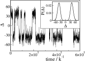
(a) (b)

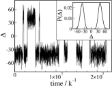
Figure 3: $\Delta$ as a function of time (in units of $k^{-1}$) for a typical simulation run, for the general (a) and exclusive (b) switches. Insets show probability $P(\Delta)$ of observing a particular value of $\Delta$, calculated over a total simulation time of $1\times 10^{7}k^{-1}$ (general switch, (a)) and $5\times 10^{9}k^{-1}$ (exclusive switch, (b)).

Using long brute-force Gillespie simulations, the rate constant for the transition from the $\mathrm{A}$-rich to the $\mathrm{B}$-rich state was obtained for each switch. We define phase space region $A$ to be where $\Delta\leq-25$, and region $B$ to be where $\Delta\geq 25$. The system flips stochastically between the state where $h_{\mathcal{A}}=1$ and $h_{\mathcal{B}}=0$ (i.e. it was most recently in $A$) and that where $h_{\mathcal{A}}=0$ and $h_{\mathcal{B}}=1$ (it was most recently in $B$). The times $t$ between flipping events are distributed according to a Poisson distribution $p(t)=k_{AB}\exp{[-k_{AB}t]}$, where $k_{AB}=k_{BA}$ since the switch is symmetrical in $A$ and $B$. The rate constant $k_{AB}$ can conveniently be measured by fitting the cumulative distribution $F(t)=\int_{0}^{t}dt^{\prime}\,p(t^{\prime})$ to the function $1-\exp{[-k_{AB}t]}$. This procedure resulted in values of $k_{AB}=(4.21\pm 0.05)\times 10^{-5}k$ for the general switch and $k_{AB}=(9.4\pm 0.2)\times 10^{-7}k$ for the exclusive switch (using simulation runs of total length $3\times 10^{8}k^{-1}$ [12546 flips observed] and $9\times 10^{9}k^{-1}$ [8808 flips observed] respectively).

We next re-calculated $k_{AB}$ using FFS. The surfaces $\{\lambda_{1}\dots\lambda_{n}\}$, were defined in terms of $\Delta$: i.e. $\lambda=\Delta$. Regions $A$ and $B$ are given by $\lambda=\Delta\leq\lambda_{A}$ and $\lambda=\Delta\geq\lambda_{B}$, respectively. To be sure that the exact values of $\lambda_{A}$, $\lambda_{B}$ and $\{\lambda_{1}\dots\lambda_{n}\}$ did not affect the result, these parameters were varied in a series of separate calculations. In all cases, we set $\lambda_{1}=\lambda_{A}$, and at each surface $\lambda_{i}$, $C_{i}=10000$ points were stored and $M_{i}=100000$ shooting trials were made. Results were averaged over $10$ independent calculations, to obtain error bars similar to those of the brute-force results.

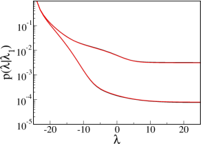
Figure 4: $P(\lambda|\lambda_{1})$ for the general (top) and exclusive (bottom) switches, where $\lambda_{A}=-24$ and $\lambda_{B}=25$. Black lines: brute-force simulation results (averaged over a total time $1\times 10^{8}k^{-1}$ for the general switch and $9\times 10^{9}k^{-1}$ for the exclusive switch); Red lines: FFS results, averaged over 10 independent calculations.

Figure 4 shows $P(\lambda|\lambda_{1})$ as a function of $\lambda$, for the general and exclusive switches. This function can also be obtained from an analysis of the brute-force simulation trajectories: the figure shows excellent agreement between the brute-force results (shown in black), and those of FFS (shown in red).

General switch
$\lambda_{B}$	$n$	$f/k\times 10^{-2}$	$P(\lambda_{B}|\lambda_{1})\times 10^{-3}$	$k_{AB}/k\times 10^{-5}$
$30$	$14$	$2.97\pm 0.01$	$1.41\pm 0.03$	$4.19\pm 0.07$
$25$	$11$	$1.33\pm 0.01$	$3.10\pm 0.06$	$4.11\pm 0.07$
$20$	$9$	$0.392\pm 0.003$	$10.5\pm 0.1$	$4.13\pm 0.04$
$\bf 25$	-	$\bf 1.339\pm 0.004$	$\bf 3.15\pm 0.05$	$\bf 4.22\pm 0.06$
				$\bf 4.21\pm 0.05$
Exclusive switch
$\lambda_{B}$	$n$	$f/k\times 10^{-2}$	$P(\lambda_{B}|\lambda_{1})\times 10^{-5}$	$k_{AB}/k\times 10^{-7}$
$30$	$16$	$2.98\pm 0.01$	$3.2\pm 0.1$	$9.5\pm 0.3$
$25$	$11$	$1.211\pm 0.007$	$7.8\pm 0.3$	$9.5\pm 0.3$
$20$	$10$	$0.282\pm 0.002$	$33.7\pm 0.8$	$9.6\pm 0.2$
$\bf 25$	-	$\bf 1.2112\pm 0.0004$	$\bf 7.70\pm 0.09$	$\bf 9.3\pm 0.1$
				$\bf 9.4\pm 0.2$

Table 1: Results for $f={\overline{\Phi}}_{A,1}/{\overline{h}}_{\mathcal{A}}$, $P(\lambda_{B}|\lambda_{1})$ and $k_{AB}$, for the general and exclusive switches. FFS results are averaged over 10 independent runs, using $n$ surfaces, as described in the text. Brute-force results, in bold type, are averaged over runs of length $3\times 10^{8}k^{-1}$ (general) and $9\times 10^{9}k^{-1}$ (exclusive). The upper value of $k_{AB}$ is calculated using equation (4) and the lower value using the fitting of $F(t)$ described in the text.

FFS			Brute-Force
	$\lambda_{B}$	CPU		CPU
general	$20$	$1.9$	general	$6.8$
general	$25$	$1.1$
general	$30$	$1.3$
exclusive	$20$	$2.1$	exclusive	$90.2$
exclusive	$25$	$1$
exclusive	$30$	$1.7$

Table 2: Relative CPU time required to calculate the values of $k_{AB}$ given in table 1, using parameter values as in the text. For the FFS calculations, the calculation of the flux $f={\overline{\Phi}}_{A,1}/{\overline{h}}_{\mathcal{A}}$ accounted for $20-40$% of the total CPU time.

Table 1 lists the results for $f={\overline{\Phi}}_{A,1}/{\overline{h}}_{\mathcal{A}}$ and $P(\lambda_{B}|\lambda_{1})$, as well as $k_{AB}$, for various choices of $\lambda_{A}$ and $\lambda_{B}$. The number $n$ of surfaces used in each calculation is also listed. In all cases, the rate constant $k_{AB}$ is in good agreement with the brute-force simulation result. An additional test is provided by measuring $f$ and $P(\lambda|\lambda_{1})$ using the brute-force runs, to provide a second brute-force estimate for $k_{AB}$. This value is also listed in table 1 and, as expected, is in good agreement both with the value obtained by the fitting to Poisson statistics, and with the FFS results.

Table 2 shows the relative CPU time required for each of the calculations. Even for the general switch with a relatively fast flipping rate, estimates of $k_{AB}$ are obtained by the FFS method $3-6$ times faster than using brute-force simulations, with similar accuracy. In the case of the exclusive switch, the FFS method is $40-90$ times more efficient. Table 2 also demonstrates that the CPU time required for an FFS calculation does not increase as the rate $k_{AB}$ decreases, in contrast to the time for brute-force calculations. Thus FFS should allow the calculation of rates of even very rare flipping events within reasonable computational time. As an example, we have calculated the rate of flipping for a more stable version of the exclusive switch, in which the rate constant for protein degradation is reduced to $0.175k$. Using the FFS method, we obtain a rate $k_{AB}=(1.92\pm 0.09)\times 10^{-9}k$, 500 times slower than the switch considered above. This result would have been extremely difficult to obtain using brute-force simulation.

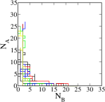
(a)   (b)

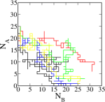
Figure 5: Five randomly chosen transition paths, plotted as a function of $\mathrm{N_{A}}$ and $\mathrm{N_{B}}$ (a): general switch (b): exclusive switch.

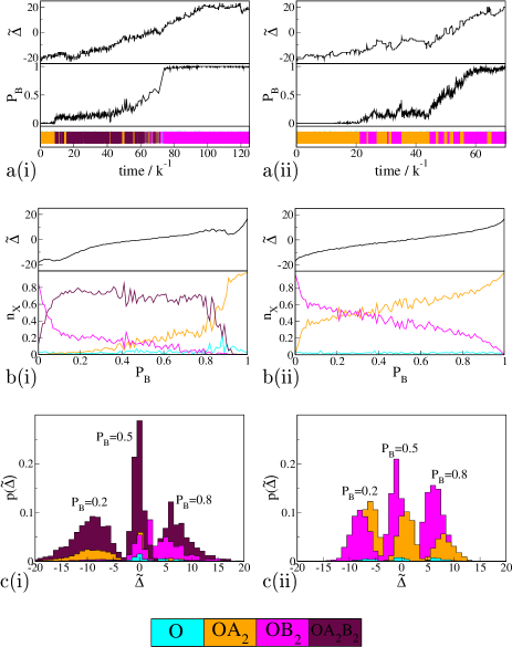
Figure 6: (a): Typical transition paths, for the general (i) and exclusive (ii) switches. $\tilde{\Delta}=(n_{\mathrm{B}}+2n_{\mathrm{B}_{2}})-(n_{\mathrm{A}}+2n_{\mathrm{A}_{2}})$, $P_{B}$ and operator occupancy (color-coded) are plotted versus time. The path for the general switch (a) happens to be longer than that for the exclusive switch (b), but this is not true of all paths in the ensemble. (b): Average values of ${\tilde{\Delta}}$ and average operator occupancies, as functions of the committor $P_{B}$, for the general (i) and exclusive (ii) switches. (c): Probability distribution $p(\tilde{\Delta})$, for selected values of $P_{B}$. $p(\tilde{\Delta})$ is divided into color-coded contributions from the different operator states. The sum of the areas of the histograms for a particular $P_{B}$ is unity. For all plots, $100$ test trajectories were used to estimate $P_{B}$.

The results presented in table 1 show that for the same mean number of protein molecules, the exclusive switch has a flipping rate approximately $50$ times slower than that of the general switch, in agreement with previous work warren1 . In order to elucidate the origin of this difference, we have analysed the flipping mechanism. The FFS method generates a collection of switching trajectories (members of the TPE). Figure 5 shows a sample of five of these transition paths, for the general switch (a) and the exclusive switch (b), plotted as a function of $\mathrm{N_{A}}$ and $\mathrm{N_{B}}$. To obtain these paths, we begin with the collection of partial trajectories that reach $\lambda_{B}$ from $\lambda_{n}$ and trace these back via the intervening surfaces to $\lambda_{A}$. It is clear from figure 5 that in the general switch, protein $\mathrm{A}$ is lost before protein $\mathrm{B}$ is gained, so that the transition passes through a region of phase space where both $\mathrm{N_{A}}$ and $\mathrm{N_{B}}$ are low. However, this is not the case for the exclusive switch. An important quantity associated with transition paths is the committor, $P_{B}(X)$. This is the probability that a new simulation trajectory fired from point $x$ will reach region $B$ before $A$ tps . We have measured $P_{B}(x)$ for points along the trajectories in the transition path ensembles generated using FFS, for the general and exclusive switches. Figure 6(a) shows $P_{B}$, as well as $\tilde{\Delta}=(n_{\mathrm{B}}+2n_{\mathrm{B}_{2}})-(n_{\mathrm{A}}+2n_{\mathrm{A}_{2}})$ and the occupancy of the operator sites, as functions of time for typical transition paths. ${\tilde{\Delta}}$ measures the difference in the number of free protein molecules: it is similar but not identical to $\Delta$. A key point is that for the general switch (figure 6a(i)), the operator makes two important changes of state, from ${\mathrm{OA}}_{2}$ to ${\mathrm{OA}}_{2}{\mathrm{B}}_{2}$ early in the transition process, and later from ${\mathrm{OA}}_{2}{\mathrm{B}}_{2}$ to ${\mathrm{OB}}_{2}$. Both of these changes influence $P_{B}$. For the exclusive switch (figure 6a(ii)), however, the operator is intermittently in states ${\mathrm{OA}}_{2}$ and ${\mathrm{OB}}_{2}$ during the transition.

In figure 6 (b), values of ${\tilde{\Delta}}$ and operator occupancies are shown, averaged over the paths in the TPE, as a function of the committor $P_{B}$. Results are shown for the general (i) and exclusive (ii) switches. Figure 6 (c) analyses the state points along the paths in the TPE which have values of $P_{B}=0.2$, $P_{B}=0.5$ and $P_{B}=0.8$. For each of these values of the committor, points are grouped according to their operator state. For each $P_{B}$ and operator state, the histograms in figure 6(c) show the probability distribution function $p({\tilde{\Delta}})$. Clearly, for points on a constant $P_{B}$ surface, the operator state and the number of free molecules are correlated: when $\mathrm{A}$ is bound to the DNA, on average, a larger $\tilde{\Delta}$ is required to obtain a particular value of $P_{B}$ than when $\mathrm{B}$ is bound. This shows that $P_{B}$, and hence the reaction co-ordinate, depends not only upon the difference in copy number $\tilde{\Delta}$, but also on the state of the operator. Importantly, the plots of figure 6 (b) and (c) are not symmetric on making the transformations $P_{B}\to 1-P_{B}$, ${\tilde{\Delta}}\to-{\tilde{\Delta}}$ and $\mathrm{O}\mathrm{A}_{2}\leftrightarrow\mathrm{O}\mathrm{B}_{2}$. This demonstrates that the distribution of transition paths does not follow the steady state phase space density, which is symmetric on interchanging $\mathrm{A}$ and $\mathrm{B}$, since the switch is by construction symmetric tenwolde . It also means that the TPE for the reverse transition, from $B$ to $A$, would occupy a different region of phase space, as compared to the TPE for the transition from $A$ to $B$ (see also supplementary material). The origin of this asymmetry is that the dynamics of our system involves irreversible reactions (Reactions (7d-7f)). Indeed, our system does not satisfy microscopic reversibility. Finally, figure 6 clearly demonstrates why the elimination of the operator state $\mathrm{O}\mathrm{A}_{2}\mathrm{B}_{2}$ for the exclusive switches enhances its stability with respect to that of the general switch. In the general switch, as soon as a $\mathrm{B}_{2}$ dimer is produced by some rare fluctuation, it can bind to the DNA, switch off the production of $\mathrm{A}$ and thereby accelerate the flipping of the switch. For the exclusive switch, however, any $\mathrm{B}_{2}$ dimer that is produced must wait for a second fluctuation by which $\mathrm{A}_{2}$ is released from the DNA, before it can bind. This is the origin of the enhanced stability of the exclusive switch.

Discussion

This article presents the Forward Flux Sampling (FFS) method for the calculation of the rates of rare events in stochastic kinetic simulation schemes such as those used for biochemical reaction networks. In contrast to previously developed methods for sampling the transition path ensemble tps ; vanerp , FFS does not require knowledge of the phase space density. It is this feature that makes it possible to study rare events in biochemical networks. Our algorithm samples the TPE in a way that is, to our knowledge, new: many paths are grown simultaneously from state $A$ to state $B$ in a series of layers of partial paths, each layer forming the basis for the next. The phase space separating stable states $A$ and $B$ is traversed by the algorithm in a “ratchet-like” manner, making the method highly suitable for very rare events, where one-at-a-time path generation tends to be inefficient. FFS is not applicable to systems whose dynamics is deterministic. It could be used, however, in combination with any stochastic simulation technique. This will make it useful for a wide range of problems in soft condensed matter systems, including rare events and non-equilibrium processes.

We have demonstrated our method using stochastic simulations of a simple genetic switch consisting of two mutually repressing genes. Following earlier work warren1 , we compare the case where both protein products can bind simultaneously as dimers to the DNA (the general switch), to that where each protein dimer excludes the binding of the other (the exclusive switch). The results obtained using FFS are in good agreement with those of long brute-force simulations for both switches. The computational time required for the FFS calculations is far less than for the brute-force simulations, and in addition, does not increase as the rate constant decreases. Indeed, using FFS we could simulate a switch that was too stable to be studied using brute-force calculations. By analysing the transition path ensembles we were able to discover the differences between the flipping mechanisms for the general and exclusive switches. These allow us to understand the origin of the enhanced stability of the exclusive switch. The FFS method will be easily applicable to many important biochemical switches, for which prediction of the rates and pathways of switching should lead to a better understanding of the design principles underlying their stability.

We thank Peter Bolhuis for very helpful discussions and Daan Frenkel, Rutger Hermsen and Harald Tepper for their careful reading of the manuscript. The work is part of the research program of the “Stichting voor Fundamenteel Onderzoek der Materie (FOM)”, which is financially supported by the “Nederlandse organisatie voor Wetenschappelijk Onderzoek (NWO)”.

References

- (1) Ptashne, M. (1986) (Cell Press & Blackwell Scientific Publications ).
- (2) Müller-Hill, B. (1996) The Lac Operon: A Short History of a Genetic Paradigm (Walter de Gruyter, Berlin).
- (3) Ozbudak, E. M., Thattai, M., Lim, H. N., Shraiman, B. I., & van Oudenaarden, A. (2004) Nature 427, 737–740.
- (4) Vilar, J. M. G., Guet, C. C., & Leibler, S. (2003) J. Cell. Biol. 161, 471–476.
- (5) Pomerening, J. R., Sontag, E. D., & Ferrell, J. E., Jr. (2003) Nature Cell Biol. 5, 346–351.
- (6) Sha, W., Moore, J., Chen, K., Lassaletta, A. D., Yi, C.-S., Tyson, J. J., & Sible, J. C. (2003) Proc. Natl. Acad. Sci. USA 100, 975–980.
- (7) Ferrell, J. E., Jr. & Machleder, E. M. (1998) Science 280, 895–898.
- (8) Xiong, W. & Ferrell, J. E., Jr. (2003) Nature 426, 460–465.
- (9) Angeli, D., Ferrell, J. E., Jr., & Sontag, E. D. (2004) Proc. Natl. Acad. Sci. USA 101, 1822–1827.
- (10) Ferrell, J. E., Jr. (2002) Curr. Opin. Cell. Biol. 14, 140–148.
- (11) Gardner, T. S., Cantor, C. R., & Collins, J. J. (2000) Nature 403, 339–342.
- (12) Atkinson, M. R., Savageau, M. A., Myers, J. T., & Ninfa, A. J. (2003) Cell 113, 597–607.
- (13) Becskei, A., Séraphin, B., & Serrano, L. (2001) EMBO J. 20, 2528–2535.
- (14) van Kampen, N. G. (1992) Stochastic Processes in Physics and Chemistry (North-Holland, Amsterdam).
- (15) Gardiner, C. W. (1985) Handbook of Stochastic Methods (Springer-Verlag, Berlin), Second edition.
- (16) Gillespie, D. T. (1976) J. Comput. Phys. 22, 403–434.
- (17) Gillespie, D. T. (1977) J. Phys. Chem. 81, 2340–2361.
- (18) Morton-Firth, C. J. & Bray, D. (1998) J. Theor. Biol. 192, 117–128.
- (19) van Zon, J. S. & ten Wolde, P. R. (2004), q-bio.MN/0404002.
- (20) Aurell, E. & Sneppen, K. (2002) Phys. Rev. Lett. 88, 048101 1–4.
- (21) Aurell, E., Brown, S., Johanson, J., & Sneppen, K. (2002) Phys. Rev. E 65, 051914 1–9.
- (22) Frenkel, D. & Smit, B. (2002) Understanding Molecular Simulation. From Algorithms to Applications (Academic Press, Boston), Second edition.
- (23) Dellago, C., Bolhuis, P. G., Csajka, F. S., & Chandler, D. (1998) J. Chem. Phys. 108, 1964–1977.
- (24) Dellago, C., Bolhuis, P. G., & Geissler, P. L. (2002) Adv. Chem. Phys. 123, 1–78.
- (25) Bolhuis, P. G., Chandler, D., Dellago, C., & Geissler, P. L. (2002) Annu. Rev. Phys. Chem. 53, 291–318.
- (26) Warren, P. B. & ten Wolde, P. R. (2004) Phys. Rev. Lett. 92, 128101 1–4.
- (27) Newman, M. E. J. & Barkema, G. T. (1999) Monte Carlo Methods in Statistical Physics (Oxford University Press, Oxford).
- (28) Bortz, A. B., Kalos, M. H., & Lebowitz, J. L. (1975) J. Comp. Phys. 17, 10–31.
- (29) Reichl, L. E. (1998) A Modern Course in Statistical Physics (John Wiley and Sons, Inc., New York), Second edition.
- (30) van Erp, T. S., Moroni, D., & Bolhuis, P. G. (2003) J. Chem. Phys. 118, 7762.
- (31) Ferrenberg, A. M. & Swendsen, R. H. (1989) Phys. Rev. Lett. 63, 1195–1198.
- (32) van Duijneveldt, J. S. & Frenkel, D. (1992) J. Chem. Phys. 96, 4655–4668.
- (33) Kepler, T. B. & Elston, T. C. (2001) Biophys. J. 81, 3116–3136.
- (34) Cherry, J. L. & Adler, F. R. (2000) J. Theor. Biol. 203, 117–133.
- (35) ten Wolde, P. R. & Chandler, D. (2002) Proc. Natl. Acad. Sci. USA 99, 6539–6543.