Subthreshold oscillations in a map-based neuron model

Abstract

Self-sustained subthreshold oscillations in a discrete-time model of neuronal behavior are considered. We discuss bifurcation scenarios explaining the birth of these oscillations and their transformation into tonic spikes. Specific features of these transitions caused by the discrete-time dynamics of the model and the influence of external noise are discussed.

1 Introduction

Studies of dynamical behavior of biological networks require numerical simulations of arrays containing a very large number of neurons. Despite the variety of physiological processes involved in the formation of neuron activity, the thorough studies of the large-scale networks need simple phenomenological models that can replicate the dynamics of individual neurons. Various suggestions for the design of low-dimensional maps for modeling the neurons’ behavior have been proposed, see for example [1, 2, 3, 4, 5, 6] and references therein. Most of them were focused on the replication of either fast spikes or relatively slow bursts while the mechanisms for generation of specific footprints of spikes were neglected.

A simple discrete-time model replicating the spiking-bursting neural activity has been suggested recently in [7]. This model is a 2D map that mimics rather realistically various types of transitions that occur in biological neurons. These transitions include routes between silence and tonic spiking as well as a triplet: silence $\leftrightarrow$ bursts of spikes $\leftrightarrow$ tonic spiking. Such simple phenomenological models bear a high potential for further developments of computationally efficient methods for studies of functional behavior in large-scale neurobiological networks [8].

The bifurcation analysis of the map model carried out in [9] has shown that the transition from silence (a stable fixed point) to generation of action potentials is characterized by a sub-critical Andronov-Hopf bifurcation when an unstable invariant closed curve collapses into the stable fixed point. Therefore, the original map-model [7] provides only an abrupt transition from silence to spiking as a control parameter (e.g. the depolarization current) passes the excitability threshold. This scenario is quite typical for most types of biological neurons. However, experimental studies suggest that some neurons may come out of the silence softly through the regime of small oscillations below the threshold of the spike excitation [10]. These subthreshold oscillations of almost sinusoidal form facilitate the generation of spike oscillations when the membrane gets depolarized or hyperpolarized [11, 12]. These small oscillations can play an important role in shaping specific forms of rhythmic activity that are vulnerable to the noise in the network dynamics [15, 16].

In this paper we modify the map model so that it can generate stable subthreshold oscillations. We start the discussion of the model dynamics with the analysis of local bifurcations of a fixed point of the map. We show that the loss of stability of the fixed point is accompanied by the birth of the stable invariant circle which initiate a family of canards in the map. Further evolution of the circle leads to a breakdown of the invariant circle that gives rise to chaos. We also elaborate on the mechanism of the onset of irregular spiking which is due to heteroclinic-like crossings between the stable and unstable invariant sets, which are the images of the slow motion “surfaces” in the unperturbed map. The role played by small subthreshold oscillations in the responsiveness of the map to external noise is considered.

2 Map-based model with stable subthreshold oscillations

The map-based model of spiking-bursting neuron oscillations, following [7], can be written in the form of the two-dimensional map

$$\bar{x} = f_{\alpha}(x,y+\beta),$$ (1a)

$$\bar{y} = y-\mu(x+1-\sigma),$$ (1b)

where the $x$-variable replicates the dynamics of the membrane potential, the parameters $\alpha$, $\sigma$ and $0<\mu\ll 1$ control individual dynamics of the system. Some input parameters $\beta$ and $\sigma$ are employed to provide coupling with other such models afterwards; both stand for injected currents. The principal distinction of the original map analyzed in [7, 9] and the one in question is camouflaged in the function $f_{\alpha}(x,y+\beta)$, which is given by

$$f_{\alpha}(x,y+\beta)=\left\{\begin{array}[]{ll}-\alpha^{2}/4-\alpha+y+\beta,&x<-1-\alpha/2,\\ \alpha x+(x+1)^{2}+y+\beta,&-1-\alpha/2\leq x\leq 0,\\ y+1+\beta,&0<x<y+1+\beta,\\ -1,&x\geq y+1+\beta.\end{array}\right.$$ (6)

The graph of this function is pictured in Fig. 1. The shape of nonlinear function is meant to achieve a replication of sharp tonic spikes in the dynamics of the $x$-variable in the map. The slow $y$-variable can turn the spike generator on and off. The main difference between the function (2) and that in the map proposed in [7] is its shape on the left hand side of the discontinuity point, i.e. at $x<y+1+\beta$. Now the function contains an interval of parabola instead of a hyperbola used in [7, 9]. This modification is crucial for stability of subthreshold oscillations. The parabola reaches its minimum at $x=-1-\alpha/2$. At this point the graph of the function is continued leftward by a horizontal line, see Fig. 1.

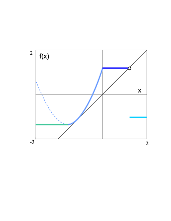
Figure 1: Geometry of the fast subsystem, map (1a), for the parameter values at the tangent bifurcation: $\alpha=1$ and $y=0$. The function is discontinuous at the point $x=y+1+\beta$ which belongs to the rightmost interval, see (2).

2.1 Fast and slow motions of the map

For map (1), when $\mu=0$, the slow subsystem (1b) is decoupled from the fast subsystem (1a), in which $y$ is regarded as a perturbation parameter. One may see from Fig. 1 that depending on $y$, the fast subsystem may have two fixed points, one stable and one unstable, or no fixed points. The transition between these states occurs via a saddle-node bifurcation. When $y$ is varied, the fixed points trace out a parabola in the $(y,x)$-plane as shown in Fig. 2. The traces of stable and unstable fixed points form on the $(x,y)$ stable, $S_{ps}$, and unstable, $S_{pu}$, branches, respectively.

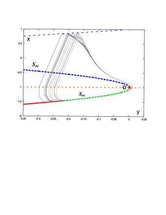
Figure 2: $(y,x)$-bifurcation diagram of the fast subsystem, map (1a), for $\alpha=1$ and $\mu=0$. The branches $S_{pu}$ and $S_{ps}$ are traced out by the stable and unstable fixed points of the fast map as the parameter $y$ varies. When $0<\mu\ll 1$, this $(y,x)$ plane becomes the phase portrait of the 2D map. The shown trajectory of the 2D map is computed at $\mu=0.04$, $\alpha=0.99$ and $\sigma=0$. The dashed curves are the zero level ones for function (2).

The point of intersection of these branches with the nullcline of slow subsystem (1b), which is given by $x_{fp}=\sigma-1$, is a fixed point of the two-dimensional map (1). It is easy to see that this fixed point $O$ is stable if it is located on $S_{ps}$ and is unstable if it is on $S_{pu}$. The case where the nullcline crosses the parabola at the fold point requires a more delicate analysis.

The nonstandard analysis [17] predicts that when $0<\mu\ll 1$, the normally hyperbolic branches $S_{ps}$ and $S_{ps}$ persist in the form of the stable and unstable “slow motion” sets ${\cal S}_{s}$ and ${\cal S}_{u}$ that remain $\mu$-close to the originals, but $\mu^{3/2}$-close to them near the fold [18].

The idea behind generation of tonic spikes in the map (1) is illustrated in Fig. 2. The period of spiking is comprised of the following phases: the rest phase, where the phase point slides along the set ${\cal S}_{s}$ at a rate of order $\mu$ towards the fold point. Then, the phase point jumps up indicating the beginning of a spike. Its upward motion is stopped by a delimiter (the third segment of function (2)) that reflects the phase point towards the stable slow surface ${\cal S}_{s}$ through the line segment $x=-1$.

2.2 Birth of invariant curve

Next we carry out the bifurcation analysis of the fixed point $O$. Our consideration is restricted to the domain $\alpha^{2}/2-\alpha+y+\beta\leq x<0$, i.e. to the parabolic segment of function (2). This means that the fast subsystem (1a) is chosen to be close to the tangent bifurcation. The moment of the bifurcation is pictured in Fig. 1. From (1b) one finds the $x$-coordinate of the fixed point $x_{fp}=\sigma-1$. Therefore, the fixed point is located at the parabolic segment of function when the parameter values are within the range $-\alpha/2<\sigma<1$. The $y$-coordinate of the fixed point for this range of parameters is $y_{fp}=(\sigma-1)(1-a)-\sigma^{2}-\beta$.

Since fixed point $O$ is a single fixed point of map (1), the further stability analysis is reduced to two possible local bifurcations: a flip where one of the multipliers of the fixed point equals $-1$; and the Andronov-Hopf bifurcation, where the fixed point possesses a pair of multipliers equal $e^{\pm i\varphi}$ on the unit circle. Simple calculations reveal that the flip bifurcation takes place outside of the considered parameter region.

In the case of the Andronov-Hopf (AH) bifurcation, the Jacobian

$$\bf J=\left[\begin{array}[]{cc}\alpha+2\sigma&1\\ -\mu&1\end{array}\right]$$

of the map equals $1$ at the fixed point, while its trace equals $2\cos\varphi$. The equation of the corresponding bifurcation curve $AH$ is given by

$$\alpha_{AH}=-2\sigma+1-\mu.$$ (7)

On this curve, the fixed point has a pair of complex conjugate multipliers:

$$\rho_{1,2}=1-\frac{\mu}{2}\pm\frac{i}{2}\sqrt{\mu(4-\mu)}=\cos\psi\pm i\sin\psi.$$ (8)

To determine the stability of fixed point $O$ right at the bifurcation state we need to evaluate the sign of the first Lyapunov coefficient $L_{1}$. Note that the value of $L_{1}$ is not an invariant as it depends on coordinate transformations. The critical fixed point $O$ is stable if $L_{1}<0$, and unstable if $L_{1}>0$.

Figure 3: Bifurcation diagram illustrating the birth of “small” subthreshold oscillations transforming into spikes as parameter $\sigma$ increases. Top and bottom branches corresponds to the highest and lowest values of the $x$-variable for a given value of parameter $\sigma$. The other parameters of the map are set as follows $\alpha=0.99$, $\beta=0.0$ and $\mu=0.02$.

Let us introduce new coordinates in which the fixed point is translated to the origin:

$$\left(\begin{array}[]{c}x\\ y\end{array}\right)\mapsto\left(\begin{array}[]{cc}x+1-\sigma\\ y+(\sigma-1)(\alpha-1)+\sigma^{2}+\beta\end{array}\right).$$

Now the map looks as follows

$$\bar{x}=(1-\mu)x+x^{2}+y,\qquad\bar{y}=y-\mu x.$$ (9)

Let us next make another transformation

$$\left(\begin{array}[]{c}x\\ y\end{array}\right)\mapsto\left(\begin{array}[]{cc}0&1\\ \sin\psi&1-\cos\psi\end{array}\right)\left(\begin{array}[]{c}\xi\\ \eta\end{array}\right),$$

with $\sin\psi$ and $\cos\psi$ defined in (8). This makes the linear part of (9) a rotation through $\psi$:

$$\left(\begin{array}[]{c}\bar{\xi}\\ \bar{\eta}\end{array}\right)=\left(\begin{array}[]{cr}\cos\psi&-\sin\psi,\\ \sin\psi&\cos\psi,\end{array}\right)\left(\begin{array}[]{c}\xi\\ \eta\end{array}\right)+\left(\begin{array}[]{c}\frac{\cos\psi-1}{\sin\psi}\\ 1\end{array}\right)\eta^{2}.$$

In variable $z=\xi+i\eta$ the map assumes the complex form

$$\bar{z}=ze^{i\psi}+\frac{c_{20}}{2}z^{2}+c_{11}zz^{*}+\frac{c_{02}}{2}{z^{*}}^{2}$$ (10)

with

$$c_{20}=\frac{1}{2}\left(\tan\frac{\psi}{2}-i\right),\quad c_{11}=\frac{1}{2}\left(i-\tan\frac{\psi}{2}\right),\quad c_{02}=\frac{1}{2}\left(\tan\frac{\psi}{2}-i\right).$$ (11)

The normalizing transformation

$$z\mapsto z-\frac{c_{20}}{e^{2i\psi}-e^{i\psi}}z^{2}-\frac{c_{11}}{1-e^{i\psi}}zz^{*}-\frac{c_{02}}{e^{-2i\psi}-e^{i\psi}}{z^{*}}^{2}$$

eliminates all the quadratic terms in (10) so that the coefficient $L_{1}$ at the desired cubic term in the resulting normal form

$$\bar{z}=e^{i\psi}z(1+(L_{1}+iS_{1})zz^{*})+O(\|z\|^{3})$$

becomes the sought Lyapunov value. Its expression reads as follows:

$$L_{1}=-{\mbox{Re}}\frac{(1-2e^{i\psi})e^{-2i\psi}c_{20}c_{11}}{2(1-e^{i\psi})}-\frac{|c_{11}|^{2}}{2}-\frac{|c_{02}|^{2}}{4}.$$ (12)

Substituting (11) into (12) yields

$$L_{1}=-\frac{1}{4}\frac{\cos(\psi)}{\cos(\psi)+1}=-\frac{2-\mu}{4(4-\mu)}<0$$

for all small $\mu$. Thus, the loss of stability of fixed point $O$ on the Andronov-Hopf bifurcation curve is accompanied by the birth of a stable closed invariant curve emerging from $O$. This mechanism of the birth of subthreshold periodic oscillations is illustrated in Fig. 3 as the parameter $\sigma$ increases.

Figure 4: Four waveforms of iterates $x_{n}$ versus the discrete time $n$ show the influence of an external Gaussian white noise with standard deviation $s$ on the map oscillations. The control parameters of the map are $\alpha=0.99$, $\sigma=-0.0001$ and $\mu=0.02$.

Figure 5: Histograms of the interspike interval (ISI) distribution computed for the waveforms shown in Fig. 4. (a) - $s=0.0002$; (b) - $s=0.002$ and (c) - $s=0.02$.

2.3 Noise and subthreshold oscillations

It was observed recently that subthreshold periodic activity shapes stochastic properties of spiking in a neuron influenced by noise, see for example [13, 14, 15, 16, 19, 20]. To illustrate similar properties in our model let us now consider the regime of subthreshold oscillations in the map with the presence of noise. For the sake of briefness we consider only the case when noise is applied to the fast subsystem. The discussion of the effects of noise, occurring in the fast and slow subsystems, can be found elsewhere [21, 22]. The system (1) in presence of noise can be written as follows

$$x_{n+1} = f_{\alpha}(x_{n},y_{n}+\beta)+\zeta_{n},$$ (13)

$$y_{n+1} = y_{n}-\mu(x_{n}+1-\sigma),$$ (14)

where $\zeta_{n}$ is a delta-correlated Gaussian White Noise (GWN) with zero mean value and standard deviation value $s$.

Waveforms of map model (1) operating in the regime of subthreshold oscillations and the influence of noise are shown in Fig. 4. Four traces plotted in the figure correspond to different values of the standard deviation, $s$, of GWN. The top trace presents the case where the level of noise is insufficient to induce an action potential (a spike). When the level of noise exceeds a critical level the map starts producing occasional spikes. Such spikes are more likely to occur at the top of oscillation. This behavior results in the formation of a multi-hump structure in the probability distribution function of interspike intervals (ISIs), see histograms shown in Fig. 5(a,b).

A further raise of the noise level increases the probability of the action potentials. As the result, spikes occur almost every period of the subthreshold oscillation (see the bottom trace in Fig. 4) and the distribution of probability density of ISIs transforms into a single hump structure, see Fig. 5(c). These results are in good agreement with the results obtained from ODE based neuron models [19, 20].

3 Tangles of critical curves and chaos

In the numerical simulations of map (1) we found that subthreshold oscillations may be interrupted by irregular spiking even in the absence of external noise. An example of such a behavior is presented in Fig. 6. This intermediate dynamics is observed only within a rather thin parameter interval at the border between the regimes of continuous subthreshold oscillations and tonic spike generation. To understand the dynamical mechanisms behind this sporadic spiking we numerically studied the evolution of an invariant circle as the parameter values enter this thin region.

Figure 6: Sporadic spiking in the map (1) computed with $a=1.25$, $\sigma=-0.13$ and $\mu=0.02$. The phase portrait of these oscillations is shown in Fig. 7(a).

It follows from the theory of canards that the parameter domain for the existence of a stable invariant circle is a narrow strip of the order of $O(\mu)$ that adjoins the bifurcation curve $AH$. Furthermore, the size of the circle increases abnormally fast as the parameter values deviate from the Andronov-Hopf bifurcation curve and approach the critical values where the invariant circle breaks down. Such extreme sensitivity to slight parameter deviations hamper the detailed analysis of bifurcations associated with the circle as it breaks.

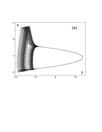
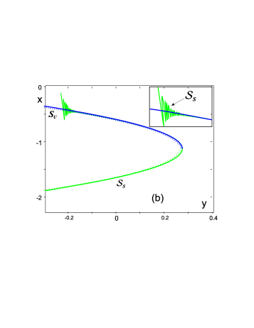
Figure 7: (a) Chaos in the noiseless map (1) computed with $\alpha=1.25$, $\sigma=-0.13$ and $\mu=0.02$ The corresponding waveform is shown in fig. 6. (b) Forward iterates of a small interval of the stable critical set ${\cal S}_{s}$ reveal increasing wiggles occurred around the unstable critical set ${\cal S}_{u}$.

The breakdown of the stable invariant circle leads to an interesting situation depicted in Fig. 7(a). One can observe the co-existence of two kinds of special solutions following the unstable slow branch ${\cal S}_{u}$. They are called canards with a head (a spike) and ones without it [17]. A canard is characterized by a growing level of exponential instability with respect to nearby solutions. This instability is a necessary first component of chaotic behavior observed in a system. In addition, the presence of two types of canards creates mixing and uncertainty, which is the second important ingredient for the onset of chaos. This type of chaos in the neuron model (1) appears as small subthreshold oscillations alternating with sporadic spikes, see Fig. 6.

To understand the dynamical mechanism behind the splitting of canards into two types, we conducted a numerical analysis of the behavior of ${\cal S}_{s}$ and ${\cal S}_{u}$ for various parameter values selected close to the threshold for the breakdown of the stable invariant circle. To plot ${\cal S}_{s}$, we iterated forward a large number of phase points initiated from a relatively short interval on the stable branch $S_{s}$, chosen as an initial approximation. Figure 7(b) shows how the connected forward images of this interval become non-smooth, generating growing wiggles around the unstable set ${\cal S}_{u}$. Note that the unstable set ${\cal S}_{s}$ is easily computed using inverse mapping , see Appendix A. The insert in Fig. 7(b) shows the zoomed-in wiggles. One can see from Fig. 7 (a) and (b) that upon entering the wiggling area, the phase point can land back in the stable set ${\cal S}_{s}$, thereby completing another round of subthreshold oscillations, or jump up to make a spike. Such a situation is referred to as dynamical uncertainty [25]. Loosely speaking, the place on ${\cal S}_{u}$ where the wiggles become noticeable indicates the threshold beyond which the behavior of the map becomes uncontrollable.

This situation is similar to the case of a periodically driven pendulum near a homoclinic orbit associated with the saddle point at the top. Such a system is typically studied using a Poincaré return mapping defined over the period of the external force. Under proper conditions, the saddle fixed point of the mapping will possess transversal crossings between its stable and unstable sets (formerly, the stable and unstable separatrices of the saddle equilibrium in the autonomous system). These crossings generate the Smale horseshoe and, therefore, symbolic shift-dynamics in the system, see details in [17, 23, 24] and references therein. By construction, this type of Poincareé mapping is a diffeomorphism. However, our map (2) is an endomorphism, e.g. a non-invertible one, and as a result it may possess some exotic features prohibited in the invertible maps, see more in [23]. One of those features is that the set ${\cal S}_{s}$ may self-cross (so does the set ${\cal S}_{u}$ in the backward time). This situation is sketched in Fig. 8(a) and also can be seen on the trajectories’ behavior in the lower left corner of the attractor shown in Fig. 7(a). One can assume that these self-crossings can stimulate the conditions for the onset of a topological Small horseshoe (see Fig. 8(b)), whose presence is a de-facto proof of complex chaotic dynamics.

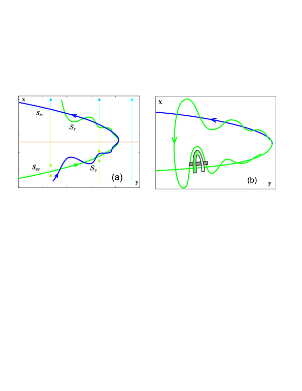
Figure 8: Heteroclinic-like crossings of the critical sets ${\cal S}^{s}$ and ${\cal S}^{u}$. Self-crossings of the set ${\cal S}^{s}$, which are one of the features of noninvertible maps, may generate a topological Smale horseshoe.

4 Conclusion

It is shown that a simple map can be employed to replicate the behavior of neurons with self-sustained subthreshold oscillations. These oscillations are achieved by a special selection of a nonlinear function in the fast subsystem. The dynamical mechanisms behind the transitions from silence to subthreshold oscillations of small amplitude and then to spiking activity are explained using the bifurcation approach.

Here we focused mostly on the individual dynamics of the map-based model. As a result we considered only the case when $\beta$ and $\sigma$ are constants. One may notice from (1) that the parameter $\beta$ can be eliminated by using the variable transformation $y+\beta\mapsto y$. However, the role of input parameter $\beta$ becomes important when a time dependant input is considered, see [7] for detail. We would like to note that for studies of non-autonomous dynamics of this map model one needs to modify function (2) to insure that no trajectory of (1) gets locked in the interval $0<x<y+1+\beta$ as $\beta$ or $y$ increase. The discussion on suggested alterations of the function to resolve this problem can be found elsewhere [7].

5 Acknowledgment

N.R. was supported in part by U.S. Department of Energy (grant DE-FG03-95ER14516). A.S. acknowledges the RFBR grants No. 02-01-00273 and No. 01-01-00975.

6 Appendix: Inverse map

To locate the unstable set ${\cal S}^{u}$ which is a surface of slow motion one should consider the inverse map $F_{inv}:(x,y)\mapsto(\bar{x},\bar{y})\in D$ defined in $D:=\,\{-1-\alpha/2\leq x\leq 0\}$. Within $D$ the inverse $F_{inv}$ assumes the following form

$$\bar{x} = \alpha x+(x+1)^{2}+y+\beta,$$ (15a)

$$\bar{y} = y-\mu(x+1-\sigma).$$ (15b)

Subtracting (15b) from (15a) one gets

$$\bar{x}-\bar{y}=\alpha x+(x+1)^{2}+\mu(x+1-\sigma)+\beta.$$ (16)

Solving it for $x$ one can find $x$ as a the following function in $\bar{x}$ and $\bar{y}$

$$x=-(2+\alpha+\mu)/2+\sqrt{(2+\alpha+\mu)^{2}/4-(1+\beta+\mu(1-\sigma)-\bar{x}+\bar{y}}.$$ (17)

To get the equation for the $y$-variable expression (17) must be plugged into (15b).

References

- [1] D.R. Chialvo and A.V. Apkarian, J. Stat. Phys. 70, 375 (1993).
- [2] D.R. Chialvo, Chaos, Solitons and Fractals 5, 461 (1995).
- [3] B. Cazelles, M. Courbage, and M. Rabinovich, Europhys. Lett. 56, 504 (2001).
- [4] N.F. Rulkov, Phys. Rev. Lett. 86, 183 (2001)
- [5] K.V. Andreev and L.V. Krasichkov Izv. Akad. Nauk Fiz. 66, 1777 (2002).
- [6] E.M. Izhikevich and F.C. Hoppensteadt, Bursting Mappings, submitted for publication. 2003
- [7] N.F. Rulkov, Phys. Rev. E 65, 041922 (2002).
- [8] N. F. Rulkov, M.V. Bazhenov, and A. L. Shilnikov, Proceedings of International Symposium on Topical Problems of Nonlinear Wave Physics, Russia, September 2003.
- [9] A. L. Shilnikov and N.F. Rulkov, Int. J. Bif. Chaos 13, 11 (2003).
- [10] R. Llinás, Science 242, 1654 (1988).
- [11] R. Llinás and Y. Yarom, Journal of Physiology 315, 549 (1981).
- [12] R. Llinás and Y. Yarom, Journal of Physiology 376, 163 (1986).
- [13] H.A. Braun, H. Wissing, K. Schäfer, M.C. Hirsch, Nature 367270 (1994).
- [14] M. Heinz, K. Schäfer, H.A. Braun, Brain Res 521 289, (1990).
- [15] V.A. Makarov, V.I. Nekorkin, and M.G. Velarde, Phys. Rev. Lett. 86, 3431 (2001).
- [16] M.G. Velarde, V.I. Nekorkin, V.B. Kazantsev, V.I. Makarenko, and R. Llinás, Neural Networks 15 5 (2002).
- [17] V. I. Arnold, V.S. Afrajmovich, Yu.S. Ilyashenko and L.P. Shilnikov, Bifurcation Theory, Dyn. Sys. V, Encycl. Math. Sci., (1994).
- [18] N. Fenichel J. Differ. Equations 31 53, (1979).
- [19] D.T.W. Chik, Y. Wang and Z.D. Wang, Phys. Rev. E, 64, 021913 (2001).
- [20] E.I. Volkov, E. Ullner, A.A. Zaikin, and J. Kurths, Phys. Rev. E, 68, 026214 (2003).
- [21] R.C. Hilborn and R.J. Erwin, Phys. Lett. A, 322, 19 (2004).
- [22] R.C. Hilborn Am. J. Phys., 72, 528 (2004).
- [23] C. Mira, L. Gardini, A. Barugola and and J.C. Cathala, Chaotic dynamics in two-dimenional noninvertable maps, World Sci. (Singapore, New Jersey, London), (1996)
- [24] A.L. Shilnikov, L.P. Shilnikov and D.V. Turaev, J. Bif. and Chaos 14(7), (2004).
- [25] L. Shilnikov, A. Shilnikov, D. Turaev, L. Chua, Methods of qualitative theory in nonlinear dynamics. Part I, World Scientific, Singapore, (1998).