War of attrition with implicit time cost

Abstract

In the game-theoretic model war of attrition, players are subject to an explicit cost proportional to the duration of contests. We construct a model where the time cost is not explicitly given, but instead depends implicitly on the strategies of the whole population. We identify and analyse the underlying mechanisms responsible for the implicit time cost. Each player participates in a series of games, where those prepared to wait longer win with higher certainty but play less frequently. The model is characterised by the ratio of the winner’s score to the loser’s score, in a single game. The fitness of a player is determined by the accumulated score from the games played during a generation. We derive the stationary distribution of strategies under the replicator dynamics. When the score ratio is high, we find that the stationary distribution is unstable, with respect to both evolutionary and dynamical stability, and the dynamics converge to a limit cycle. When the ratio is low, the dynamics converge to the stationary distribution. For an intermediate interval of the ratio, the distribution is dynamically but not evolutionarily stable. Finally, the implications of our results for previous models based on the war of attrition are discussed.

1 Introduction

In many interactions between individuals, the time that passes from the start to the separation may be of importance for how to evaluate the outcome for the participants. Most game-theoretic situations do not take this into account, but it is generally assumed that the time passed is independent of the strategies. In the war of attrition, originally introduced by Maynard Smith and Price (1973), the length of the interaction is explicitly accounted for by a cost directly affecting the score for the players. Our starting-point will be the situation described and motivated in the introduction to Chapter 3 in (Maynard-Smith, 1982). This is a waiting-game for two players, where the one who gives up and quits gets a smaller reward, the consolation prize $k<1$ compared to the score 1 for the one who stays, but both pay a cost $c\,t$, where $t$ is the duration of the game and $c$ is a positive constant. The cost does not necessarily come from the contest itself; the engagement in a contest may take time from possible alternative activities, for example, there is less time to gather resources for survival and reproduction. A strategy is a certain waiting-time that the player is prepared to wait unless the opponent finishes before. When two players meet the one with the largest waiting-time wins, and in case of a draw both get $(1+k)/2$.

In the game of attrition, as stated above, there is a mixed strategy defining a Nash equilibrium for the game, given by the probability density $p(x)=c/(1-k)\,e^{-c\,x/(1-k)}$, where $x$ is the waiting-time. It should be noted though, that Nash equilibria are also given by strategy pairs where one has waiting-time 0 and the other waits long enough, for example by always waiting at least $(1-k)/c$. These are the only types of Nash equilibria that can exist in this game.

If the game is put into a co-evolutionary context, using replicator dynamics, it is known that the mixed strategy Nash equilibrium corresponds to an evolutionarily stable population mixture of pure strategies (Maynard Smith, 1974). In this case, with an explicit time cost, the consolation prize $k$ is not critical since the fitness can be transformed to the case with $k=0$ by an affine transformation (multiplication with a positive constant and subtraction by any constant), that does not affect the evolutionary dynamics of the population. Bishop and Cannings (1978) study generalised score functions for this game.

It is clear that if there is no cost associated with the duration of a contest, waiting forever is a Nash equilibrium. But if we study this game in a co-evolutionary context, we may implicitly include a cost of time by letting those who are involved a shorter time in the games participate in a larger number of games, allowing them to accumulate a higher score. In this case, the consolation prize $k$ for the loser plays a crucial role.

In this paper, we investigate the characteristics of the co-evolutionary dynamics of a population interacting according to the game of attrition with no explicit time cost. The players in the population can be in one of two states: either they are involved in a contest with another player, or they are available for entering a new contest. The activity of the players in the population, during a generation, is modelled as a process that randomly selects pairs of available players to engage in contests. This leads to an implicit time cost, which is higher for players involved in longer games. In particular we investigate the existence of stationary distributions and how their stability depends on the consolation prize $k$, the only free parameter in the model.

The war of attrition has been extended in various ways, including multi-person games (Haigh and Cannings, 1989) and generalisations of the payoff structure (Bishop and Cannings, 1978).

Cannings and Whittaker (1995) studied a modification of the model by Maynard-Smith (1982) similar to the one we present. They suggest a mechanism that implies more games for players that finish faster, but keep the explicit time cost. Unlike our model, their approach is restricted to positive integer waiting-times. The time between games is always one unit of time, the same as the smallest possible waiting-time. In Section 9 their model is discussed in more detail. Other variants of their model are presented in (Cannings and Whittaker, 1994; Whittaker, 1996), where a fixed amount of resource is to be divided between a number of contests based on the war of attrition.

An earlier study, by Hines (1977, 1978) also takes into account that strategies determine the number of games played. Hines analyses a model where animals forage for food. When an animal finds a piece of food, with a given probability it may consume the food undisturbed, otherwise it enters a war of attrition for the food parcel. The details of the model is described in Section 9, where we also discuss the implications of our results for the model by Hines.

The paper is organised as follows: In Section 2, we describe the details of the social dynamics model that governs how pairs of individuals engage in games. In Section 3, we present how the long-term changes in the composition of strategies in the population is governed by the replicator dynamics. In Sections 4 and 5, the stationary distribution for deterministic strategies under the replicator dynamics is derived. The stability analysis of the stationary distribution is presented in Section 6, with details shown in Appendix A. In Section 7 we study the long-term evolution of the dynamics, from different initial distributions. In Section 8, we show how models with an explicit time cost can be mapped to our model. In Section 9 we relate or model to the models of Hines and Cannings and Whittaker. We conclude with summarising and discussing our results in Section 10.

2 Social dynamics model

Consider a population of $N$ individuals. During the course of one generation, an individual experiences a series of encounters with other individuals. It is assumed that a fraction of the encounters lead to a conflict, from competing interests, which is resolved through a contest. We assume that no more than two players meet in the same contest, so that only pair-wise interactions are considered. Thus, the state of the whole population is controlled by two processes: one in which available players form pairs and become engaged in contests, and one in which pairs break up and make players available. See Fig. 1 for an illustration of these processes. We denote the combined processes the social dynamics of the population.

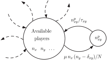
Figure 1: An illustration of the processes in the social dynamics. Players with strategies $x$ and $y$ meet and engage in contests. When a contest ends, the participants return to the available state. The number of individuals of strategy $x$ in the available state is $n_{x}$, and the number of ongoing contests between players with these strategies is given by $n^{\text{p}}_{xy}$, for a given pair of strategies $(x,y)$. The rates at which contests start and end are given along the arrows, where $\tau_{xy}$ is the expected duration of a $(x,y)$-game, and $N$ is the whole population size. The dotted arrows connect to the nodes for other pairs.

A contest between two individuals, with waiting-times $x$ and $y$, takes the form of the war of attrition game. In general, $x$ and $y$ may be stochastic variables, reflecting mixed strategies. From Section 4 and onward, we focus on pure strategies. The duration of the game is given by the smallest of the waiting-times. The player with the largest waiting-time gets the score 1, and the other player gets the consolation prize, i.e., the score $k$, with $0<k<1$. If both players have the same waiting-time, they both get an expected score of $(1+k)/2$.

At each instant a fraction $p_{\text{a}}$ of the population is available for playing, while the rest of the individuals are engaged in pair-wise contests. The total number of players with strategy $x$ in the population is denoted by $n^{\text{tot}}_{x}$, the number of available players with waiting-time $x$ is given by $n_{x}$, and the number of ongoing games between the players with waiting-times $x$ and $y$ is $n^{\text{p}}_{xy}$. It is convenient to treat the pairs $(x,y)$ and $(y,x)$ separately; though they are equivalent, it simplifies the calculations.

We assume that the time intervals between games are independent. Available players form ordered pairs $(x,y)$ for playing according to a Poisson process with rate $\mu(p_{\text{a}})\,n_{x}\,(n_{y}-\delta_{xy})/N$, where $\delta_{xy}$ equals one if $x=y$ and zero otherwise. Note that time is measured in units of $N$ for convenience: the number of events per unit of time remain finite for large $N$. The rate $\mu(p_{\text{a}})$ is a positive function of the fraction of available players, and may be used to model how the social dynamics depends on the availability of players. For a player, the expected time between the end of one contest and the onset of the next is $[2\,p_{\text{a}}\,\mu(p_{\text{a}})]^{-1}$. We illustrate the choice of $\mu(p_{\text{a}})$ by two examples. First, a model where players perform random walks, and occasionally meet and play. This corresponds to constant $\mu(p_{\text{a}})$. Second, a model where the expected time between games for a player is independent of the number of available players, corresponds to taking $\mu(p_{\text{a}})\propto p_{\text{a}}^{-1}$. In general, we assume that $\mu(p_{\text{a}})$ is chosen so that the expected time between games for a player is decreasing with $p_{\text{a}}$ or constant, and is bounded for $0\leq p_{\text{a}}\leq 1$.

When the population is finite, the social dynamics forms a Markov process and we know that there is a unique stationary distribution characterising the distribution of strategies in the different states.

In general, we should expect that players who are prepared to wait for a longer time (before finishing a game) enter the available state less frequently, and it is this effect that will result in an implicit time cost. We can find the equilibrium distribution, i.e., the expectation value of the number of individuals and pairs, by using the requirement that the expected number of pairs formed equals the number of pairs that finish playing, per unit of time:

$$\frac{\langle n^{\text{p}}_{xy}\rangle}{\tau_{xy}}=\frac{\mu(p_{\text{a}})}{N}\langle n_{x}\rangle\left(\langle n_{y}\rangle-\delta_{xy}\right),$$ (1)

where $\tau_{xy}$ is the expected duration of a game between a pair of players with strategies $x$ and $y$, respectively. By counting players with strategy $x$ that are available or playing, we get the relation

$$n^{\text{tot}}_{x}\ =\ \langle n_{x}\rangle+2\sum_{y}\langle n^{\text{p}}_{xy}\rangle\ =\ \langle n_{x}\rangle+2\,\frac{\mu(p_{\text{a}})}{N}\sum_{y}\tau_{xy}\langle n_{x}\rangle\left(\langle n_{y}\rangle-\delta_{xy}\right),$$ (2)

which can be used to solve for the equilibrium distribution for players in the available state, given a certain overall distribution of strategies.

We now focus on large populations. In the limit of large $N$, we take $u(x)$ to be the distribution of the waiting-time $x$ in the population ($u(x)\sim n^{\text{tot}}_{x}/N$), and $\rho(x)$ to be the distribution of $x$ among the available players ($\rho(x)\sim n_{x}/\sum_{y}n_{y}$). In the limit of many players it is convenient to consider a general distribution of waiting-times. Thus, (2) becomes

$$u(x)=p_{\text{a}}\,\rho(x)+2\,p_{\text{a}}^{2}\mu(p_{\text{a}})\int_{0}^{\infty}\tau(x,y)\,\rho(x)\,\rho(y)\,dy,$$ (3)

where $\tau(x,y)$ is the expected duration of a game between players with strategies $x$ and $y$. Note that different strategy spaces may be modelled by the appropriate function $\tau(x,y)$ of $x$ and $y$, where now $x$ (and $y$) is a parameter characterising the strategy rather than the explicit waiting-time. For instance, the set of mixed strategies with exponentially distributed waiting-times may be characterised by the expected waiting-time.

Since the expected time between contests for a player is $[2\,p_{\text{a}}\,\mu(p_{\text{a}})]^{-1}$, the expected number of games per unit of time is

$$N_{\text{G}}(x)=\left[\,\frac{1}{2\,p_{\text{a}}\,\mu(p_{\text{a}})}+\int_{0}^{\infty}\tau(x,y)\,\rho(y)\,dy\,\right]^{-1}.$$ (4)

We may now express $u(x)$ as

$$u(x)=2\,p_{\text{a}}^{2}\,\mu(p_{\text{a}})\,\rho(x)/N_{\text{G}}(x).$$ (5)

As an alternative, we may derive (5) from the ergodicity of the system. The fraction of the population with parameter $x$ that is in the available state is $p_{\text{a}}\,\rho(x)/u(x)$. A player with parameter $x$ spend a fraction $N_{\text{G}}(x)/[2\,p_{\text{a}}\,\mu(p_{\text{a}})]$ of the time in the available state. Since the onsets of two consecutive contests are assumed to be uncorrelated, the two fractions must be equal, and we again arrive at (5).

3 Evolutionary dynamics

It is assumed that the population evolves so that players with strategies that get higher scores per unit time increase their fraction of the population, leading to a change in the distribution $u(x,t)$ at time $t$. Further, it is assumed that the evolutionary dynamics and the social dynamics occur on separate time scales so that the equilibrium distribution given by (3) can be used to determine the scores of the different players. Then, on the evolutionary time scale, the population dynamics is given by the replicator dynamics,

$$\frac{\partial u(x,t)}{\partial t}=u(x,t)\left[\,f(x,t)-{\bar{f}(t)}\,\right],$$ (6)

where $f(x,t)$ is the expected fitness of a player with strategy $x$, per unit of time in the social dynamics, and $\bar{f}(t)$ is the average fitness in the whole population at time $t$,

$$\bar{f}(t)=\int_{0}^{\infty}u(x,t)\,f(x,t)\,dx.$$

To simplify the notation, let us suppress the explicit time dependence in the notation and write $u(x)$ for $u(x,t)$ etc. The expected fitness of a player with strategy $x$ is the product of two factors, the expected score per game and the number of games per unit of time:

$$f(x)=N_{\text{G}}(x)\int_{0}^{\infty}\left[\,k+(1-k)\,P(x,y)\,\right]\,\rho(y)\,dy,$$ (7)

where $P(x,y)$ is the probability that a player with strategy $x$ is the winner in a game against a player with strategy $y$.

A player can increase the expected score per game by waiting longer, but that will decrease the number of games played per unit of time, and we get an implicit cost due to the longer engagement in the games. Therefore, whether it is advantageous for a player to increase or decrease the waiting-time depends on the distribution of strategies in the population.

Note that the sum of the scores in each game is $1+k$, and the total number of games per unit of time is $2p_{\text{a}}^{2}\mu(p_{\text{a}})$. From this we see a general connection between average fitness and the fraction of available players:

Lemma 1

When the population is in equilibrium with respect to the social dynamics, the average fitness in the population is

$$\bar{f}=p_{\text{a}}^{2}\,\mu(p_{\text{a}})\,(1+k),$$ (8)

for any set of strategies.

4 Deterministic strategies

The formalism presented in the previous sections applies to both pure and mixed strategies. In the following, we assume pure strategies, so that each player is prepared to wait a given time $x$, and the population is then characterised by a distribution $u(x)$ over the waiting-times. When a player $A$ with strategy $x$ meets a player $B$ with strategy $y$, the probability of winning for player $A$ is $P(x,y)=\theta(x-y)$, where $\theta(z)$ is one if $z>0$, $1/2$ if $z=0$ and zero otherwise. The duration of the game is given by $\tau(x,y)=\min(x,y)$.

When there is an atom at infinity (i.e., a finite share of the population with infinite waiting-time), the players that wait indefinitely always get a fitness of zero, since the expected score per game is bounded from above by one, and the expected time per game is infinite (c.f. (7)). Thus, this strategy is dominated by all other strategies, and in the following we assume there is no atom at infinity.

In Fig. 2, we show the time evolution of the distribution of waiting-times in the population, in the case of constant $\mu(p_{\text{a}})$, for consolation price $k=0.1$ and $k=0.3$, from numerical integration of the replicator dynamics (c.f. (6)). The initial distribution is taken to be proportional to the inverse waiting-time over the interval shown in the figure, and zero elsewhere. For $k=0.1$, we find that the dynamics seems to converge to a limit cycle, and for $k=0.3$ it seems to converge to a stationary distribution.

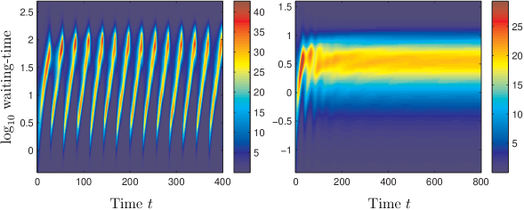
Figure 2: The time evolution of the distribution of waiting-times in the population, in the case of constant $\mu(p_{\text{a}})$, for consolation price $k=0.1$ (left) and $k=0.3$ (right). For clarity, we show the distribution of the base-10 logarithm of the waiting-time in the population. The colour-bars show the value corresponding to each colour in the figures. For $k=0.1$, the dynamics seems to converge to a stable limit cycle, and for $k=0.3$ it seems to converge to a stationary distribution.

5 Stationary distributions

The numerical simulations show that the systems seems to converge to a stationary distribution for some values of the consolation prize $k$. In this section, we derive the form of this distribution.

A stationary distribution $u(x)$ is determined by the requirement $f(x)=\bar{f}$ wherever $u(x)>0$. With the cumulative distribution of the available players, $\Phi(x)=\int_{0}^{x}\!\rho(y)\,dy$, we can use (4) and (7) to express the stationarity condition as

$$\Phi(x)+k\big{(}1-\Phi(x)\big{)}=\bar{f}\,\left[\frac{1}{2\,p_{\text{a}}\,\mu(p_{\text{a}})}+\int_{0}^{x}y\,\rho(y)\,dy+x\big{(}1-\Phi(x)\big{)}\right].$$ (9)

Next, we take the derivative of this equation with respect to $x$:

$$(1-k)\,\rho(x)=\bar{f}\,[\,x\,\rho(x)-x\,\rho(x)+1-\Phi(x)\,]=\bar{f}\,[\,1-\Phi(x)\,].$$

Since $\Phi(0)=0$ and $\Phi(\infty)=1$, we see that there is a unique solution

$$\Phi(x)=1-e^{-\lambda x}\text{ where }\lambda=\frac{\bar{f}}{1-k}=p_{\text{a}}^{2}\,\mu(p_{\text{a}})\,\frac{1+k}{1-k}$$ (10)

by Lemma 1. By inserting the solution (10) into (9) we find the fraction of available players in the population:

$$p_{\text{a}}=\frac{2\,k}{1+k}.$$

Given the distribution of strategies among the available players, the distribution $u(x)$ of strategies in the population can be calculated from (3). The results are summarised in the following theorem:

Theorem 2

In a population of players with deterministic waiting-times, there is a unique stationary distribution $u(x)$ involving all strategies $x$, given by

$$u(x)=\frac{2\,\lambda}{1+k}\left[\,e^{-\lambda\,x}-(1-k)\,e^{-2\,\lambda\,x}\,\right]\text{, where }\lambda\ =\ \frac{4\,k^{2}}{1-k^{2}}\,\mu(\frac{2\,k}{1+k}).$$ (11)

The fraction of available players is then $p_{\text{a}}=2\,k/(1+k)$ and the expected fitness of all players is

$$\bar{f}=\frac{4\,k^{2}}{1+k}\,\mu\big{(}\frac{2\,k}{1+k}\big{)}.$$

Furthermore, the distribution of strategies among the available players is exponentially distributed:

$$\rho(x)=\lambda\,e^{-\lambda\,x}.$$

From Theorem 2, we obtain the distribution of strategies amongst the players engaged in games at the stationary distribution as

$$\frac{u(x)-p_{\text{a}}\,\rho(x)}{1-p_{\text{a}}}=2\lambda e^{-\lambda x}-2\lambda e^{-2\lambda x}.$$

The stationary distribution is shown in Fig. 3 for three values of the consolation prize $k$. The strategies of the available players are exponentially distributed, as is the stationary distribution in the original war of attrition (Maynard Smith, 1974). In our model, however, the stationary distribution is decreasing for short waiting-times. This is due to that strategies with short waiting-time are over-represented among the available players, compared to the distribution of strategies in the population. Of the players with waiting-time $x$, a fraction $p_{\text{a}}\,\rho(x)/u(x)=k/[1-(1-k)\exp(-\lambda x)]$ is in the available state, at the stationary distribution. This means that, despite the risk for getting stuck in long games, players with long waiting-times will spend at least a fraction $k$ of their time in the available state.

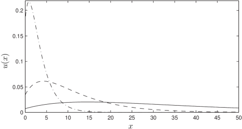
Figure 3: The stationary distribution $u(x)$ for the consolation prize $k=0.1$ (solid line), $k=0.17$ (dashed line) and $k=0.3$ (dashed and dotted line).

6 Stability of the stationary distribution

Although there exist stationary distributions for all $k\in(0,1)$ as seen in Fig. 3, we note from Fig. 2 that there could be a fundamental difference in the dynamics for different consolation prizes $k$. In order to better understand the dynamics of the model, we investigate the stability of the stationary distribution (11), as function of the consolation prize $k$. We give analytical results for infinitesimal perturbations of the stationary distribution, as well as results from numerical simulations, in order to explore the global convergence to the stationary distribution.

Both the stationary distribution $u(x)$ and the distribution of strategies among available players, $\rho(x)$, are polynomials in $e^{-\lambda\,x}$. In order to simplify the analysis of the stability of the stationary distribution, and also to facilitate more accurate simulations, we map the strategy $x$ to a point $s$ in the unit interval through

$$s=e^{-\lambda x}\quad\text{with}\quad\lambda=\frac{4\,k^{2}}{1-k^{2}}\,\mu\big{(}\frac{2\,k}{1+k}\big{)}.$$

Thus the whole range of waiting-times $[0,\infty)$ is represented by the interval $(0,1]$. The distribution of $s$ in the population is then $u_{s}(s)=u(-\lambda^{-1}\,\ln s)/(\lambda s)$. Similarly, we define $f_{s}(s)$ as the fitness of a player with parameter $s$.

In order to be specific, in the following we restrict the analysis of the stability properties to the case where $\mu(p_{\text{a}})$ is constant. It is straight-forward to extend the analysis to other $\mu(p_{\text{a}})$. With the functions

$$g(s) = \frac{1+k}{2\,k}\,\frac{1}{\lambda\,s}\,p_{\text{a}}\,\rho(-\frac{\ln s}{\lambda})\quad\text{and}$$

$$h(s) = k+(1-k)\,\lambda\int_{0}^{1}\tau(\,-\frac{\ln s}{\lambda},-\frac{\ln t}{\lambda})\,g(t)\,dt,$$

we can express (5) as

$$u_{s}(s)=2\,g(s)\,h(s)/(1+k).$$ (12)

Note that $g(s)$ is proportional to the distribution of $s$ among the available players. For convenience, we now measure time in units of $\bar{f}$ in the stationary distribution, $4k^{2}/(1+k)$. In the new units, we have $f_{s}(s)=m(s)/h(s)$ and $\bar{f}=\hat{g}^{2}$, where

$$m(s)=\int_{0}^{1}S(-\frac{\ln s}{\lambda},-\frac{\ln t}{\lambda})\,g(t)\,dt\quad\text{and}\quad\hat{g}=\int_{0}^{1}g(t)\,dt.$$

The time evolution of the distribution of $s$, (6), is then

$$\frac{\partial u_{s}(s)}{\partial t}=\frac{2}{1+k}\,g(s)\,[\,m(s)-\hat{g}^{2}\,h(s)\,].$$

For deterministic strategies, we have

$$\tau(-\frac{\ln s}{\lambda},-\frac{\ln t}{\lambda}) = -\frac{1}{\lambda}\max(\,\ln s,\ln t\,)$$

$$S(-\frac{\ln s}{\lambda},-\frac{\ln t}{\lambda}) = \theta(t-s)+k\,\theta(s-t),$$

so at the stationary distribution (11) we get $g(s)=\hat{g}=1$ and $\ h(s)=m(s)=1-(1-k)s$. Thus, in the parameter $s$ the stationary distribution becomes

$$u_{s}(s)=2\,\left[1-(1-k)s\right]/(1+k).$$ (13)

6.1 Evolutionary stability

There are many different ways of characterising the stability of a distribution under the evolutionary dynamics in the literature (see e.g. Hines (1987) for a review). One of the most commonly used definitions of stability is to test whether the stationary distribution can resist an invasion from a population with distribution $q_{s}(s)$ at a level $\eta$, for all positive values of $\eta$ in a neighbourhood of zero. The distribution of strategies in the population after the invasion is thus $(1-\eta)\,u_{s}(s)+\eta\,q_{s}(s)$. Then $u_{s}(s)$ is an evolutionarily stable distribution if and if only the expected fitness among the players in the old distribution is higher than the fitness among the invaders:

$$\int_{0}^{1}u_{s}(s)\,\tilde{f}_{s}(s)\,ds>\int_{0}^{1}q_{s}(s)\,\tilde{f}_{s}(s)\,ds,$$

where $\tilde{f}_{s}(s)$ is the fitness of a player with strategy $s$ in the population with distribution $\tilde{u}_{s}(s)$. Now expand $\tilde{f}_{s}(s)$ for small $\eta$: $\tilde{f}_{s}(s)=f_{s}(s)+\delta f_{s}(s)\,\eta+O(\eta^{2})$, where $\delta f_{s}(s)=\mathcal{F}[\,\delta u_{s}(s)\,]$ is a functional of the perturbation $\delta u_{s}(s)=\tilde{u}_{s}(s)-u_{s}(s)$. Since $f_{s}(s)=\bar{f}$ at the stationary distribution,

$$\int_{0}^{1}[\,u_{s}(s)-q_{s}(s)\,]\,f_{s}(s)\,ds=\int_{0}^{1}[\,u_{s}(s)-q_{s}(s)\,]\,\bar{f}\,ds\ =\ 0,$$

so $u_{s}(s)$ is evolutionarily stable if and only if for all small enough perturbations $\delta u_{s}(s)$,

$$\int_{0}^{1}\delta u_{s}(s)\,\mathcal{F}[\,\delta u_{s}(s)\,]\,ds<0.$$

Since we know how to calculate the distribution $u_{s}(s)$ from the distribution of available players, it is convenient to express a perturbation $\delta u_{s}(s)$ as a perturbation in the availability of the strategies using (12):

$$\delta u_{s}(s)=\frac{2}{1+k}\mathcal{L}[\,\delta g(s)\,]\text{ where }\mathcal{L}[\,\delta g(s)\,]=\delta[\,g(s)h(s)\,].$$

At the stationary distribution, we get

$$\mathcal{L}[\,\delta g(s)\,]=[\,1-(1-k)s\,]\,\delta g(s)-(1-k)\,\int_{0}^{1}\max(\ln s,\ln t)\,\delta g(t)\,dt.$$

Since $\delta u_{s}(s)$ is normalised to zero, we have that the corresponding perturbation $\delta g(s)$ must obey

$$0=\int_{0}^{1}\mathcal{L}[\delta g(s)]\,ds=\int_{0}^{1}[\,2-k-2\,(1-k)\,s\,]\,\delta g(s)\,ds.$$ (14)

With $\delta f_{s}(s)=\mathcal{B}[\,\delta g(s)\,]$, we find

$$\mathcal{B}[\,\delta g(s)\,]=\delta[\,\frac{m(s)}{h(s)}\,]=\frac{\delta m(s)\,h(s)-m(s)\,\delta h(s)}{h(s)^{2}}=\frac{\delta m(s)-\delta h(s)}{1-(1-k)\,s}$$

at the stationary distribution (13), where

$$\delta m(s)-\delta h(s)=\int_{0}^{s}ds\,[\,k+(1-k)\,\ln\,s\,]\,\delta g(t)+\int_{s}^{1}ds\,[\,1+(1-k)\,\ln\,t\,]\,\delta g(t).$$

Thus $u_{s}(s)$ is not evolutionarily stable if we can find a perturbation $\delta g(s)$ such that

$$\mathcal{M}[\,\delta g(s)\,]=\int_{0}^{1}\mathcal{L}[\,\delta g(s)\,]\mathcal{B}[\,\delta g(s)\,]\,ds>0.$$

We expand the perturbation $\delta g(s)$ in the shifted Legendre polynomials $\bar{P}_{i}(s)$ (Abramowitz and Stegun, 1972), and maximise $\mathcal{M}[\,\delta g(s)\,]$ subject to the normalisation condition (14) and $\int_{0}^{1}\mathcal{L}[\,\delta g(s)\,]^{2}\,ds=1$. In order to find a numerical solution, we restrict the analysis to the $n+1$ first Legendre polynomials: $\delta g(s)=\sum_{i=0}^{n}g_{i}\,\bar{P}_{i}(s)$. Ignoring the higher order polynomials amounts to ignoring highly oscillatory contributions to the perturbation $\delta g(s)$.

With $n=50$ we find that for $k<k^{*}_{\text{ess}}\approx 0.5196$ there is a positive maximum of $\mathcal{M}[\,\delta g(s)\,]$, but when $k>k^{*}_{\text{ess}}$ all extreme values are negative. Thus we have evidence that there is no evolutionarily stable strategy for $k<k^{*}_{\text{ess}}$. For $k>k^{*}_{\text{ess}}$ we have not shown that the distribution is evolutionarily stable, but that it is likely so. The value $k^{*}_{\text{ess}}$ seems not to be sensitive to the number of Legendre polynomials $n$ used in the expansion of $\delta g(s)$, when $n\gtrsim 30$.

We have also performed these calculations for the case $\mu(p_{\text{a}})\propto p_{\text{a}}^{-1}$. For $n=50$ we find $k^{*}_{\text{ess}}\approx 0.6738$, and again the value of $k^{*}_{\text{ess}}$ seems to converge when $n$ is large enough (i.e. $n\gtrsim 30$).

Note that, in Fig. 2, the distribution seems to converge to the stationary distribution for $k$ as low as $0.3$. This indicates that evolutionary stability of the stationary distribution implies dynamical stability, but that the converse does not hold. In the following section, we address this issue.

6.2 Dynamical stability

We examine the long-term response of the replicator dynamics to a small perturbation $\delta u_{s}(s)$ in the composition of the population, around the stationary solution:

$$\frac{\partial\delta u_{s}(s)}{\partial t}=\frac{2}{1+k}\,\delta[\,g(s)\,m(s)-\hat{g}^{2}\,g(s)\,h(s)\,].$$ (15)

With the linear operator $\mathcal{A}[\delta g(s)]=\delta[\,g(s)\,m(s)-\hat{g}^{2}\,g(s)\,h(s)\,]$, we may write (15) in terms of the time evolution of the corresponding perturbation $\delta g(s)$ as:

$$\frac{\partial}{\partial t}\mathcal{L}[\delta g(s)]=\mathcal{A}[\delta g(s)].$$ (16)

Note that the perturbation $\delta g(s)$ is subject to the constraint (14). See Appendix A for the details of $\mathcal{A}$. In order to find whether a perturbation $\delta g(s)$ grows or decays, we look for solutions to (16) on the form $\delta g(s)=\phi(s)\,e^{\gamma t}$, where $t$ is the evolutionary time. The perturbation $\delta g(s)$ grows if and only if $\gamma$ has a positive real part. Thus, we find that $\gamma$ and $\phi(s)$ must be solutions to the generalised eigenvalue problem

$$\gamma\,\mathcal{L}[\phi(s)]=\mathcal{A}[\phi(s)].$$ (17)

Note that this is equivalent to solving the eigenvalue equation $\frac{\partial}{\partial t}\delta u_{s}(s)=\gamma\,\delta u_{s}(s)$.

In order to find good (numerical) approximations for the eigenvalues and eigenvectors, we again expand the linear operators $\mathcal{L}$ and $\mathcal{A}$ in the $n+1$ first shifted Legendre polynomials, so the eigenvector $\phi(s)$ is determined by the coefficients $a_{i}$ in the expansion $\phi(s)=\sum_{i=0}^{n}a_{i}\,\bar{P}_{i}(s)$. See Appendix A for details of how to solve for the coefficients $a_{i}$ numerically.

The perturbation corresponding to an eigenvector $\phi(s)$ grows at a rate given by the real part of the corresponding eigenvalue, $\textrm{Re }\gamma$. The growth rate for the different eigenvectors are shown in Fig. 4, as a function of the consolation prize $k$. For $k^{*}_{\text{dyn}}<k<1$, where $k^{*}_{\text{dyn}}\approx 0.1675$, there is no eigenvalue with positive real part. The value of $k^{*}_{\text{dyn}}$ does not seem to be sensitive to the number of Legendre polynomials in the expansion, when $n$ is large enough ($n\gtrsim 20$). Thus, in this region all sufficiently small perturbations will decay asymptotically, and the stationary distribution $u_{s}(s)$ is dynamically stable. As a consequence of this, the population will resist invasion of any mixed strategy, except the strategy $p(x)=\lambda\,e^{-\lambda\,x}$, where $x$ is the waiting-time and $\lambda$ is given by Theorem 2. This strategy mimics a randomly chosen available player in the stationary distribution, so all players get the same fitness values as before. We also show an estimate of the growth rate from simulations (see the circles in Fig. 4), and find good agreement with the growth rate predicted by the leading eigenvalue, in the region where the growth rate is positive.

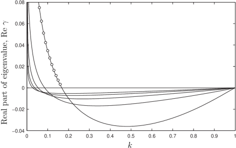
Figure 4: The real part of the 11 largest eigenvalues (ordered by modulus) as a function of the consolation prize $k$, from the expansion in the 51 first Legendre polynomials. We also show the growth rate for a small perturbation, estimated from simulations (white circles) for some values of $k$.

In general, a perturbation does not only grow or decay but also oscillates with characteristic frequencies. In Fig. 5 we show the period of these oscillations, given by $2\pi/|\textrm{Im }\gamma|$, as a function of $k$. The black points indicate where the real part of the eigenvalue becomes positive (see Fig. 4). Estimated values from simulations are shown as white circles, and we find good agreement with the period rate predicted by the leading eigenvalue.

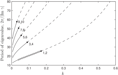
Figure 5: The period $2\pi/|\textrm{Im }\gamma|$ as a function of the consolation prize $k$, where $\textrm{Im }\gamma$ is the imaginary part of the eigenvalue $\gamma$. For each eigenvalue, the curve is drawn solid where the real part is positive, and is drawn dashed where it is negative. The black dots shows the points of transition from negative to positive real parts, and the number by the dots is the number of the eigenvalue when sorted by decreasing magnitude. We also show the period of a small perturbation, estimated from simulations (white circles) for some values of $k$.

When $\mu(p_{\text{a}})\propto p_{\text{a}}^{-1}$, the calculations of the dynamical stability gives $k^{*}_{\text{dyn}}\approx 0.1197$, when $n=50$. We find as before, that this limit converges quickly for $n$ large enough (i.e. $n\gtrsim 20$).

7 Long-term evolution as a function of the initial distribution

In order to assess the global convergence of the dynamics to the stationary distribution (c.f. Fig. 2), we have compared the asymptotic evolution of $u_{s}(s)$ when started from different initial distributions: $u_{s}(s)=1$, $u_{s}(s)=2(1-s)$, $u_{s}(s)=2(1+s)/3$, $u_{s}(s)=2s$, and $u_{s}(s)=6s(1-s)$. In the simulations, the continuous parameter space $[0,1]$ was approximated by $1,000$ equally spaced atoms in the interval $(0,1)$, and time was divided into discrete steps of $0.1$ units of time. The first $20,000$ units of time was considered transient, and was discarded. The deviation from the stationary distribution $u^{*}_{s}(s)=2\left[1-(1-k)s\right]/(1+k)$ was then measured at $100$ times, $10$ units of time apart, by the Kullback distance (Kullback, 1959)

$$K[u_{s}(s);u^{*}_{s}(s)]=\int_{0}^{1}u^{*}_{s}(s)\ln\frac{u^{*}_{s}(s)}{u_{s}(s)}\,ds.$$

The Kullback distance is always non-negative, and since $u^{*}_{s}(s)\geq 0$ for all $s$, it is zero if and only if $u_{s}(s)=u^{*}_{s}(s)$ for all $s$ (Kullback, 1959). Second, the Kullback distance is invariant under a change of variables, so it does not matter which parameter (e.g. $x$ or $s$) we use to characterise a strategy. From the samples we estimate the time average and standard deviation of the distance. In Fig. 6 we show the asymptotic average Kullback distance, plus and minus one standard deviation, as a function of $k$ for the different initial distributions above.

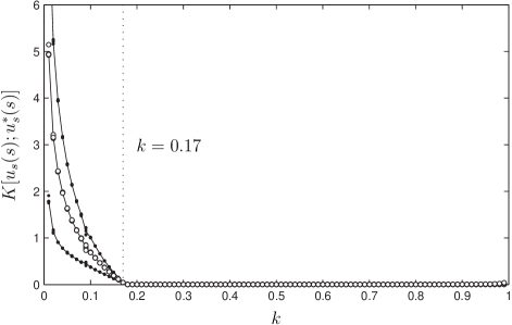
Figure 6: The asymptotic time-averaged Kullback distance $K[u_{s}(s);u^{*}_{s}(s)]$ from the stationary distribution $u^{*}_{s}(s)$ (see (13)) to the distribution $u_{s}(s)$, from five different initial distributions (white circles). The points corresponding to one standard deviation up and down is shown as black dots, with one dot for each initial distribution. Solid lines are averages over all initial distributions. The dotted vertical line show $k=0.17$, denoting the point where the stationary distribution becomes stable. Convergence to the stationary distribution is slow for $k$ close to one, since the fitness differences are small. Note that the results are almost indistinguishable for the five different initial distributions.

We summarise the results from these experiments as follows: First, for $k>0.17$ we find that the distribution of waiting-times converges to the stationary distribution for the initial distributions above. Second, for $k<0.17$ we find that the average of the asymptotic distance, and also its standard deviation, is almost identical for the initial distributions above. Inspection of the time evolution of the distribution gives that the dynamics seems to converge to a limit cycle (c.f. Fig. 2 for an example). This indicates that the dynamics converge to stable limit cycle for these values of $k$. Third, since the initial distributions was chosen to be very different (some dominated by large waiting-times, some by low waiting-times and other intermediate) we conjecture that these results hold for any initial distribution with full support.

8 Explicit time cost

We return to models of an explicit cost for the duration of a contest. Let $S(x)$ be the expected score per game for a player with waiting-time $x$ (the cost not included), and let $D(x)$ be expected duration of a contest. Suppose the cost per unit of time during the contest is $c$. The expected fitness is then given by

$$f(x)=N_{\text{G}}(x)\left[S(x)-c\,D(x)\right].$$

Since by (4), $N_{\text{G}}(x)=[\,1/\nu+D(x)\,]^{-1}$ where $\nu=2\,p_{\text{a}}\,\mu(p_{\text{a}})$, we have

$$f(x)=N_{\text{G}}(x)\,S(x)-c+c\,N_{\text{G}}(x)/\nu.$$

Note that since $N_{\text{G}}(x)$ is decreasing with the waiting-time, players with small waiting-time are less influenced by a high cost $c$, compared to players with higher waiting-time.

The average fitness in the population is by (5) and (8):

$$\bar{f} = \int_{0}^{\infty}\frac{p_{\text{a}}\,\nu\,\rho(x)}{N_{\text{G}}(x)}\left[N_{\text{G}}(x)\,S(x)-c+c\,N_{\text{G}}(x)/\nu\right]\,dx$$

$$= p_{\text{a}}\,\nu\,\frac{1+k}{2}-c+c\,p_{\text{a}}=(1+k)\,p_{\text{a}}^{2}\,\mu(p_{\text{a}})-c\,(1-p_{\text{a}}).$$

Thus, the average fitness is lowered by a factor $c\,(1-p_{\text{a}})$ by the introduction of the cost $c$.

We derive the stationary distribution with positive cost $c$ from

$$S(x)-c\,D(x)=\bar{f}\,[\,1/\nu+D(x)\,]$$

by letting $f(x)=\bar{f}$ as in Section 5. We find that for any cost $c>0$, there is a unique stationary distribution $u(x)$ involving all strategies $x$, given by

$$u(x)=(2-p_{\text{a}})\,\lambda\,e^{-\lambda\,x}-(1-p_{\text{a}})\,2\lambda\,e^{-2\lambda\,x}$$

where $\lambda=p_{\text{a}}^{2}\,\mu(p_{\text{a}})/(1-p_{\text{a}})$. The fraction of available players $p_{\text{a}}$ is the solution to

$$2\,k\,p_{\text{a}}\,\mu(p_{\text{a}})-(1+k)\,p_{\text{a}}^{2}\,\mu(p_{\text{a}})+c\,(1-p_{\text{a}})=0.$$ (18)

The distribution of strategies among the available players is $\rho(x)=\lambda\,e^{-\lambda\,x}$.

Note that since $\mu(p_{\text{a}})$ is assumed to be bounded, $p_{\text{a}}\rightarrow 1$ as $c\rightarrow\infty$ in order to fulfill (18). In the limit of $c=0$ we recover $p_{\text{a}}=2k/(1+k)$, and for $c>0$ we have $p_{\text{a}}>2k/(1+k)$. We now give the solution to (18) for two cases of special interest: for constant $\mu(p_{\text{a}})$ and for $\mu(p_{\text{a}})\propto p_{\text{a}}^{-1}$, we have

$$p_{\text{a}}=\frac{2\,k-c+\sqrt{(2\,k-c)^{2}+4\,(1+k)\,c}}{2\,(1+k)}\text{ and }p_{\text{a}}=\frac{2\,k+c}{1+k+c}\text{, respectively.}$$

We will now show that one can find a $\tilde{k}$, such that the fitness of the strategy with explicit time cost $c$ and the consolation prize $k$, equals the fitness of the strategy with no explicit cost and the consolation prize $\tilde{k}$.

With the probability of winning a game, $P(x)=\int_{0}^{x}\rho(y)\,dy$, we have the expected score $S(x)=k+(1-k)\,P(x)$, and thus the fitness $f(x)$ may be written

$$f(x)=\left(\frac{c}{\nu}+k\right)\!N_{\text{G}}(x)+(1-k)\,N_{\text{G}}(x)\,P(x)-c.$$

We compare this expression to the fitness of the strategy when $k=\tilde{k}$ and $c=0$:

$$f_{c\,=\,0}(x)=\tilde{k}\,N_{\text{G}}(x)+(1-\tilde{k})\,N_{\text{G}}(x)\,P(x).$$

Since the growth rate of a strategy is proportional to the difference between the fitness of the strategy and the average fitness in the population, it does not matter if we add a number to all fitness values and multiply them with a positive number. Note that these numbers may change with time, as long as they are the same for all strategies. Thus, we see that if we set

$$f_{c\,=\,0}(x)/(1-\tilde{k})=(f(x)+c)/(1-k)$$

we get equality for all $x$ if and only if

$$\frac{\tilde{k}}{1-\tilde{k}}=\frac{c/\nu+k}{1-k}\quad\Leftrightarrow\quad\tilde{k}=1-\frac{1-k}{1+c/\nu}.$$ (19)

Note that $c/(c+\nu)\leq\tilde{k}\leq 1$ for all $k$, and especially $\tilde{k}>k$ when $c>0$.

When the expected time between games, $\nu$, is independent of the fraction of available players in the population, $\mu(p_{\text{a}})\propto p_{\text{a}}^{-1}$, then $c/\nu$ is constant in time. It follows that the dynamical equations are exactly the same for both sets of parameters, apart from a scaling of the evolutionary time.

When $\nu$ depends on $p_{\text{a}}$, we cannot map the dynamics for a given combination of $k$ and $c$ onto $k=\tilde{k}$ and $c=0$, since the equivalent consolation price $\tilde{k}$ would then change with time (unless the population is stationary). However, since $\tilde{k}$ increases with decreasing $\nu$ according to (19), we expect that the domain of stability is increased significantly.

9 Comparison to other models

In this section, we discuss how our results pertain to the models of Cannings and Whittaker (1994) and Hines (1977).

9.1 The model of Hines

In Hines’ model animals forage for food, and the events of finding food are assumed to be a Poisson process with rate $\alpha$ per animal. Each food parcel corresponds to one fitness unit. Sometimes the animal gets to consume the food parcel without challenge, but with probability $\pi$ the animal is challenged and enters a war of attrition for the food parcel. The time spent foraging and in contests are assumed to be statistically independent. During foraging, the animal has energy consumption $\mu_{\text{F}}$ fitness units per unit of time, and during a contest the corresponding energy consumption is $\mu_{\text{C}}$ fitness units per unit of time.

Since the evolutionary dynamics modelled by replicator dynamics is invariant when the fitness undergo addition of constants and multiplication by positive constants, we find a relation between the the consolation prize $k$ used in our model, in the absence of explicit time cost, and the parameters in Hines’ model:

$$k=\frac{\alpha(1-\pi)+\mu_{\text{C}}-\mu_{\text{F}}}{\alpha+\mu_{\text{C}}-\mu_{\text{F}}}.$$ (20)

Note that the right hand side is positive for realistic choices of the parameters. Naturally, $\pi=0$ corresponds to $k=1$, since any food parcel found is uncontested. With $\mu_{\text{C}}=\mu_{\text{F}}$, the relation is simply $k=1-\pi$.

The relation (20) completely maps the model by Hines onto our model. Thus, the whole range of behaviours of Hines’ model is captured by the single value of $k$. Specifically, we note that the stationary distribution characterising our model and the corresponding stability analysis in Section 6 apply.

9.2 The model of Cannings and Whittaker

In (Cannings and Whittaker, 1995) the authors studied a model where players repeatedly meet each other in the war of attrition game, with a score of zero for the loser, i.e. $k=0$, and with an explicit time cost $c$. The waiting-times are restricted to the set of positive integers, and the players wait one unit of time between games. In their model, as in Hines’ and ours, it is assumed that players finishing faster get to play more frequently. In addition to this they also introduced discounting, where scores received earlier in a sequence of games are valued higher.

We apply our method as described in Section 2 to analyse the model. We find: Initial correlations between players decay as the evaluation period proceeds. Hence, in the limit of long evaluation periods, and when the discount rate is sufficiently low, the average fitness over the evaluation period, for a player, equals the expected fitness in the equilibrium distribution. The time between games $\nu=1$ gives $\mu(p_{\text{a}})=(2p_{\text{a}})^{-1}$. Since $\nu$ is constant, we can map the evolutionary dynamics onto the dynamics in the absence of explicit time cost and with consolation prize $k=c/(1+c)$. In Appendix B we derive the unique stationary distribution (involving all waiting-times), for this model. With $\rho_{i}$ as the fraction of the available players with waiting-time $i$, and with $u_{i}$ as the corresponding fraction of the population, we find

$$\rho_{1}=4\,a-\frac{2\,c}{1+2\,c},\qquad u_{1}=\frac{8\,a\left(2\,a-c\right)}{1+2\,c},$$

where $a=(3+6\,c-\sqrt{9+4\,c+4\,c^{2}})/8$. For $i\geq 2$, we find

$$\rho_{i} = \left(4\,a-1-2\,c\right)\!\left({\sqrt{1+a^{2}}}-1-a\right)\!{\left({\sqrt{1+a^{2}}}-a\right)}^{i-2}\quad\text{and}$$

$$u_{i} = \frac{2\,a\,\rho_{i}\left[a+2\,a\,c-(1+a)\rho_{i}-(\sqrt{1+a^{2}}-1)(5+2\,c+\rho_{i})\right]}{{\left(1+a-\sqrt{1+a^{2}}\right)}^{2}\left(1+2\,c\right)}.$$ (21)

Numerical simulations show that the dynamics converge to the stationary distribution when $c\gtrsim 0.13$. For smaller costs, the dynamics seems to converge to a stable limit cycle. Thus, the dynamical properties of this model are similar to the dynamical properties of our model where $\mu(p_{\text{a}})\propto p_{\text{a}}^{-1}$, and where the waiting-time may take any positive value.

10 Discussion and concluding remarks

We study the evolutionary dynamics of a population, where individuals interact according to a social dynamics. In particular we study a variation of the war of attrition (or the waiting-game) in which the explicit time cost is replaced by an implicit cost, due to less frequent game participation for those involved in longer contests. Players are characterised by the waiting-time, the time they are prepared to wait before they give up to the opponent. The player with the larger waiting-time gets the score $1$, while the other player gets the consolation price $k\in[0,1]$. Players are in one of two states: either they are engaged in a game or they are available for entering a new game. We analyse the time evolution of the distribution of strategies in the population when the population size is fixed, and players produce offspring that survive to the next generation in proportion to their fitness.

The fitness of a player is a product of two factors: the first is the expected score per game, determined by the probability of winning against a randomly chosen player, and the second is the number of games played per unit time. There are two ways a player may attempt to increase its fitness: it can either try to increase the probability of winning the games played (by increasing the waiting-time), or to increase the expected number of games (by decreasing the waiting-time). In general, it is not possible for a player to have both a high chance of winning a game, and to play many games per unit of time. Thus, the second factor reflects an implicit time cost.

We summarise our results as follows: First, the average fitness in the population is determined by the fraction of the population that is available, or equivalently, by the average duration of games.

Second, when players follow deterministic strategies there is, for all $k$, a unique stationary population involving all waiting-times. When the consolation prize $k$ approaches the score of 1 for winning a game, we find that the stationary distribution is characterised by strategies with small waiting-times. For small $k$, the stationary distribution is characterised by large waiting-times: as $k$ approaches zero, the average waiting-time in the stationary population diverges.

Third, the stability of the stationary state depends on the consolation prize $k$. The stationary state is evolutionarily stable for large enough values, $k\gtrsim 0.5196$ for constant $\mu$, and $k\gtrsim 0.6738$ for $\mu\propto p_{\text{a}}^{-1}$. Below this level the evolutionary stability is lost, but the system exhibits a weaker form of stability, dynamic stability, when $k\gtrsim 0.1675$ for constant $\mu$, and when $k\gtrsim 0.1197$ for $\mu\propto p_{\text{a}}^{-1}$. Here perturbations may lead to a transient oscillatory behaviour, after which the system is brought back to the stationary state again. Although the perturbations eventually vanish, the transient period may be very long. For small $k$ the stationary state is unstable, showing an oscillatory behaviour in the average waiting-time. It shall be noted that, in this model evolutionary stability does not imply dynamical stability.

Fourth, the numerical simulations indicate that the stationary distribution is a global attractor when $k$ is in the dynamically stable region. When the stationary state is not dynamically stable, the dynamics seems to converge to a stable limit cycle from any initial distribution. The period and shape of the limit cycle depends on $k$.

Fifth, there is an affine transformation of the fitness values in a population, from a population with positive time cost $c$ to a population with no explicit time cost, where the new consolation price $\tilde{k}$ is now a function of the explicit time cost, the original consolation price $k$, and the expected time between games in the original population. When the time between games is independent of the fraction of available players in the population, the time evolution of the two populations are thus the same.

Sixth, the implicit time cost is increasing with the explicit time cost $c$. Thus, players with small waiting-time have an advantage in that they are less affected by this cost.

Seventh, the models of Hines (1977) and Cannings and Whittaker (1994) both correspond to a time between games independent from the population composition, hence our methods and results apply to these models, when the number of games per generation is large.

The oscillatory behaviour of the dynamics for small $k$ can be intuitively understood by the following simplified arguments: if the consolation price $k$ is small, and the average expected waiting-time for each game is low, the players gradually increase their waiting-time to win more games, driving the maximum waiting-time up again as in an arms race. Here, the contribution from the increase in the score per game is more important than the decrease in the number of games that follows. Eventually, when the average expected waiting-time becomes high enough, a small fraction of the population can gain profit by choosing a low waiting-time. The lower the waiting-time, the sooner the switch becomes advantageous. Now, the implicit time cost due to long games is so high that it is better to play many games but to win few of them. As more players switch to short waiting-times, the average expected waiting-time decreases and at some stage an arms race is started. This creates the observed patterns of oscillations (see Fig. 2).

The domain of dynamical and evolutionary stability was found by expanding a perturbation of the stationary distribution in a suitable function basis to a finite size, and then evaluating the eigenvalues for this approximation numerically. This proves only that the distribution is unstable when we can identify a perturbation that grows. It remains to be rigorously proven that the distribution is stable in these domains, and to calculate the exact values of $k$ where the distribution goes from stable to unstable as $k$ decreases. Another open question is whether there are eigenvalues in (17) with a magnitude arbitrarily close to zero. If so, there are perturbations that decay arbitrarily slowly, and it is then necessary to analyse the model also in the situation where perturbations are frequent compared to the relaxation time of the perturbations. This can be modelled by modifying the replicator dynamics to take into account the rates by which mutations transform one strategy into another.

The players with zero waiting-time play a central role in determining the shape of the stationary distribution. They never win a game unless they play against another player with waiting-time zero, but neither are they subject to the duration-dependent costs: they play the maximum number of games per unit of time, and they have no explicit time-cost. The fitness of these players depends only on the fraction of available players in the population, as does the average fitness in the population, and one can thus say that the fitness at the stationary distribution is determined by the players with waiting-time zero.

The approach presented with social dynamics giving rise to non-trivial dependence of the duration of the game can be useful for studies of game-theoretic problems in general. One example could be the study of the Prisoner’s Dilemma game with refusal in which a player may quit a repeated game when encountering a deviation from cooperation. In that case the role of the duration could be the opposite, since it would be an advantage being engaged with cooperative players for a longer time.

We conclude with a remark on empirical testing of the model. In the literature, field surveys of the duration of contests are compared to theory in order to assess the validity of the model (see e.g. Parker and Thompson, 1980). In our model, the duration of contests in the stationary population is exponentially distributed, as it is in the classical war of attrition. Hence, we conclude that this observable cannot be used to distinguish between the two models. In order to recover the distribution of waiting-times in the population, it is necessary to perform experiments where the pairing process is controlled. If the implicit time-cost is prominent in the population, we expect an under-representation of players with short waiting-time in the population, compared to what is expected from an exponential distribution.

Appendix A Dynamic stability evaluation details

We show how to represent the linearised dynamics in terms of two matrices, corresponding to the linear operators $\mathcal{L}$ and $\mathcal{A}$, and derive explicit expressions for the elements of these matrices for the linearisation of the stationary state.

With the infinitesimal perturbation $\delta g(s)=\epsilon(s)$ of the state $g(s)$, we give explicit expressions for the operators $\mathcal{L}$ and $\mathcal{A}$:

$$\mathcal{L}[\epsilon(s)] = h(s)\,\epsilon(s)-(1-k)\,g(s)\int_{0}^{1}\max(\ln s,\ln t)\,\epsilon(t)\,dt$$

$$\mathcal{A}[\epsilon(s)] = m(s)\,\epsilon(s)+g(s)\int_{0}^{1}dt\,\hat{S}(s,t)\,\epsilon(t))\ -$$ (22)

$$\hskip 56.9055pt-\ \hat{g}^{2}\mathcal{L}[\epsilon(s)]-2\,\hat{g}\,g(s)\,h(s)\int_{0}^{1}\epsilon(t)\,dt.$$

where $\hat{S}(s,t)=\theta(t-s)+k\,\theta(s-t)$. We also identify the adjoint operators, with respect to the inner product $\int_{0}^{1}v(s)\,w(s)\,ds$ of $v(s)$ and $w(s)$:

$$\mathcal{L}^{\dagger}[\epsilon(s)] = h(s)\,\epsilon(s)-(1-k)\int_{0}^{1}g(t)\,\max(\ln s,\ln t)\,\epsilon(t)\,dt$$

$$\mathcal{A}^{\dagger}[\epsilon(s)] = m(s)\,\epsilon(s)+\int_{0}^{1}g(t)\,\hat{S}(t,s)\,\epsilon(t))\,dt\ -$$ (23)

$$\hskip 56.9055pt-\ \hat{g}^{2}\mathcal{L}^{\dagger}[\epsilon(s)]-2\,\hat{g}\int_{0}^{1}g(t)\,h(t)\,\epsilon(t)\,dt.$$

At the stationary distribution, $\mathcal{L}$ is self-adjoint but $\mathcal{A}$ is not. If we apply the linear operators $\mathcal{L}$, $\mathcal{A}$ and $\mathcal{A}^{\dagger}$ to powers of $s$, we get

$$\mathcal{L}[s^{n}] = \frac{1-k}{(n+1)^{2}}+s^{n}-(1-k)\left[1+(n+1)^{-2}\right]s^{n+1}$$

$$\mathcal{A}[s^{n}] = -\frac{2+n-k}{(n+1)^{2}}+2\,\frac{1-k}{n+1}\,s-n\frac{1-k}{(n+1)^{2}}\,s^{n+1}$$

$$\mathcal{A}^{\dagger}[s^{n}] = -\frac{4+3\,n+k\,(n^{2}-2)}{(n+1)^{2}(n+2)}+\frac{(1-k)(n+2)}{(n+1)^{2}}\,s^{n+1},$$ (24)

so polynomials over the interval $[0,1]$ are suitable as a basis for expanding $\mathcal{L}$ and $\mathcal{A}$. We choose the shifted Legendre polynomials $\bar{P}_{i}=P_{i}(2s-1)$, with the property (Abramowitz and Stegun, 1972):

$$\int_{0}^{1}\bar{P}_{i}(s)\,\bar{P}_{j}(s)\,ds\ =\ \frac{1}{2}\int_{-1}^{1}P_{i}(x)\,P_{j}(x)\,dx\ =\ \frac{\delta_{ij}}{1+2i}.$$ (25)

We now insert the expansion $\phi(s)=\sum_{i=0}^{n}a_{i}\,\bar{P}_{i}(s)$ in the eigenvalue relation (17):

$$\gamma\,\mathcal{L}[\,\sum_{j=0}^{n}a_{j}\,\bar{P}_{j}(s)\,]=\mathcal{A}[\,\sum_{j=0}^{n}a_{j}\,\bar{P}_{j}(s)\,].$$

Since the set of Legendre polynomials form a basis, the projection on all $\bar{P}_{i}(s)$ must be zero, we have that for all $i\geq 0$,

$$\gamma\int_{0}^{1}\bar{P}_{i}(s)\sum_{j=0}^{n}a_{j}\,\mathcal{L}[\,\bar{P}_{j}(s)\,]\,ds=\int_{0}^{1}\bar{P}_{i}(s)\sum_{j=0}^{n}a_{j}\,\mathcal{L}[\,\bar{P}_{j}(s)\,]\,ds,$$

which we may write as

$$\gamma\sum_{j=0}^{n}a_{j}\int_{0}^{1}ds\,\bar{P}_{i}(s)\,\mathcal{L}[\,\bar{P}_{j}(s)\,]=\sum_{j=0}^{n}a_{j}\int_{0}^{1}ds\,\bar{P}_{i}(s)\,\mathcal{L}[\,\bar{P}_{j}(s)\,].$$

By defining matrices $L$ and $A$ with elements

$$L_{ij} = \int_{0}^{1}\bar{P}_{i}(s)\,\mathcal{L}[\bar{P}_{j}(s)]\,ds\quad\text{and}$$

$$A_{ij} = \int_{0}^{1}\bar{P}_{i}(s)\,\mathcal{A}[\bar{P}_{j}(s)]\,ds\ =\ \int_{0}^{1}\mathcal{A}^{\dagger}[\bar{P}_{i}(s)]\,\bar{P}_{j}(s)\,ds.$$ (26)

we can express (17) as an eigenvalue problem in the coefficient vector $a$:

$$\gamma\sum_{j=0}^{n}L_{ij}\,a_{j}=\sum_{j=0}^{n}A_{ij}\,a_{j}.$$

Note that due to the normalisation (14), we need to take $a_{0}=(1-k)\,a_{1}/3$.

Since any polynomial of degree $n$ can be written as a linear combination of Legendre polynomials $P_{0}(s)\ldots P_{n}(s)$, it follows from (25) that $\bar{P}_{n}(s)$ is orthogonal to any polynomial with degree $n-1$ or less on the interval $[0,1]$. From this follows that when $i>j+1$, $L_{ij}$ and $A_{ij}$ are zero since $\mathcal{L}[\bar{P}_{j}(s)]$ and $\mathcal{A}[\bar{P}_{j}(s)]$ are polynomials of degree $j+1$. When $j>i+1$, we have that $L_{ji}=L_{ij}=0$ since $\mathcal{L}$ is self-adjoint. Since $\mathcal{A}^{\dagger}[\bar{P}_{i}(s)]$ is a polynomial of degree $i+1$, we see that $A_{ij}=0$. To conclude, both $L_{ij}$ and $A_{ij}$ are zero when $|i-j|>1$.

The shifted Legendre polynomials obey the recurrence relation (Abramowitz and Stegun, 1972)

$$(n+1)\bar{P}_{n+1}(s)-(1+2\,n)(2\,s-1)\bar{P}_{n}(s)+n\,\bar{P}_{n-1}(s)=0.$$

In conjunction with the above mentioned properties of the shifted Legendre polynomials, we used this recurrence relation to calculate the elements of $L_{ij}$ and $A_{ij}$:

$$L_{ij}=\left\{\begin{array}[]{ll}\displaystyle 1&\text{when $i=j=0$}\\ \displaystyle\frac{1}{1+2\,i}-\frac{i^{2}+i-1}{2\,i\,(1+i)(1+2\,i)}\,(1-k)&\text{when $i=j$ and $i\geq 1$}\\ \displaystyle-\,\frac{1+i^{2}}{2\,i\,(2\,i-1)(2\,i+1)}\,(1-k)&\text{when $j=i-1$}\\ \displaystyle-\,\frac{2+2\,i+i^{2}}{2\,(1+i)(1+2\,i)(3+2\,i)}\,(1-k)&\text{when $j=i+1$}\\ \displaystyle 0&\text{otherwise}\end{array}\right.$$

and

$$A_{ij}=\left\{\begin{array}[]{ll}\displaystyle-1&\text{when $i=j=0$}\\ \displaystyle\frac{1-k}{3}&\text{when $i=1$ and $j=0$}\\ \displaystyle-\frac{1-k}{2\,i\,(1+i)(1+2\,i)}&\text{when $i=j$ and $i\geq 1$}\\ \displaystyle-\frac{(i-1)\,(1-k)}{2\,i\,(2\,i-1)(2\,i+1)}&\text{when $j=i-1$ and $i\geq 2$}\\ \displaystyle\frac{(2+i)\,(1-k)}{2\,(1+i)(1+2\,i)(3+2\,i)}&\text{when $j=i+1$}\\ \displaystyle 0&\text{otherwise}\end{array}\right.$$

Appendix B Stationary distribution for discrete waiting-times

Here, we derive the stationary distribution for a population with deterministic strategies, $\nu=1$ and with waiting-times restricted to positive integers, in the absence of explicit time-cost ($c=0$). Note that since $\nu$ is constant, any combination of consolation prize and explicit time cost may be mapped to an effective consolation prize and no explicit time cost, as shown in Section 8.

With $\phi_{i}=\sum_{j=1}^{i}\rho_{j}$, the expected duration of game for a player with waiting-time $i$ is $D_{i}=\sum_{j=1}^{i-1}j\rho_{j}+i\,(1-\phi_{i-1})$, and the expected score for the player is $S_{i}=\phi_{i-1}+(1+k)\rho_{i}/2+k\,(1-\phi_{i})$.

At the stationary solution, we have $S_{i}=\bar{f}+\bar{f}\,D_{i}$ where $\bar{f}=\bar{f}=(1+k)p_{\text{a}}/2$. This implies $S_{i+1}-S_{i}=\bar{f}\,(D_{i+1}-D_{i})$, or equivalently, $\rho_{i}+\rho_{i+1}=2\,\bar{f}\,(1-\phi_{i})/(1-k)$, which may be written as $\phi_{i+1}+2\,a\,\phi_{i}-\phi_{i-1}=2\,a$, where $a=\bar{f}/(1-k)$, for $i\geq 2$. The unique solution is

$$\phi_{i}=\frac{1}{2\,{\sqrt{1+a^{2}}}}{\left(-{\sqrt{1+a^{2}}}-a\right)}^{i-1}\left[1-a-{\sqrt{1+a^{2}}}+\left(a+{\sqrt{1+a^{2}}}\right)A-B\right]\\ +\frac{1}{2\,{\sqrt{1+a^{2}}}}{\left({\sqrt{1+a^{2}}}-a\right)}^{i-1}\left[a-1-{\sqrt{1+a^{2}}}+\left({\sqrt{1+a^{2}}}-a\right)A+B\right]+1$$

for $i\geq 1$, where $A$ and $B$ are constants to be determined. Since $\sqrt{1+a^{2}}+a>1$ for all $a>0$, the factor ${(-\sqrt{1+a^{2}}-a)}^{i-1}$ grows without bound, so we must take $B=1-a-\sqrt{1+a^{2}}+(a+\sqrt{1+a^{2}})A$ in order to have $\phi_{\infty}=1$. For $i=1$, we find $\phi_{1}=A=\rho_{1}$. With $S_{1}=\frac{1+k}{2}\,\rho_{1}+k\,(1-\rho_{i})$ and $D_{1}=1$, the stationarity condition gives $\rho_{1}=4\,a-2\,k/(1-k)$.

We must now solve for the value of $a$. A simple calculation gives

$$S_{i}-(1-k)\,a\,D_{i}=\\ \frac{1-2\,a^{3}\left(1-k\right)+a\,k+2\,a^{2}\,k-{\sqrt{1+a^{2}}}\left(1+2\,a\,k-2\,a^{2}\left(1-k\right)\right)}{\left(1+a-{\sqrt{1+a^{2}}}\right){\left({\sqrt{1+a^{2}}}-a\right)}^{2}}$$

for $i\geq 2$. Setting this to zero, we find that there is one valid solution:

$$a=\frac{3}{8\,\left(1-k\right)}\left(1+k-{\sqrt{1-\frac{14}{9}\,k+k^{2}}}\right).$$

Another solution corresponds to negative fitness values, which is not possible here. With this solution, and using $u_{i}=p_{\text{a}}\,\rho_{i}\,(1+D_{i})$ and $p_{\text{a}}=2\,(1-k)\,a/(1+k)$, we find

$$\rho_{1}=4\,a-\frac{2k}{1-k}\text{ and }u_{1}=\frac{16\,\left(1-k\right)a^{2}-8\,a\,k}{1+k},$$

and for $i\geq 2$ we have

$$\rho_{i} = \left(4\,a-\frac{1+k}{1-k}\right)\left({\sqrt{1+a^{2}}}-1-a\right){\left({\sqrt{1+a^{2}}}-a\right)}^{i-2}\quad\text{and}$$

$$u_{i} = \frac{1+k+\left(a+\sqrt{1+a^{2}}\right)\left(1-4\,a\,\left(1-k\right)+k\right)}{1+k}\,\rho_{i}\ -$$

$$\hskip 142.26378pt-\ \frac{2\,a\,\left(a+{\sqrt{1+a^{2}}}\right)\left(1-k\right)}{{\left(1+a-{\sqrt{1+a^{2}}}\right)}^{2}\left(1+k\right)}\,\rho_{i}^{2}.$$

References

- Abramowitz and Stegun (1972) Abramowitz, M., Stegun, I. A., 1972. Handbook of Mathematical Functions with Formulas, Graphs, and Mathematical Tables, 9th printing. Dover, New York.
- Bishop and Cannings (1978) Bishop, D. T., Cannings, C., 1978. Generalized war of attrition. J. Theor. Biol. 70 (1), 85–124.