Abstract:
An atomic protein model with a minimalistic potential is developed and then tested on an $\alpha$-helix and a $\beta$-hairpin, using exactly the same parameters for both peptides. We find that melting curves for these sequences to a good approximation can be described by a simple two-state model, with parameters that are in reasonable quantitative agreement with experimental data. Despite the apparent two-state character of the melting curves, the energy distributions are found to lack a clear bimodal shape, which is discussed in some detail. We also perform a Monte Carlo-based kinetic study and find, in accord with experimental data, that the $\alpha$-helix forms faster than the $\beta$-hairpin.

1 Introduction

Simulating protein folding at atomic resolution is a challenge, but no longer computationally impossible, as shown by recent studies [1, 2] of Gō-type [3] models with a bias towards the native structure. Extending these calculations to entirely sequence-based potentials remains, however, an open problem, due to well-known uncertainties about the form and relevance of different terms of the potential. In this situation, it is tempting to look into the properties of atomic models that are sequence-based and yet as simple and transparent as possible; for an example, see Kussell et al. [4].

The development of models for protein folding is hampered by the fact that short amino acid sequences with protein-like properties are rare, which makes the calibration of potentials a non-trivial task. Breakthrough experiments in the past ten years have, however, found examples of such sequences. Of particular importance was the discovery of a peptide making $\beta$-structure on its own [5], the second $\beta$-hairpin from the protein G B1 domain, along with the finding that this 16-amino acid chain, like many small proteins, show two-state folding [6]. These experiments have stimulated many theoretical studies of the folding properties of this sequence, including simulations of atomic models with relatively detailed semi-empirical potentials [7, 8, 9, 10, 11, 12]. Reproducing the melting behavior of the $\beta$-hairpin has, however, proven non-trivial, as was recently pointed out by Zhou et al. [12].

Here we develop and explore a simple sequence-based atomic model, which is found to provide a surprisingly good description of the thermodynamic behavior of this peptide. The same model, with unchanged parameters, is also applied to an $\alpha$-helical peptide, the designed so-called F${}_{\mbox{{\small s}}}$ peptide with 21 amino acids [13, 14]. We find that this sequence indeed makes an $\alpha$-helix in the model, and our results for the stability of the helix agree reasonably well with experimental data [13, 14, 15, 16]. Finally, we also study Monte Carlo-based kinetics for both these peptides. Here we investigate the relaxation of ensemble averages at the respective melting temperatures.

2 Model and Methods

2.1 The Model

Recently, we developed a simple sequence-based model with 5–6 atoms per amino acid for helical proteins [17, 18, 19]. Here we extend that model by incorporating all atoms. The interaction potential is deliberately kept simple. The chain representation is, by contrast, detailed; in fact, it is more detailed than in standard “all-atom” models as all hydrogens are explicitly included. The presence of the hydrogens has the advantage that local torsion potentials can be avoided. All bond lengths, bond angles and peptide torsion angles ($180^{\circ}$) are held fixed, which means that each amino acid has the Ramachandran torsion angles $\phi$, $\psi$ and a number of side-chain torsion angles as its degrees of freedom (for Pro, $\phi$ is held fixed at $-65^{\circ}$). The geometry parameters held constant are derived by statistical analysis of Protein Data Bank (PDB) [20] structures. A complete list of these parameters can be found as supplemental material.

The potential function

$$E=E_{\mbox{{\scriptsize ev}}}+E_{\mbox{{\scriptsize hb}}}+E_{\mbox{{\scriptsize hp}}}$$ (1)

is composed of three terms, representing excluded-volume effects, hydrogen bonds and effective hydrophobicity forces (no explicit water), respectively. The remaining part of this section describes these different terms. Energy parameters are quoted in dimensionless units, in which the melting temperature $T_{\mbox{{\scriptsize m}}}$, defined as the specific heat maximum, is given by $kT_{\mbox{{\scriptsize m}}}=0.4462\pm 0.0014$ for the $\beta$-hairpin. In the next section, the energy scale of the model is set by fixing $T_{\mbox{{\scriptsize m}}}$ for this peptide to the experimental midpoint temperature, $T_{\mbox{{\scriptsize m}}}=297$ K [6].

The excluded-volume energy $E_{\mbox{{\scriptsize ev}}}$ is given by

$$E_{\mbox{{\scriptsize ev}}}=\epsilon_{\mbox{{\scriptsize ev}}}\sum_{i<j}\biggl{[}\frac{\lambda_{ij}(\sigma_{i}+\sigma_{j})}{r_{ij}}\biggr{]}^{12}\,,$$ (2)

where $\epsilon_{\mbox{{\scriptsize ev}}}=0.10$ and $\sigma_{i}=1.77$, 1.71, 1.64, 1.42 and 1.00 Å for S, C, N, O and H atoms, respectively. Our choice of $\sigma_{i}$ values is guided by the analysis of Tsai et al. [21]. The parameter $\lambda_{ij}$ in Eq. 2 reduces the repulsion between non-local pairs; $\lambda_{ij}=1$ for all pairs connected by three covalent bonds and for HH and OO pairs from adjacent peptide units, and $\lambda_{ij}=0.75$ otherwise. The pairs for which $\lambda_{ij}=1$ strongly influence the shapes of Ramachandran maps and rotamer potentials. The reason for using $\lambda_{ij}<1$ for the large majority of all pairs is both computational efficiency and the restricted flexibility of chains with only torsional degrees of freedom. To speed up the calculations, the sum in Eq. 2 is evaluated using a pair dependent cutoff $r^{\mbox{{\scriptsize c}}}_{ij}=4.3\lambda_{ij}$ Å.

The hydrogen-bond energy $E_{\mbox{{\scriptsize hb}}}$ has the form

$$E_{\mbox{{\scriptsize hb}}}=\epsilon^{(1)}_{\mbox{{\scriptsize hb}}}\sum_{j<i-2\atop{\rm or}\ j>i+1}u(r_{ij})v(\alpha_{ij},\beta_{ij})+\epsilon^{(2)}_{\mbox{{\scriptsize hb}}}\sum u(r_{ij})v(\alpha_{ij},\beta_{ij})\,,$$ (3)

where $\epsilon^{(1)}_{\mbox{{\scriptsize hb}}}=3.1$, $\epsilon^{(2)}_{\mbox{{\scriptsize hb}}}=2.0$ and the functions $u$ and $v$ are given by

$$u(r) = 5\bigg{(}\frac{\sigma_{\mbox{{\scriptsize hb}}}}{r}\bigg{)}^{12}-6\bigg{(}\frac{\sigma_{\mbox{{\scriptsize hb}}}}{r}\bigg{)}^{10}$$ (4)

$$v(\alpha,\beta) = \left\{\begin{array}[]{ll}(\cos\alpha\cos\beta)^{1/2}&\ {\rm if}\ \alpha,\beta>90^{\circ}\\ 0&\ \mbox{otherwise}\end{array}\right.$$ (7)

The first sum in Eq. 3 represents backbone-backbone hydrogen bonds. Term $ij$ in this sum is an interaction between the NH and C^′O groups of amino acids $i$ and $j$, respectively. $r_{ij}$ denotes the HO distance, and $\alpha_{ij}$ and $\beta_{ij}$ are the NHO and HOC^′ angles, respectively. The second sum in Eq. 3 is expressed in a schematic way. It represents interactions between oppositely charged side chains, and between charged side chains and the backbone. Both these types of interaction are, for convenience, taken to have the same form as backbone-backbone hydrogen bonds. The side chain atoms that can act as “donors” or “acceptors” in these interactions are the N atoms of Lys and Arg (donors) and the O atoms of Asp and Glu (acceptors). The second sum in Eq. 3 has a relatively weak influence on the thermodynamic behavior of the systems studied. The backbone-backbone hydrogen bonds are, by contrast, crucial and their strength, $\epsilon^{(1)}_{\mbox{{\scriptsize hb}}}$, must be carefully chosen [18].

The functional form of the hydrogen-bond energy differs from that in our helix model [17, 18, 19] in that the exponent of the cosines is 1/2 instead of 2. The reason for this change is that the $\beta$-hairpin turned out to become too regular when using the exponent 2; the exponent 1/2 gives a more permissive angular dependence. The function $u(r)$ in Eq. 4 is calculated using a cutoff $r^{\mbox{{\scriptsize c}}}=4.5$ Å and $\sigma_{\mbox{{\scriptsize hb}}}=2.0$ Å.

The last term of the potential, the hydrophobicity energy $E_{\mbox{{\scriptsize hp}}}$, assigns to each amino acid pair an energy that depends on the amino acid types and the degree of contact between the side chains. It can be written as

$$E_{\mbox{{\scriptsize hp}}}=\epsilon_{\mbox{{\scriptsize hp}}}\sum M_{IJ}C_{IJ}\,,$$ (8)

where $\epsilon_{\mbox{{\scriptsize hp}}}=1.5$, and the sum runs over all possible amino acid pairs $IJ$ except nearest neighbors along the chain. In the present study, the $M_{IJ}$’s ($\leq 0$) are given by the contact energies of Miyazawa and Jernigan [22] shifted to zero mean, provided that the amino acids $I$ and $J$ both are hydrophobic and that the shifted contact energy is negative; otherwise, $M_{IJ}=0$. The statistical Miyazawa-Jernigan energies contain, of course, other contributions too, but receive a major contribution from hydrophobicity [23]. The matrix $M_{IJ}$ is given in Table 1. Eight of the amino acids are classified as hydrophobic, namely Ala, Val, Leu, Ile, Phe, Tyr, Trp and Met. The geometry factor $C_{IJ}$ in Eq. 8 is a measure of the degree of contact between amino acids $I$ and $J$. To define $C_{IJ}$, we use a predetermined set of $N_{I}$ atoms, denoted by $A_{I}$, for each amino acid $I$. For Phe, Tyr and Trp, the set $A_{I}$ consists of the C atoms of the hexagonal ring. The other five hydrophobic amino acids each have an $A_{I}$ containing all its non-hydrogen side-chain atoms. With these definitions, $C_{IJ}$ can be written as

$$C_{IJ}=\frac{1}{N_{I}+N_{J}}\biggl{[}\,\sum_{i\in A_{I}}f(\min_{j\in A_{J}}r_{ij}^{2})+\sum_{j\in A_{J}}f(\min_{i\in A_{I}}r_{ij}^{2})\,\biggr{]}\,,$$ (9)

where the function $f(x)=1$ if $x<A$, $f(x)=0$ if $x>B$, and $f(x)=(B-x)/(B-A)$ if $A<x<B$ [$A=(3.5\,{\rm\AA}){}^{2}$ and $B=(4.5\,{\rm\AA}){}^{2}$]. Roughly speaking, $C_{IJ}$ is a measure of the fraction of atoms in $A_{I}$ or $A_{J}$ that are in contact with some atom from the opposite side chain.

	Ala	Val	Leu	Ile	Phe	Tyr	Trp	Met
Ala	0.00	0.44	1.31	0.98	1.21	0.00	0.22	0.34
Val		1.92	2.88	2.45	2.69	1.02	1.58	1.72
Leu			3.77	3.44	3.68	2.07	2.54	2.81
Ile				2.94	3.24	1.65	2.18	2.42
Phe					3.66	2.06	2.56	2.96
Tyr						0.57	1.06	1.31
Trp							1.46	1.95
Met								1.86

Table 1: The interaction matrix $M_{IJ}$, based on the shifted contact-energy matrix of Miyazawa and Jernigan [22]. The table shows absolute values ($M_{IJ}\leq 0$).

2.2 Numerical Methods

To study the thermodynamic behavior of this model, we use the simulated-tempering method [24, 25, 26], in which the temperature is a dynamical variable. This method is chosen in order to speed up the calculations at low temperatures. Our simulations are started from random configurations, and eight different temperatures are studied, ranging from 273 K to 366 K.

The temperature jump is always to a neighboring temperature and subject to a Metropolis accept/reject question [27]. For the backbone degrees of freedom, we use three different elementary moves: first, the pivot move [28] in which a single torsion angle is turned; second, a semi-local method [29] that works with seven or eight adjacent torsion angles, which are turned in a coordinated way; and third, a symmetry-based update of three randomly chosen backbone torsion angles, referred to as the mirror update. All updates of side-chain angles and the pivot move are Metropolis updates of a single angle, in which the proposed angle is drawn from the uniform distribution between 0^∘ and 360^∘. To see how the mirror update works, consider the three bonds corresponding to the randomly chosen torsion angles. The idea is then to reflect the mid bond in the plane defined by the two others, keeping the directions of these two other bonds fixed. Both this update and the pivot move are non-local. They are included in our thermodynamic calculations in order to accelerate the evolution of the system at high temperatures. The ratio of attempted temperature moves to conformation moves is 1:100. 70% of the conformation moves are side-chain moves. The relative ratios of attempts for the three types backbone moves is temperature dependent. The pivot : semi-local : mirror ratio varies from 1 : 4 : 1 at the lowest temperature to 5 : 0 : 1 at the highest temperature.

Our kinetic simulations are also Monte Carlo-based, and only meant to mimic the time evolution of the system in a qualitative sense. They differ from our thermodynamic simulations in two ways: first, the temperature is held constant; and second, the two non-local backbone updates are not used, but only the semi-local method [29]. This restriction is needed in order to avoid large unphysical deformations of the chain. For the side-chain degrees of freedom, we use a Metropolis step in which the angle can change by any amount (same as in the thermodynamic runs). Thus, it is assumed that the torsion angle dynamics are much faster for the side chains than for the backbone.

In our thermodynamic analysis, statistical errors are obtained by analyzing data from ten independent runs, each containing $10^{9}$ elementary steps and several folding/unfolding events. All errors quoted are 1$\sigma$ errors. All fits of data discussed in the next section are carried out by using a Levenberg-Marquardt procedure [30].

3 Results and Discussion

Using the model described in the previous section, we first study the second $\beta$-hairpin from the protein G B1 domain (amino acids 41–56). Blanco et al. [5] analyzed this peptide in solution by NMR and found that the excised fragment adopts a structure similar to that in the full protein, although the NMR restraints were insufficient to determine a unique structure. In our calculations, in the absence of a complete structure for the isolated fragment, we monitor the root-mean-square deviation (rmsd) from the native $\beta$-hairpin of the full protein (PDB code 1GB1, first model), as determined by NMR [31]. The native $\beta$-hairpin contains a hydrophobic cluster consisting of Trp43, Tyr45, Phe52 and Val54. There is experimental evidence [32] that this cluster as well as sequence-specific hydrogen bonds in the turn are crucial for the stability of the isolated $\beta$-hairpin.

Fig. 1a shows the free energy $F(\Delta,E)$ as a function of rmsd from the native $\beta$-hairpin, $\Delta$, and energy, $E$, at the temperature $T=273$ K. For a $\beta$-hairpin there are two topologically distinct states with similar backbone folds but oppositely oriented side chains. The global minimum of $F(\Delta,E)$ is found at 2–4 Å in $\Delta$ and corresponds to a $\beta$-hairpin with the native topology and the native set of hydrogen bonds between the two strands. The main difference between structures within this minimum lies in the shape of the turn. The precise shape of the $\beta$-hairpin is, not unexpectedly, sensitive to details of the potential; in particular, we find that the second term in Eq. 3 does influence the shape of the turn, while having only a small effect on thermodynamic functions such as $E_{\mbox{{\scriptsize hp}}}$. Therefore, it is not unlikely that a more detailed potential would discriminate between different shapes of the turn, and thereby make the free-energy minimum more narrow.

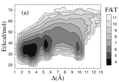
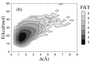
Figure 1: Free energy $F(\Delta,E)=-kT\ln P(\Delta,E)$ at $T=273$ K for (a) the $\beta$-hairpin and (b) the F${}_{\mbox{{\small s}}}$ peptide. $E$ is energy and $\Delta$ denotes rmsd from the native $\beta$-hairpin and an ideal $\alpha$-helix, respectively, calculated over all non-hydrogen atoms (a backbone rmsd would be unable to distinguish the two possible $\beta$-hairpin topologies).

Besides its global minimum, $F(\Delta,E)$ exhibits two local minima (see Fig. 1a), one corresponding to a $\beta$-hairpin with the non-native topology ($\Delta\approx 5$ Å), and the other to an $\alpha$-helix ($\Delta\approx 10$ Å). A closer examination of structures from the two $\beta$-hairpin minima reveals that the C_β-C_β distances for Tyr45-Phe52 and Trp43-Val54 tend to be smaller in the non-native topology than in the native one. This is important because it makes it sterically difficult to achieve a proper contact between the aromatic side chains of Tyr45 and Phe52 in the non-native topology. As a result, this topology is hydrophobically disfavored. This is the main reason why the model indeed favors the native topology over the non-native one.

We now turn to the melting behavior of the $\beta$-hairpin. By studying tryptophan fluorescence (Trp43), Muñoz et al. [6] found that the unfolding of this peptide with increasing temperature shows two-state character, with parameters $T_{\mbox{{\scriptsize m}}}=297$ K and $\Delta E=11.6$ kcal/mol, $T_{\mbox{{\scriptsize m}}}$ and $\Delta E$ being the melting temperature and energy change, respectively. To study the character of the melting transition in our model, we monitor the hydrophobicity energy $E_{\mbox{{\scriptsize hp}}}$, a simple observable we expect to be strongly correlated with Trp43 fluorescence. Following Muñoz et al. [6], we fit our data for $E_{\mbox{{\scriptsize hp}}}$ to a first-order two-state model. To reduce the number of parameters of the fit, $T_{\mbox{{\scriptsize m}}}$ is held fixed, at the specific heat maximum (data not shown). The fit turns out not to be perfect, with a $\chi^{2}/{\rm dof}$ of 4.5. The deviations from the fitted curve are nevertheless small, as can be seen from Fig. 2a; they can be detected only because the statistical errors are very small ($\sim 0.1$ %) at the highest temperatures. To further illustrate this point, we assign each data point an artifical uncertainty of 1 %, an error size that is not uncommon for experimental data. With these errors, the same type of fit yields a $\chi^{2}/$dof of 0.3, which confirms that the data indeed to a good approximation show two-state behavior. Our fitted value of $\Delta E$ is $9.3\pm 0.3$ kcal/mol, which implies that the temperature dependence of the model is comparable to experimental data [6].

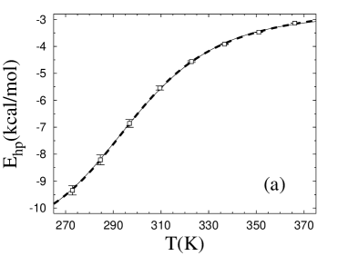
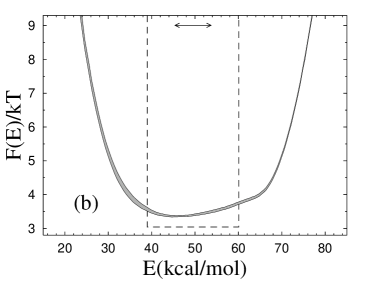
Figure 2: Unfolding of the $\beta$-hairpin sequence. (a) Temperature dependence of the hydrophobicity energy $E_{\mbox{{\scriptsize hp}}}$ (see Eq. 8). The solid and dashed curves (essentially coinciding) are fits of the data to the two-state expression $E_{\mbox{{\scriptsize hp}}}=(E_{\mbox{{\scriptsize hp}}}^{\mbox{{\scriptsize u}}}+KE_{\mbox{{\scriptsize hp}}}^{\mbox{{\scriptsize f}}})/(1+K)$ and the square-well model (see text), respectively. The effective equilibrium constant $K$ is assumed to have the first-order form $K=\exp[(1/kT-1/kT_{\mbox{{\scriptsize m}}})\Delta E]$. Both fits have three free parameters, whereas $T_{\mbox{{\scriptsize m}}}=297$ K is held fixed. (b) Free-energy profile $F(E)=-kT\ln P(E)$ at $T=T_{\mbox{{\scriptsize m}}}$, obtained by reweighting [34] the data at a simulated $T$ close to $T_{\mbox{{\scriptsize m}}}$. The shaded band is centered around the expected value and shows statistical $1\sigma$ errors. The double-headed arrow indicates $\Delta E$ of the two-state fit. The dashed line shows $F(E)$ for the square-well fit.

Several groups have simulated the same $\beta$-hairpin using atomic models with implicit [7, 8, 4] or explicit [9, 10, 11, 12] solvent. Many of these groups studied the melting behavior of the $\beta$-hairpin, but the temperature dependence they found was too weak, as was pointed out by Zhou et al. [12]. In fact, in all these studies, there was a significant $\beta$-hairpin population at temperatures of 400 K and above. Another important difference between at least some of these models [8, 10, 11] and ours, is that in our model there is no clear free-energy minimum corresponding to a hydrophobically collapsed state with few or no hydrogen bonds. A local free-energy minimum with helical content was found in one of these studies [11], but not in the others. Such a minimum exists in our model (see Fig. 1a), but the helix population is low.

In spite of its minimalistic potential, our model is able to make $\alpha$-helices too. To show this, we consider the $\alpha$-helical so-called F${}_{\mbox{{\small s}}}$ peptide, which has been extensively studied both experimentally [13, 14, 15, 16] and theoretically [33]. This 21-amino acid peptide is given by AAAAA(AAARA)₃A, where A is Ala and R is Arg. Using exactly the same model as before, with unchanged parameters, we find that the F${}_{\mbox{{\small s}}}$ sequence does make an $\alpha$-helix. This can be seen from Fig. 1b, which shows the free energy $F(\Delta,E)$ at $T=273$ K, $\Delta$ this time denoting rmsd from an ideal $\alpha$-helix. $F(\Delta,E)$ has only one significant minimum, which indeed is helical. The melting behavior of this sequence is illustrated in Fig. 3a, which shows the temperature dependence of the hydrogen-bond energy. Data are again quite well described by a first-order two-state model; the $\chi^{2}/{\rm dof}$ for the fit is 20.5 and would be 1.7 if the errors were 1 %. Our fitted value of $\Delta E$ is $16.1\pm 0.9$ kcal/mol for F${}_{\mbox{{\small s}}}$, which may be compared to the result $\Delta E=12\pm 2$ kcal/mol obtained by a two-state fit of infrared (IR) spectroscopy data [15]. As in the $\beta$-hairpin analysis, $T_{\mbox{{\scriptsize m}}}$ is determined from the specific heat maximum (data not shown). For F${}_{\mbox{{\small s}}}$, we obtain $T_{\mbox{{\scriptsize m}}}=310$ K, which may be compared to the values $T_{\mbox{{\scriptsize m}}}=303$, 308 K and $T_{\mbox{{\scriptsize m}}}=334$ K obtained by circular dichroism (CD) [14, 16] and IR spectroscopy [15], respectively. Let us stress that $T_{\mbox{{\scriptsize m}}}$ for F${}_{\mbox{{\small s}}}$ is a prediction of the model; the energy scale of the model is set using $T_{\mbox{{\scriptsize m}}}$ for the $\beta$-hairpin and then left unchanged in our study of F${}_{\mbox{{\small s}}}$.

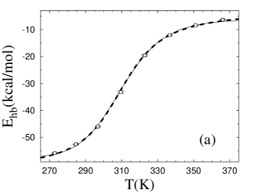
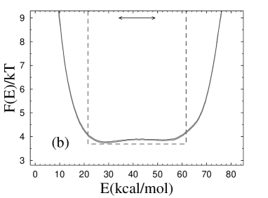
Figure 3: Unfolding of the F${}_{\mbox{{\small s}}}$ sequence. (a) Temperature dependence of the hydrogen-bond energy $E_{\mbox{{\scriptsize hb}}}$ (see Eq. 3), with the same two types of fit as in Fig. 2a (same symbols). (b) Free-energy profile $F(E)=-kT\ln P(E)$ at $T=T_{\mbox{{\scriptsize m}}}$. Same symbols as in Fig. 2b.

The two-state fits shown in Figs. 2a and 3a are based on a first-order expression for the free energies of the two coexisting phases. The fits look good and can be improved by including higher order terms, which may give the impression that the behaviors of these systems can be fully understood in terms of a two-state model. However, the two-state picture is far from perfect. This can be seen from the free-energy profiles $F(E)$ shown in Figs. 2b and 3b, which lack a clear bimodal shape. Clearly, this renders the parameters of a two-state model, such as $\Delta E$, ambiguous. The analysis of these systems therefore shows that the results of a two-state fit must be interpreted with care. Given the actual shapes of $F(E)$, it is instructive to perform an alternative fit of the data in Figs. 2a and 3a, based on the assumptions that 1) $F(E)$ has the shape of a square well of width $\Delta E_{\mbox{{\scriptsize sw}}}$ at $T=T_{\mbox{{\scriptsize m}}}$, and that 2) the observable analyzed varies linearly with $E$. These square-well fits are shown in Figs. 2a and 3a, and the corresponding free-energy profiles $F(E)$ (at $T=T_{\mbox{{\scriptsize m}}}$) are indicated in Figs. 2b and 3b. The square-well fits are somewhat better than the two-state fits. However, the fitted curves are strikingly similar, given the large difference between the underlying energy distributions. This shows that it is very hard to draw conclusions about the free-energy profile $F(E)$ from the temperature dependence of a single observable.

From Figs. 2b and 3b it can also be seen that the energy change $\Delta E$ obtained from the two-state fit is considerably smaller than the width of the energy distribution, which indicates that $\Delta E$ is smaller than the calorimetric energy change $\Delta E_{\mbox{{\scriptsize cal}}}$. Scholtz et al. [35] determined $\Delta E_{\mbox{{\scriptsize cal}}}$ experimentally for an Ala-based helical peptide with 50 amino acids, and obtained a value of 1.3 kcal/mol per amino acid. This value corresponds to a $\Delta E_{\mbox{{\scriptsize cal}}}$ of 27.3 kcal/mol for the F${}_{\mbox{{\small s}}}$ peptide. Comparing model results for $\Delta E_{\mbox{{\scriptsize cal}}}$ with experimental data is not straightforward, due to uncertainties about what the relevant baseline subtractions are [36, 37, 38]. If we ignore baseline subtractions and simply define $\Delta E_{\mbox{{\scriptsize cal}}}$ as the energy change between the highest and lowest temperatures studied, we obtain $\Delta E_{\mbox{{\scriptsize cal}}}=45.6\pm 0.1$ kcal/mol for F${}_{\mbox{{\small s}}}$, which is larger than the value of Scholtz et al. [35]. To get an idea of how much this result can be affected by a baseline subtraction, a fit of our specific heat data is performed, to a two-state expression supplemented with a baseline linear in $T$. The fit function is $C_{\mbox{{\scriptsize v}}}=\Delta E_{\mbox{{\scriptsize cal}}}(1+K)^{-2}\frac{dK}{dT}+c_{0}+c_{1}(T-T_{\mbox{{\scriptsize m}}})$, where $c_{0}$ and $c_{1}$ are baseline parameters and $K=\exp[(1/kT-1/kT_{\mbox{{\scriptsize m}}})\Delta E]$. With $\Delta E_{\mbox{{\scriptsize cal}}}$, $\Delta E$, $c_{0}$, $c_{1}$ and $T_{\mbox{{\scriptsize m}}}$ as free parameters, this fit gives $\Delta E_{\mbox{{\scriptsize cal}}}=34.0\pm 1.0$ kcal/mol ($\chi^{2}/{\rm dof}=5.2$), which is considerably closer to the value of Scholtz et al. [35]. It may be worth noting that the corresponding fit without baseline subtraction is much poorer ($\chi^{2}/{\rm dof}\sim 300$). From these calculations, we conclude that the model may overestimate $\Delta E_{\mbox{{\scriptsize cal}}}$, but it is not evident that the deviation is statistically significant, due to theoretical as well as experimental uncertainties.

The melting behavior of helical peptides is often analyzed using the Zimm-Bragg [39] or Lifson-Roig [40] models, which for large chain lengths are very different from the two-state model considered above. Our results for the F${}_{\mbox{{\small s}}}$ peptide are, nevertheless, quite well described by these models too. In fact, a fit of the helix content as a function of temperature to the Lifson-Roig model gives a $\chi^{2}/{\rm dof}$ similar to that for the two-state fit above. Our fitted Lifson-Roig parameters are $v=0.016\pm 0.009$ and $w(T=273\,{\rm K})=1.86\pm 0.25$, corresponding to the Zimm-Bragg parameters $\sigma=0.0003\pm 0.0003$ and $s(T=273\,{\rm K})=1.83\pm 0.25$ [41]. In this fit the temperature dependence of $w$ is given by a first-order two-state expression, whereas $v$ is held constant. The energy change $\Delta E_{w}$ has a fitted value of $1.33\pm 0.17$ kcal/mol. The statistical uncertainties on $v$ and $\sigma$ are large because the chain is small, which makes the dependence on these parameters weak. Thompson et al. [16] performed a Zimm-Bragg analysis of CD data for F${}_{\mbox{{\small s}}}$, using the single-sequence approximation. Assuming a value of $\Delta E_{s}=1.3$ kcal/mol for the energy change associated with helix propagation, they obtained a $\sigma$ of 0.0012.

Our kinetic simulations of the two peptides are performed at their respective melting temperatures, $T_{\mbox{{\scriptsize m}}}$. Starting from equilibrium conformations at $T=366$ K, we study the relaxation of ensemble averages under Monte Carlo dynamics (see Section 2.2). The ensemble consists of 1500 independent runs for each peptide. In Fig. 4, we show the “time” evolution of $\delta O(t)=O(t)-\langle O\rangle$, where $O(t)$ is an ensemble average after $t$ Monte Carlo steps, $\langle O\rangle$ is the corresponding equilibrium average, and the observable $O$ is $E_{\mbox{{\scriptsize hp}}}$ for the $\beta$-hairpin and $E_{\mbox{{\scriptsize hb}}}$ for F${}_{\mbox{{\small s}}}$ (same observables as in the thermodynamic calculations). Ignoring a brief initial period of rapid change, we find that the data, for both peptides, are fully consistent with single-exponential relaxation ($\chi^{2}/{\rm dof}\sim 1$), although the interval over which the signal $\delta O(t)$ can be followed is small in units of the relaxation time, especially for the $\beta$-hairpin. Nevertheless, assuming the single-exponential behavior to be correct, a statistically quite accurate determination of the relaxation times can be obtained. The fitted relaxation time is approximately a factor of 5 larger for the $\beta$-hairpin than for F${}_{\mbox{{\small s}}}$. The corresponding factor is around 30 for experimental data [6, 15, 16]. A closer look at the $\beta$-hairpin data shows that the hydrophobic cluster and the hydrogen bonds, on average, form nearly simultaneously in our model. This is in agreement with the results of Zhou et al. [12], and in disagreement with the folding mechanism of Pande and Rokhsar [10] in which the collapse occurs before the hydrogen bonds form.

Figure 4: Monte Carlo relaxation of ensemble averages at $T=T_{\mbox{{\scriptsize m}}}$ for the $\beta$-hairpin and the F${}_{\mbox{{\small s}}}$ peptide. The deviation $\delta O(t)$ from the equilibrium average (see text) is plotted against the number of elementary Monte Carlo steps, $t$. Straight lines are $\chi^{2}$ fits of the data to a single exponential. Data for $t>15\cdot 10^{6}$ are omitted for F${}_{\mbox{{\small s}}}$ due to large statistical errors.

The two peptides studied in this paper make unusually clear-cut $\alpha$- and $\beta$-structure, respectively. It is clear that refinements of the interaction potential will be required in order to obtain an equally good description of more general sequences. One interesting refinement would be to make the strength of the hydrogen bonds context-dependent, that is dependent on whether the hydrogen bond is internal or exposed. This is probably needed in order for the model to capture, for example, the difference between the Ala-based F${}_{\mbox{{\small s}}}$ peptide and pure polyalanine. In fact, it has been argued [33, 42] that a major reason why F${}_{\mbox{{\small s}}}$ is a strong helix maker is that the Arg side chains shield the backbone from water and thereby make the hydrogen bonds stronger. The hydrogen bonds of a polyalanine helix lack this protection. In our model, the hydrogen bonds are context-independent, which could make polyalanine too helical. Although a direct comparison with experimental data is impossible due to its poor water solubility, simulations of polyalanine with 21 amino acids, A₂₁, seem to confirm this. For A₂₁, we obtain a helix content of about 80 % at $T=273$ K, which is what we find for F${}_{\mbox{{\small s}}}$ too. Using a modified version of the Cornell et al. force field [43], García and Sanbonmatsu [33] obtained a helix content of 34 % at $T=275$ K for A₂₁; the unmodified force field was found [33] to give a value similar to ours at this temperature (but very different from ours at higher $T$). Our estimate that F${}_{\mbox{{\small s}}}$ is $\sim$ 80 % helical at $T=273$ K is consistent with experimental data [13, 16].

We also looked at two other helical peptides. The first of these is the Ala-based 16-amino acid peptide (AEAAK)₃A, where E is Glu and K is Lys. By CD, Marqusee and Baldwin [44] found this peptide to be $\sim$ 50 % helical at $T=274$ K. In our model the corresponding value turns out to be $\sim$ 70 %. Our last example is the 38–59-fragment of the B domain of staphylococcal protein A (PDB code 1BDD). This is a more general, not Ala-based sequence, containing three hydrophobic Leu. By CD, Bai et al. [45] obtained a helix content of $\sim$ 30 % at pH 5.2 and $T=278$ K for this fragment. In our model we obtain a helix content of $\sim$ 20 % at this temperature. So, the model predicts helix contents that are in approximate agreement with experimental data for F${}_{\mbox{{\small s}}}$, (AEAAK)₃A as well as the protein A fragment.

4 Summary and Outlook

We have developed and explored a protein model that combines an all-atom representation of the amino acid chain with a minimalistic sequence-based potential. The strength of the model is the simplicity of the potential, which at the same time, of course, means that there are many interesting features of real proteins that the model is unable to capture. One advantage of the model is that the calibration of parameters, which any model needs, becomes easier to carry out with fewer parameters to tune.

When calibrating the model, our goal was to ensure that, without resorting to parameter changes, our two sequences made a $\beta$-hairpin with the native topology and an $\alpha$-helix, respectively, which was not an easy task. Once this goal had been achieved, our thermodynamic and kinetic measurements were carried out without any further fine-tuning of the potential. Therefore, it is hard to believe that the generally quite good agreement between our thermodynamic results and experimental data is accidental. A more plausible explanation of the agreement is that the thermodynamics of these two sequences indeed are largely governed by backbone hydrogen bonding and hydrophobic collapse forces, as assumed by the model. The requirement that the two sequences make the desired structures is then sufficient to quite accurately determine the strengths of these two terms.

The main results of our calculations can be summarized as follows.

• Our thermodynamic simulations show first of all that the two sequences studied indeed make a $\beta$-hairpin with the native topology and an $\alpha$-helix, respectively. The main reason why the model favors the native topology over the non-native one for the $\beta$-hairpin, is that the formation of the hydrophobic cluster is sterically difficult to accomplish in the non-native topology. The melting curves obtained for the two peptides are in reasonable agreement with experimental data, and can to a good approximation be described by a simple two-state model.

• A two-state description of the thermodynamic behavior is, nevertheless, found to be an oversimplification for both peptides, as can be seen from the energy distributions. Given that the systems are small and fluctuations therefore relatively large, this is maybe not surprising. What is striking is how difficult it is to detect these deviations from two-state behavior when studying the temperature dependence of a single observable.

• The results of our Monte Carlo-based kinetic runs at the respective melting temperatures are, for both peptides, consistent with single-exponential relaxation, and the relaxation time is found to be larger for the $\beta$-hairpin than for F${}_{\mbox{{\small s}}}$.

Extending these calculations to larger chains will impose new conditions on the interaction potential, and thereby make it possible (and necessary) to refine it. Two interesting refinements would be to make the treatment of charged side chains and side-chain hydrogen bonds less crude and to introduce a mechanism for screening of hydrogen bonds [33, 46, 42, 47]. Computationally, there is room for extending the calculations. In fact, simulating the thermodynamics of a chain with about 20 amino acids, with high statistics, does not take more than a few days on a standard desktop computer, in spite of the detailed geometry of the model. This gives us hope to be able to look into the free-energy landscape and two-state character of small proteins in a not too distant future.

Acknowledgments

We thank Giorgio Favrin for stimulating discussions and help with computers. This work was in part supported by the Swedish Foundation for Strategic Research and the Swedish Research Council.

References

- [1] Shimada, J. & Shakhnovich, E.I. (2002) Proc. Natl. Acad. Sci. USA 99, 11175–11180.
- [2] Clementi, C., García, A.E. & Onuchic, J.N. (2003) J. Mol. Biol. 326, 933–954.
- [3] Gō, N. & Abe, H. (1981) Biopolymers 20, 991–1011.
- [4] Kussell, E., Shimada, J. & Shakhnovich, E.I. (2002) Proc. Natl. Acad. Sci. USA 99, 5343–5348.
- [5] Blanco, F.J., Rivas, G. & Serrano, L. (1994) Nat. Struct. Biol. 1, 584–590.
- [6] Muñoz, V., Thompson, P.A., Hofrichter, J. & Eaton, W.A. (1997) Nature 390, 196–199.
- [7] Dinner, A.R., Lazaridis, T. & Karplus, M. (1999) Proc. Natl. Acad. Sci. USA 96, 9068–9073.
- [8] Zagrovic, B., Sorin, E.J. & Pande, V. (2001) J. Mol. Biol. 313, 151–169.
- [9] Roccatano, D., Amadei, A., Di Nola, A. & Berendsen, H.J.C. (1999) Protein Sci. 8, 2130–2143.
- [10] Pande, V.S. & Rokhsar, D.S. (1999) Proc. Natl. Acad. Sci. USA 96, 9062–9067.
- [11] García, A.E. & Sanbonmatsu, K.Y. (2001) Proteins 42, 345–354.
- [12] Zhou, R., Berne, B.J. & Germain, R. (2001) Proc. Natl. Acad. Sci. USA 98, 14931–14936.
- [13] Lockhart, D.J. & Kim, P.S. (1992) Science 257, 947–951.
- [14] Lockhart, D.J. & Kim, P.S. (1993) Science 260, 198–202.
- [15] Williams, S., Causgrove, T.P., Gilmanshin, R., Fang, K.S., Callender, R.H., Woodruff, W.H. & Dyer, R.B. (1996) Biochemistry 35, 691–697.
- [16] Thompson, P.A., Eaton, W.A. & Hofrichter, J. (1997) Biochemistry 36, 9200–9210.
- [17] Irbäck, A., Sjunnesson, F. & Wallin, S. (2000) Proc. Natl. Acad. Sci. USA 97, 13614–13618.
- [18] Irbäck, A., Sjunnesson, F. & Wallin, S. (2001) J. Biol. Phys. 27, 169–179.
- [19] Favrin, G., Irbäck, A. & Wallin, S. (2002) Proteins 47, 99–105.
- [20] Bernstein, F.C., Koetzle, T.F., Williams, G.J.B., Meyer, E.F., Brice, M.D., Rodgers, J.R., Kennard, O., Shimanouchi, T. & Tasumi, M. (1977) J. Mol. Biol. 112, 535–542.
- [21] Tsai, J., Taylor, R., Chothia, C. & Gerstein, M. (1999) J. Mol. Biol. 290, 253–266.
- [22] Miyazawa, S. & Jernigan, R.L. (1996) J. Mol. Biol. 256, 623–644.
- [23] Li, H., Tang, C. & Wingreen, N.S. (1997) Phys. Rev. Lett. 79, 765–768.
- [24] Lyubartsev, A.P., Martsinovski, A.A., Shevkunov, S.V. & Vorontsov-Velyaminov, P.N. (1992) J. Chem. Phys. 96, 1776–1783.
- [25] Marinari, E. & Parisi, G. (1992) Europhys. Lett. 19, 451–458.
- [26] Irbäck, A. & Potthast, F. (1995) J. Chem. Phys. 103, 10298–10305.
- [27] Metropolis, N., Rosenbluth, A.W., Rosenbluth, M.N., Teller, A.H. & Teller, E. (1953) J. Chem. Phys. 21, 1087–1092.
- [28] Lal, M. (1969) Mol. Phys. 17, 57–64.
- [29] Favrin, G., Irbäck, A. & Sjunnesson, F. (2001) J. Chem. Phys. 114, 8154–8158.
- [30] Press, W.H., Flannery, B.P., Teukolsky, S.A. & Vetterling, W.T. (1992) Numerical Recipes in C: The Art of Scientific Computing, (Cambridge University Press, Cambridge).
- [31] Gronenborn, A.M., Filpula, D.R., Essig, N.Z., Achari, A., Whitlow, M., Wingfield, P.T. & Clore, G.M. (1991) Science 253, 657–661.
- [32] Kobayashi, N., Honda, S., Yoshii, H. & Munekata, E. (2000) Biochemistry 39, 6564–6571.
- [33] García, A.E. & Sanbonmatsu, K.Y. (2002) Proc. Natl. Acad. Sci. USA 99, 2782–2787.
- [34] Ferrenberg, A.M. & Swendsen R.H. (1988) Phys. Rev. Lett. 61, 2635–2638, and erratum (1989) 63, 1658, and references given in the erratum.
- [35] Scholtz, J.M., Marqusee, S., Baldwin, R.L., York, E.J., Stewart, J.M., Santaro, M. & Bolen, D.W. (1991) Proc. Natl. Acad. Sci. USA 88, 2854–2858.
- [36] Zhou, Y., Hall, C.K. & Karplus, M. (1999) Protein Sci. 8, 1064–1074.
- [37] Chan, H.S. (2000) Proteins 40, 543–571.
- [38] Kaya, H. & Chan, H.S. (2000) Proteins 40, 637–661.
- [39] Zimm, B.H. & Bragg, J.K. (1959) J. Chem. Phys. 31, 526–535.
- [40] Lifson, S. & Roig, A. (1960) J. Chem. Phys. 34, 1963–1974.
- [41] Qian, H. & Schellman, J.A. (1992) J. Phys. Chem. 96, 3987–3994.
- [42] Vila, J.A., Ripoll, D.R. & Scheraga, H.A. (2000) Proc. Natl. Acad. Sci. USA 97, 13075–13079.
- [43] Cornell, W.D, Cieplak, P, Bayly, C.I., Gould, I.R, Merz, K.M., Ferguson, D.M., Spellmeyer, D.C., Fox, T., Caldwell, J.W. & Kollman, P.A. (1995) J. Am. Chem. Soc. 117, 5179–5197.
- [44] Marqusee, S. & Baldwin, R.L. (1987) Proc. Natl. Acad. Sci. USA 84, 8898–8902.
- [45] Bai, Y., Karimi, A., Dyson, H.J. & Wright, P.E. (1997) Protein Sci. 6, 1449–1457.
- [46] Takada, S., Luthey-Schulten, Z. & Wolynes, P.G. (1999) J. Chem. Phys. 110, 11616–11629.
- [47] Guo, C., Cheung, M.S., Levine, H. & Kessler, D.A. (2002) J. Chem. Phys. 116, 4353–4365.