Abstract:
We present a Monte Carlo study of a model protein with 54 amino acids that folds directly to its native three-helix-bundle state without forming any well-defined intermediate state. The free-energy barrier separating the native and unfolded states of this protein is found to be weak, even at the folding temperature. Nevertheless, we find that melting curves to a good approximation can be described in terms of a simple two-state system, and that the relaxation behavior is close to single exponential. The motion along individual reaction coordinates is roughly diffusive on timescales beyond the reconfiguration time for an individual helix. A simple estimate based on diffusion in a square-well potential predicts the relaxation time within a factor of two.

Keywords: protein folding, folding thermodynamics, folding kinetics, two-state system, diffusive dynamics, Monte Carlo simulation.

1 Introduction

In a landmark paper in 1991, Jackson and Fersht [1] demonstrated that chymotrypsin inhibitor 2 folds without significantly populating any meta-stable intermediate state. Since then, it has become clear that this protein is far from unique; the same behavior has been observed for many small single-domain proteins [2]. It is tempting to interpret the apparent two-state behavior of these proteins in terms of a simple free-energy landscape with two minima separated by a single barrier, where the minima represent the native and unfolded states, respectively. If the barrier is high, this picture provides an explanation of why the folding kinetics are single exponential, and why the folding thermodynamics show two-state character.

However, it is well-known that the free-energy barrier, $\Delta F$, is not high for all these proteins. In fact, assuming the folding time $\tau_{\mbox{{\scriptsize f}}}$ to be given by $\tau_{\mbox{{\scriptsize f}}}=\tau_{0}\exp(\Delta F/kT)$ with $\tau_{0}\sim 1\,\mu s$ [3], it is easy to find examples of proteins with $\Delta F$ values of a few $kT$  [2] ($k$ is Boltzmann’s constant and $T$ the temperature). It should also be mentioned that Garcia-Mira et al. [4] recently found a protein that appears to fold without crossing any free-energy barrier.

Suppose the native and unfolded states coexist at the folding temperature and that there is no well-defined intermediate state, but that a clear free-energy barrier is missing. What type of folding behavior should one then expect? In particular, would such a protein, due to the lack of a clear free-energy barrier, show easily detectable deviations from two-state thermodynamics and single-exponential kinetics? Here we investigate this question based on Monte Carlo simulations of a designed three-helix-bundle protein [5, 6, 7].

Our study consists of three parts. First, we investigate whether or not melting curves for this model protein show two-state character. Second, we ask whether the relaxation behavior is single exponential or not, based on ensemble kinetics at the folding temperature. Third, inspired by energy-landscape theory (for a recent review, see Refs. [8, 9]), we try to interpret the folding dynamics of this system in terms of simple diffusive motion in a low-dimensional free-energy landscape.

2 Model and Methods

2.1 The Model

Simulating atomic models for protein folding remains a challenge, although progress is currently being made in this area [10, 11, 12, 13, 14, 15, 16]. Here, for computational efficiency, we consider a reduced model with 5–6 atoms per amino acid [5], in which the side chains are replaced by large C_β atoms. Using this model, we study a designed three-helix-bundle protein with 54 amino acids.

The model has the Ramachandran torsion angles $\phi_{i}$, $\psi_{i}$ as its degrees of freedom, and is sequence-based with three amino acid types: hydrophobic (H), polar (P) and glycine (G). The sequence studied consists of three identical H/P segments with 16 amino acids each (PPHPPHHPPHPPHHPP), separated by two short GGG segments [17, 18]. The H/P segment is such that it can make an $\alpha$-helix with all the hydrophobic amino acids on the same side.

The interaction potential

$$E=E_{\mbox{{\scriptsize loc}}}+E_{\mbox{{\scriptsize ev}}}+E_{\mbox{{\scriptsize hb}}}+E_{\mbox{{\scriptsize hp}}}$$ (1)

is composed of four terms. The local potential $E_{\mbox{{\scriptsize loc}}}$ has a standard form with threefold symmetry,

$$E_{\mbox{{\scriptsize loc}}}=\frac{\epsilon_{\phi}}{2}\sum_{i}(1+\cos 3\phi_{i})+\frac{\epsilon_{\psi}}{2}\sum_{i}(1+\cos 3\psi_{i})\,.$$ (2)

The excluded-volume term $E_{\mbox{{\scriptsize ev}}}$ is given by a hard-sphere potential of the form

$$E_{\mbox{{\scriptsize ev}}}=\epsilon_{\mbox{{\scriptsize ev}}}\mathop{{\sum}^{\prime}}_{i<j}\bigg{(}\frac{\sigma_{ij}}{r_{ij}}\bigg{)}^{12}\,,$$ (3)

where the sum runs over all possible atom pairs except those consisting of two hydrophobic C_β. The parameter $\sigma_{ij}$ is given by $\sigma_{ij}=\sigma_{i}+\sigma_{j}+\Delta\sigma_{ij}$, where $\Delta\sigma_{ij}=0.625$ Å for C_βC^′, C_βN and C_βO pairs that are connected by a sequence of three covalent bonds, and $\Delta\sigma_{ij}=0$ Å otherwise. The introduction of the parameter $\Delta\sigma_{ij}$ can be thought of as a change of the local potential.

The hydrogen-bond term $E_{\mbox{{\scriptsize hb}}}$ has the form

$$E_{\mbox{{\scriptsize hb}}}=\epsilon_{\mbox{{\scriptsize hb}}}\sum_{ij}u(r_{ij})v(\alpha_{ij},\beta_{ij})\,,$$ (4)

where the functions $u(r)$ and $v(\alpha,\beta)$ are given by

$$u(r) = 5\bigg{(}\frac{\sigma_{\mbox{{\scriptsize hb}}}}{r}\bigg{)}^{12}-6\bigg{(}\frac{\sigma_{\mbox{{\scriptsize hb}}}}{r}\bigg{)}^{10}$$ (5)

$$v(\alpha,\beta) = \left\{\begin{array}[]{ll}\cos^{2}\alpha\cos^{2}\beta&\ \alpha,\beta>90^{\circ}\\ 0&\ \mbox{otherwise}\end{array}\right.$$ (8)

The sum in Eq. 4 runs over all possible HO pairs, and $r_{ij}$ denotes the HO distance, $\alpha_{ij}$ the NHO angle, and $\beta_{ij}$ the HOC^′ angle. The last term of the potential, the hydrophobicity term $E_{\mbox{{\scriptsize hp}}}$, is given by

$$E_{\mbox{{\scriptsize hp}}}=\epsilon_{\mbox{{\scriptsize hp}}}\sum_{i<j}\bigg{[}\bigg{(}\frac{\sigma_{\mbox{{\scriptsize hp}}}}{r_{ij}}\bigg{)}^{12}-2\bigg{(}\frac{\sigma_{\mbox{{\scriptsize hp}}}}{r_{ij}}\bigg{)}^{6}\,\bigg{]}\,,$$ (9)

where the sum runs over all pairs of hydrophobic C_β.

To speed up the calculations, a cutoff radius $r_{c}$ is used, which is taken to be 4.5 Å for $E_{\mbox{{\scriptsize ev}}}$ and $E_{\mbox{{\scriptsize hb}}}$, and 8 Å for $E_{\mbox{{\scriptsize hp}}}$. Numerical values of all energy and geometry parameters can be found elsewhere [5].

The thermodynamic behavior of this three-helix-bundle protein has been studied before [5, 6]. These studies demonstrated that this model protein has the following properties:

• It does form a stable three-helix bundle, except for a twofold topological degeneracy. These two topologically distinct states both contain three right-handed helices. They differ in how the helices are arranged. If we let the first two helices form a U, then the third helix is in front of the U in one case (FU), and behind the U in the other case (BU). The reason that the model is unable to discriminate between these two states is that their contact maps are effectively very similar [19].

• It makes more stable helices than the corresponding one- and two-helix sequences, which is in accord with the experimental fact that tertiary interactions generally are needed for secondary structure to become stable.

• It undergoes a first-order-like folding transition directly from an expanded state to the three-helix-bundle state, without any detectable intermediate state. At the folding temperature $T_{\mbox{{\scriptsize f}}}$, there is a pronounced peak in the specific heat.

Here we analyze the folding dynamics of this protein in more detail, through an extended study of both thermodynamics and kinetics.

As a measure of structural similarity with the native state, we monitor a parameter $Q$ that we call nativeness (the same as in [5, 6, 7]). To calculate $Q$, we use representative conformations for the FU and BU topologies, respectively, obtained by energy minimization. For a given conformation, we compute the root-mean-square deviations $\delta_{\mbox{\scriptsize FU}}$ and $\delta_{\mbox{\scriptsize BU}}$ from these two representative conformations (calculated over all backbone atoms). The nativeness $Q$ is then obtained as

$$Q=\max\left[\exp\left(-\delta_{\mbox{\scriptsize FU}}^{2}/(10\mbox{\AA})^{2}\right),\,\exp\left(-\delta_{\mbox{\scriptsize BU}}^{2}/(10\mbox{\AA})^{2}\right)\right]\,,$$ (10)

which makes $Q$ a dimensionless number between 0 and 1.

Energies are quoted in units of $kT_{\mbox{{\scriptsize f}}}$, with the folding temperature $T_{\mbox{{\scriptsize f}}}$ defined as the specific heat maximum. In the dimensionless energy unit used in our previous study [5], this temperature is given by $kT_{\mbox{{\scriptsize f}}}=0.6585\pm 0.0006$.

2.2 Monte Carlo Methods

To simulate the thermodynamic behavior of this model, we use simulated tempering [20, 21, 22], in which the temperature is a dynamic variable. This method is chosen in order to speed up the calculations at low temperatures. Our simulations are started from random configurations. The temperatures studied range from $0.95\,T_{\mbox{{\scriptsize f}}}$ to $1.37\,T_{\mbox{{\scriptsize f}}}$.

The temperature update is a standard Metropolis step. In conformation space we use two different elementary moves: first, the pivot move in which a single torsion angle is turned; and second, a semi-local method [23] that works with seven or eight adjacent torsion angles, which are turned in a coordinated manner. The non-local pivot move is included in our calculations in order to accelerate the evolution of the system at high temperatures.

Our kinetic simulations are also Monte Carlo-based, and only meant to mimic the time evolution of the system in a qualitative sense. They differ from our thermodynamic simulations in two ways: first, the temperature is held constant; and second, the non-local pivot update is not used, but only the semi-local method [23]. This restriction is needed in order to avoid large unphysical deformations of the chain.

Statistical errors on thermodynamic results are obtained by jackknife analysis [24] of results from ten or more independent runs, each containing several folding/unfolding events. All errors quoted are 1$\sigma$ errors. Statistical errors on relaxation times are difficult to determine due to uncertainties about where the large-time behavior sets in and are therefore omitted. We estimate that the uncertainties on our calculated relaxation times are about 10%. The statistical errors on the results obtained by numerical solution of the diffusion equation are, however, significantly smaller than this.

All fits of data discussed below are carried out by using a Levenberg-Marquardt procedure [25].

2.3 Analysis

Melting curves for proteins are often described in terms of a two-state picture. In the two-state approximation, the average of a quantity $X$ at temperature $T$ is given by

$$X(T)=\frac{X_{\mbox{\scriptsize u}}+X_{\mbox{\scriptsize n}}K(T)}{1+K(T)}\,,$$ (11)

where $K(T)=P_{\mbox{\scriptsize n}}(T)/P_{\mbox{\scriptsize u}}(T)$, $P_{\mbox{\scriptsize n}}(T)$ and $P_{\mbox{\scriptsize u}}(T)$ being the populations of the native and unfolded states, respectively. Likewise, $X_{\mbox{\scriptsize n}}$ and $X_{\mbox{\scriptsize u}}$ denote the respective values of $X$ in the native and unfolded states. The effective equilibrium constant $K(T)$ is to leading order given by $K(T)=\exp[(1/kT-1/kT_{\mbox{{\scriptsize m}}})\Delta E]$, where $T_{\mbox{{\scriptsize m}}}$ is the midpoint temperature and $\Delta E$ the energy difference between the two states. With this $K(T)$, a fit to Eq. 11 has four parameters: $\Delta E$, $T_{\mbox{{\scriptsize m}}}$ and the two baselines $X_{\mbox{\scriptsize u}}$ and $X_{\mbox{\scriptsize n}}$.

A simple but powerful method for quantitative analysis of the folding dynamics is obtained by assuming the motion along different reaction coordinates to be diffusive [26, 27]. The folding process is then modeled as one-dimensional Brownian motion in an external potential given by the free energy $F(r)=-kT\ln P_{\mbox{{\scriptsize eq}}}(r)$, where $P_{\mbox{{\scriptsize eq}}}(r)$ denotes the equilibrium distribution of $r$. Thus, it is assumed that the probability distribution of $r$ at time $t$, $P(r,t)$, obeys Smoluchowski’s diffusion equation

$$\frac{\partial P(r,t)}{\partial t}=\frac{\partial}{\partial r}\left[D(r)\left(\frac{\partial P(r,t)}{\partial r}+\frac{P(r,t)}{kT}\frac{\partial F(r)}{\partial r}\right)\right]\,,$$ (12)

where $D(r)$ is the diffusion coefficient.

This picture is not expected to hold on short timescales, due to the projection onto a single coordinate $r$, but may still be useful provided that the diffusive behavior sets in on a timescale that is small compared to the relaxation time. By estimating $D(r)$ and $F(r)$, it is then possible to predict the relaxation time from Eq. 12. Such an analysis has been successfully carried through for a lattice protein [27].

The relaxation behavior predicted by Eq. 12 is well understood when $F(r)$ has the shape of a double well with a clear barrier. In this situation, the relaxation is single exponential with a rate constant given by Kramers’ well-known result [28]. However, this result cannot be applied to our model, in which the free-energy barrier is small or absent, depending on which reaction coordinate is used. Therefore, we perform a detailed study of Eq. 12 for some relevant choices of $D(r)$ and $F(r)$, using analytical as well as numerical methods.

3 Results

3.1 Thermodynamics

In our thermodynamic analysis, we study the five different quantities listed in Table 1. The first question we ask is to what extent the temperature dependence of these quantities can be described in terms of a first-order two-state system (see Eq. 11).

	$\Delta E/kT_{\mbox{{\scriptsize f}}}$	$T_{\mbox{{\scriptsize m}}}/T_{\mbox{{\scriptsize f}}}$
$E$	40.1 $\pm$ 3.3	1.0050 $\pm$ 0.0020
$E_{\mbox{{\scriptsize hb}}}$	41.0 $\pm$ 2.6	1.0024 $\pm$ 0.0017
$E_{\mbox{{\scriptsize hp}}}$	45.4 $\pm$ 3.3	1.0056 $\pm$ 0.0017
$R_{\mbox{{\scriptsize g}}}$	45.7 $\pm$ 3.8	1.0099 $\pm$ 0.0018
$Q$	53.6 $\pm$ 2.1	0.9989 $\pm$ 0.0008

Table 1: Parameters $\Delta E$ and $T_{\mbox{{\scriptsize m}}}$ obtained by fitting results from our thermodynamic simulations to the two-state expression in Eq. 11. This is done individually for each of the quantities in the first column; the energy $E$, the hydrogen-bond energy $E_{\mbox{{\scriptsize hb}}}$, the hydrophobicity energy $E_{\mbox{{\scriptsize hp}}}$, the radius of gyration $R_{\mbox{{\scriptsize g}}}$ (calculated over all backbone atoms), and the nativeness $Q$ (see Eq. 10). The fits are performed using seven data points in the temperature interval $0.95\,T_{\mbox{{\scriptsize f}}}\leq T\leq 1.11\,T_{\mbox{{\scriptsize f}}}$.

Fits of our data to this equation show that the simple two-state picture is not perfect ($\chi^{2}$ per degree of freedom, dof, of $\sim$ 10), but this can be detected only because the statistical errors are very small at high temperatures ($<0.1\%$). In fact, if we assign artifical statistical errors of 1% to our data points, an error size that is not uncommon for experimental data, then the fits become perfect with a $\chi^{2}$/dof close to unity. Fig. 1 shows the temperature dependence of the hydrogen-bond energy $E_{\mbox{{\scriptsize hb}}}$ and the radius of gyration $R_{\mbox{{\scriptsize g}}}$, along with our two-state fits.

Figure 1: Temperature dependence of (a) the hydrogen-bond energy $E_{\mbox{{\scriptsize hb}}}$ and (b) the radius of gyration $R_{\mbox{{\scriptsize g}}}$. The lines are fits to Eq. 11.

Table 1 gives a summary of our two-state fits. In particular, we see that the fitted values of both the energy change $\Delta E$ and the midpoint temperature $T_{\mbox{{\scriptsize m}}}$ are similar for the different quantities. It is also worth noting that the $T_{\mbox{{\scriptsize m}}}$ values fall close to the folding temperature $T_{\mbox{{\scriptsize f}}}$, defined as the maximum of the specific heat. The difference between the highest and lowest values of $T_{\mbox{{\scriptsize m}}}$ is less than 1%. There is a somewhat larger spread in $\Delta E$, but this parameter has a larger statistical error.

So, the melting curves show two-state character, and the fitted parameters $\Delta E$ and $T_{\mbox{{\scriptsize m}}}$ are similar for different quantities. From this it may be tempting to conclude that the thermodynamic behavior of this protein can be fully understood in terms of a two-state system. The two-state picture is, nevertheless, an oversimplification, as can be seen from the shapes of the free-energy profiles $F(E)$ and $F(Q)$. Fig. 2 shows these profiles at $T=T_{\mbox{{\scriptsize f}}}$. First of all, these profiles show that the native and unfolded states coexist at $T=T_{\mbox{{\scriptsize f}}}$, so the folding transition is first-order-like. However, there is no clear free-energy barrier separating the two states; $F(Q)$ exhibits a very weak barrier, $<1\,kT$, whereas $F(E)$ shows no barrier at all. In fact, $F(E)$ has the shape of a square well rather than a double well.

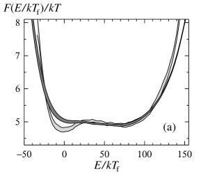
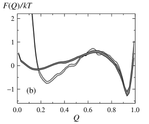
Figure 2: Free-energy profiles at $T=T_{\mbox{{\scriptsize f}}}$ for (a) the energy $E$ and (b) the nativeness $Q$ (dark bands). The light-grey bands show free energies $F_{\mbox{{\scriptsize b}}}$ for block averages (see Eq. 14), using a block size of $\tau_{\mbox{{\scriptsize b}}}=10^{6}$ MC steps. Each band is centered around the expected value and shows statistical 1$\sigma$ errors.

Phase transition terminology is, by necessity, ambiguous for a finite system like this, but if states with markedly different $E$ or $Q$ coexist it does make sense to call the transition first-order-like, even if a free-energy barrier is missing. At a second-order phase transition, the free-energy profile is wide, but the minimum remains unique.

3.2 Kinetics

Our kinetic study is performed at $T=T_{\mbox{{\scriptsize f}}}$. Using Monte Carlo dynamics (see Model and Methods), we study the relaxation of ensemble averages of various quantities. For this purpose, we performed a set of 3000 folding simulations, starting from equilibrium conformations at temperature $T_{0}\approx 1.06\,T_{\mbox{{\scriptsize f}}}$. At this temperature, the chain is extended and has a relatively low secondary-structure content (see Fig. 1).

In the absence of a clear free-energy barrier (see Fig. 2), it is not obvious whether or not the relaxation should be single exponential. To get an idea of what to expect for a system like this, we consider the relaxation of the energy $E$ in a potential $F(E)$ that has the form of a perfect square well at $T=T_{\mbox{{\scriptsize f}}}$. For this idealized $F(E)$ and a constant diffusion coefficient $D(E)$, it is possible to solve Eq. 12 analytically for relaxation at an arbitrary temperature $T$. This solution is given in Appendix A, for the initial condition that $P(E,t=0)$ is the equilibrium distribution at temperature $T_{0}$. Using this result, the deviation from single-exponential behavior can be mapped out as a function of $T_{0}$ and $T$, as is illustrated in Fig. 3. The size of the deviation depends on both $T_{0}$ and $T$, but is found to be small for a wide range of $T_{0}$, $T$ values. This clearly demonstrates that the existence of a free-energy barrier is not a prerequisite to observe single-exponential relaxation.

Figure 3: Level diagram showing the deviation (in %) from a single exponential for diffusion in energy in a square well, based on the exact solution in Appendix A. The system relaxes at temperature $T$, starting from the equilibrium distribution at temperature $T_{0}$. $p$ is defined as $p=(\langle E\rangle-E_{\mbox{\scriptsize n}})/\Delta E_{\mbox{{\scriptsize sw}}}$, where $\langle E\rangle$ is the average energy at temperature $T$, and $E_{\mbox{\scriptsize n}}$ and $\Delta E_{\mbox{{\scriptsize sw}}}$ denote the lower edge and the width, respectively, of the square well. $p$ can be viewed as a measure of the unfolded population at temperature $T$, and is $0.5$ if $T=T_{\mbox{{\scriptsize f}}}$. $p_{0}$ is the the corresponding quantity at temperature $T_{0}$. As a measure of the deviation from a single exponential, we take $\delta_{\max}/\delta E(t_{0})$, where $\delta_{\max}$ is the maximum deviation from a fitted exponential and $\delta E(t_{0})=E(t_{0})-\langle E\rangle$, $E(t_{0})$ being the mean at the smallest time included in the fit, $t_{0}$. Data at times shorter than 1% of the relaxation time were excluded from the fit.

Let us now turn to the results of our simulations. Fig. 4 shows the relaxation of the average energy $E$ and the average nativeness $Q$ in Monte Carlo (MC) time. In both cases, the large-time data can be fitted to a single exponential, which gives relaxation times of $\tau\approx 1.7\cdot 10^{7}$ and $\tau\approx 1.8\cdot 10^{7}$ for $E$ and $Q$, respectively, in units of elementary MC steps. The corresponding fits for the radius of gyration and the hydrogen-bond energy (data not shown) give relaxation times of $\tau\approx 2.1\cdot 10^{7}$ and $\tau\approx 1.8\cdot 10^{7}$, respectively. The fit for the radius of gyration has a larger uncertainty than the others, because the data points have larger errors in this case.

The differences between our four fitted $\tau$ values are small and most probably due to limited statistics for the large-time behavior. Averaging over the four different variables, we obtain a relaxation time of $\tau\approx 1.8\cdot 10^{7}$ MC steps for this protein. The fact that the relaxation times for the hydrogen-bond energy and the radius of gyration are approximately the same shows that helix formation and chain collapse proceed in parallel for this protein. This finding is in nice agreement with recent experimental results for small helical proteins [29].

For $Q$, it is necessary to go to very short times in order to see any significant deviation from a single exponential (see Fig. 4). For $E$, we find that the single-exponential behavior sets in at roughly $\tau/3$, which means that the deviation from this behavior is larger than in the analytical calculation above. On the other hand, for comparisons with experimental data, we expect the behavior of $Q$ to be more relevant than that of $E$. The simulations confirm that the relaxation can be approximately single exponential even if there is no clear free-energy barrier.

Figure 4: Relaxation behavior of the three-helix-bundle protein at the folding temperature $T_{\mbox{{\scriptsize f}}}$, starting from the equilibrium ensemble at $T_{0}\approx 1.06T_{\mbox{{\scriptsize f}}}$. (a) $\delta E(t)=E(t)-\langle E\rangle$ against simulation time $t$, where $E(t)$ is the average $E$ after $t$ MC steps (3000 runs) and $\langle E\rangle$ denotes the equilibrium average (at $T_{\mbox{{\scriptsize f}}}$). (b) Same plot for the nativeness $Q$.

To translate the relaxation time for this protein into physical units, we compare with the reconfiguration time for the corresponding one-helix segment. To that end, we performed a kinetic simulation of this 16-amino acid segment at the same temperature, $T=T_{\mbox{{\scriptsize f}}}$. This temperature is above the midpoint temperature for the one-helix segment, which is $0.95\,T_{\mbox{{\scriptsize f}}}$ [5]. So, the isolated one-helix segment is unstable at $T=T_{\mbox{{\scriptsize f}}}$, but makes frequent visits to helical states with low hydrogen-bond energy, $E_{\mbox{{\scriptsize hb}}}$. To obtain the reconfiguration time, we fitted the large-time behavior of the autocorrelation function for $E_{\mbox{{\scriptsize hb}}}$,

$$C_{\mbox{{\scriptsize hb}}}(t)=\langle E_{\mbox{{\scriptsize hb}}}(t)E_{\mbox{{\scriptsize hb}}}(0)\rangle-\langle E_{\mbox{{\scriptsize hb}}}(0)\rangle^{2}\,,$$ (13)

to an exponential. The exponential autocorrelation time, which can be viewed as a reconfiguration time, turned out to be $\tau_{\mbox{{\scriptsize h}}}\approx 1.0\cdot 10^{6}$ MC steps. This is roughly a factor 20 shorter than the relaxation time $\tau$ for the full three-helix bundle. Assuming the reconfiguration time for an individual helix to be $\sim$ $0.2\,\mu$s [30, 31], we obtain relaxation and folding times of $\sim$ $4\,\mu$s and $\sim$ $8\,\mu$s, respectively, for the three-helix bundle. This is fast but not inconceivable for a small helical protein [2]. In fact, the B domain of staphylococcal protein A is a three-helix-bundle protein that has been found to fold in $<10\,\mu$s, at 37^∘C [32].

3.3 Relaxation-Time Predictions

We now turn to the question of whether the observed relaxation time can be predicted based on the diffusion equation, Eq. 12. For that purpose, we need to know not only the free energy $F(r)$, but also the diffusion coefficient $D(r)$. Socci et al. [27] successfully performed this analysis for a lattice protein that exhibited a relatively clear free-energy barrier. Their estimate of $D(r)$ involved an autocorrelation time for the unfolded state. The absence of a clear barrier separating the native and unfolded states makes it necessary to take a different approach in our case.

The one-dimensional diffusion picture is not expected to hold on short timescales, but only after coarse-graining in time. A computationally convenient way to implement this coarse-graining in time is to study block averages $b(t)$ defined by

$$b(t)=\frac{1}{\tau_{\mbox{{\scriptsize b}}}}\sum_{t\leq s<t+\tau_{\mbox{{\scriptsize b}}}}r(s)\qquad\qquad t=0,\tau_{\mbox{{\scriptsize b}}},2\tau_{\mbox{{\scriptsize b}}},\ldots$$ (14)

where $\tau_{\mbox{{\scriptsize b}}}$ is the block size and $r$ is the reaction coordinate considered. The diffusion coefficient can then be estimated using $D_{\mbox{{\scriptsize b}}}(r)=\langle(\delta b)^{2}\rangle/2\tau_{\mbox{{\scriptsize b}}}$, where the numerator is the mean-square difference between two consecutive block averages, given that the first of them has the value $r$.

In our calculations, we use a block size of $\tau_{\mbox{{\scriptsize b}}}=10^{6}$ MC step, corresponding to the reconfiguration time $\tau_{\mbox{{\scriptsize h}}}$ for an individual helix. We do not expect the dynamics to be diffusive on timescales shorter than this, due to steric traps that can occur in the formation of a helix. In order for the dynamics to be diffusive, the timescale should be such that the system can escape from these traps.

Using this block size, we first make rough estimates of the relaxation times for $E$ and $Q$ based on the result in Appendix A for a square-well potential and a constant diffusion coefficient. These estimates are given by $\tau_{\mbox{{\scriptsize pred,0}}}=\Delta r_{\mbox{{\scriptsize sw}}}^{2}/D_{\mbox{{\scriptsize b}}}\pi^{2}$, where $\Delta r_{\mbox{{\scriptsize sw}}}$ is the width of the potential and $D_{\mbox{{\scriptsize b}}}$ is the average diffusion coefficient.  Our estimates of $\Delta r_{\mbox{{\scriptsize sw}}}$ and $D_{\mbox{{\scriptsize b}}}$ can be found in Table 2, along with the resulting predictions $\tau_{\mbox{{\scriptsize pred,0}}}$. We find that these simple predictions agree with the observed relaxation times $\tau$ within a factor of two.

	$\Delta r_{\mbox{{\scriptsize sw}}}$	$D_{\mbox{{\scriptsize b}}}$	$\tau_{\mbox{{\scriptsize pred,0}}}$	$\tau_{\mbox{{\scriptsize pred}}}$	$\tau$
$E$:	$140kT_{\mbox{{\scriptsize f}}}$	$(9.3\pm 0.2)\cdot 10^{-5}(kT_{\mbox{{\scriptsize f}}})^{2}$	$2.1\cdot 10^{7}$	$1.9\cdot 10^{7}$	$1.7\cdot 10^{7}$
$Q$:	1.0	$(1.00\pm 0.02)\cdot 10^{-8}$	$1.0\cdot 10^{7}$	$0.8\cdot 10^{7}$	$1.8\cdot 10^{7}$

Table 2: The predictions $\tau_{\mbox{{\scriptsize pred,0}}}$ and $\tau_{\mbox{{\scriptsize pred}}}$ (see text) along with the observed relaxation time $\tau$, as obtained from the data in Fig. 4, for the energy $E$ and the nativeness $Q$. $\Delta r_{\mbox{{\scriptsize sw}}}$ is the width of the square-well potential and $D_{\mbox{{\scriptsize b}}}$ is the average diffusion coefficient.

We also did the same calculation for smaller block sizes, $\tau_{\mbox{{\scriptsize b}}}=10^{0}$, $10^{1},\ldots$, $10^{5}$ MC steps. This gave $\tau_{\mbox{{\scriptsize pred,0}}}$ values smaller or much smaller than the observed $\tau$, signaling non-diffusive dynamics. This confirms that for $b(t)$ to show diffusive dynamics, $\tau_{\mbox{{\scriptsize b}}}$ should not be smaller than the reconfiguration time for an individual helix.

Having seen the quite good results obtained by this simple calculation, we now turn to a more detailed analysis, illustrated in Fig. 5a. The block size is the same as before, $\tau_{\mbox{{\scriptsize b}}}=10^{6}$ MC steps, but the space dependence of the diffusion coefficient $D_{\mbox{{\scriptsize b}}}(r)$ is now taken into account, and the potential, $F_{\mbox{{\scriptsize b}}}(r)$, reflects the actual distribution of block averages. The potential $F_{\mbox{{\scriptsize b}}}(r)$, shown in Fig. 2, is not identical to that for the unblocked variables. At a first-order-like transition, we expect free-energy minima to become more pronounced when going to the block variables, provided that the block size $\tau_{\mbox{{\scriptsize b}}}$ is small compared with the relaxation time, because when forming the block variables one effectively integrates out fluctuations about the respective states. The results in Fig. 2 do show this tendency, although the effect is not very strong. Fig. 5b shows the diffusion coefficient $D_{\mbox{{\scriptsize b}}}(E)$, which is largest at intermediate values between the native and unfolded states. The behavior of $D_{\mbox{{\scriptsize b}}}(Q)$ (not shown) is the same in this respect. Hence, there is no sign of a kinetic bottleneck to folding for this protein.

Given $D_{\mbox{{\scriptsize b}}}(r)$ and $F_{\mbox{{\scriptsize b}}}(r)$, we solve Eq. 12 for $P(r,t)$ by using the finite-difference scheme in Appendix B. The initial distribution $P(r,t=0)$ is taken to be the same as in the kinetic simulations. We find that the mean of $P(r,t)$ shows single-exponential relaxation to a good approximation. An exponential fit of these data gives us a new prediction, $\tau_{\mbox{{\scriptsize pred}}}$, for the relaxation time.

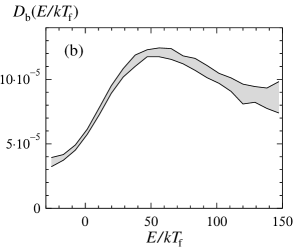
Figure 5: (a) Numerical solution of Eq. 12 with the energy as reaction coordinate. The distribution $P(E,t)$ is shown for $t=0$, $\tau/3$, $\tau$ and $2\tau$ (full lines), where $\tau$ is the relaxation time. The dashed line is the equilibrium distribution. The diffusion coefficient $D_{\mbox{{\scriptsize b}}}(E)$ and the potential $F_{\mbox{{\scriptsize b}}}(E)$ (light-gray band in Fig. 2a) were both determined from numerical simulations, using a block size of $\tau_{\mbox{{\scriptsize b}}}=10^{6}$ MC steps (see Eq. 14). (b) The space dependence of the diffusion coefficient $D_{\mbox{{\scriptsize b}}}(E)$. The band is centered around the expected value and shows the statistical $1\sigma$ error.

From Table 2 it can be seen that the prediction obtained through this more elaborate calculation, $\tau_{\mbox{{\scriptsize pred}}}$, is not better than the previous one, $\tau_{\mbox{{\scriptsize pred,0}}}$, at least not in $Q$, despite that there exists a weak barrier in this coordinate (see Fig. 2b). This means that the barrier in $Q$ is too weak to be important for the relaxation rate. If the underlying diffusion picture, Eq. 12, had been perfect, $\tau_{\mbox{{\scriptsize pred}}}$ would have been equal to $\tau$, as obtained from the kinetic simulations. Our results show that this is not the case. At least in $Q$, there are significant deviations from the behavior predicted by this equation.

If more accurate relaxation time predictions are needed, there are different ways to proceed. One possible way is to simply increase the block size. However, for the calculation to be useful, the block size must remain small compared to the relaxation time. A more interesting possibility is to refine the simple diffusion picture defined by Eq. 12, in which, in particular, non-Markovian effects are ignored. Such effects may indeed affect folding times [33, 9]. Yet another possibility is to use a combination of a few different variables, perhaps $E$ and $Q$, instead of a single reaction coordinate [34, 35, 9]. With a multidimensional representation of the folding process, non-Markovian effects could become smaller.

4 Summary and Discussion

We have analyzed the thermodynamics and kinetics of a designed three-helix-bundle protein, based on Monte Carlo calculations. We found that this model protein shows two-state behavior, in the sense that melting curves to a good approximation can be described by a simple two-state system and that the relaxation behavior is close to single exponential. A simple two-state picture is, nevertheless, an oversimplification, as the free-energy barrier separating the native and unfolded states is weak ($\lesssim 1kT$). The weakness of the barrier implies that a fitted two-state parameter such as $\Delta E$ has no clear physical meaning, despite that the two-state fit looks good.

Reduced [36, 18, 37, 38, 39] and all-atom [40, 41, 11, 10, 14, 42] models for small helical proteins have been studied by many other groups. Most of these studies relied on so-called Gō-type [43] potentials. It should therefore be pointed out that our model is sequence-based.

Using an extended version of this model that includes all atoms, we recently found similar results for two peptides, an $\alpha$-helix and a $\beta$-hairpin [16]. Here the calculated melting curves could be directly compared with experimental data, and a reasonable quantitative agreement was found.

The smallness of the free-energy barrier prompted us to perform an analytical study of diffusion in a square-well potential. Here we studied the relaxation behavior at temperature $T$, starting from the equilibrium distribution at temperature $T_{0}$, for arbitrary $T$ and $T_{0}$. We found that this system shows a relaxation behavior that is close to single exponential for a wide range of $T_{0}$, $T$ values, despite the absence of a free-energy barrier. We also made relaxation-time predictions based on this square-well approximation. Here we took the diffusion coefficient to be constant. It was determined assuming the dynamics to be diffusive on timescales beyond the reconfiguration time for an individual helix. The predictions obtained this way were found to agree within a factor of two with observed relaxation times, as obtained from the kinetic simulations. So, this calculation, based on the two simplifying assumptions that the potential is a square well and that the diffusion coefficient is constant, gave quite good results. A more detailed calculation, in which these two additional assumptions were removed, did not give better results. This shows that the underlying diffusion picture leaves room for improvement.

Our kinetic study focused on the behavior at the folding temperature $T_{\mbox{{\scriptsize f}}}$, where the native and unfolded states, although not separated by a clear barrier, are very different, which makes the folding mechanism transparent. In particular, we found that helix formation and chain collapse could not be separated, which is in accord with experimental data by Krantz et al. [29]. The difference between the native and unfolded states is much smaller at the lowest temperature we studied, $0.95T_{\mbox{{\scriptsize f}}}$, because the unfolded state is much more native-like here. Mayor et al. [44] recently reported experimental results on a three-helix-bundle protein, the engrailed homeodomain [45], including a characterization of its unfolded state. In particular, the unfolded state was found to have a high helix content. This study was performed at a temperature below $0.95T_{\mbox{{\scriptsize f}}}$. It would be very interesting to see what the unfolded state of this protein looks like near $T_{\mbox{{\scriptsize f}}}$. In our model, there is a significant decrease in helix content of the unfolded state as the temperature increases from $0.95T_{\mbox{{\scriptsize f}}}$ to $T_{\mbox{{\scriptsize f}}}$.

It is instructive to compare our results with those of Zhou and Karplus [37], who discussed two folding scenarios for helical proteins, based on a Gō-type C_α model. In their first scenario, folding is fast, without any obligatory intermediate, and helix formation occurs before chain collapse. In the second scenario, folding is slow with an obligatory intermediate on the folding pathway, and helix formation and chain collapse occur simultaneously. The behavior we find does not match any of these two scenarios. In our case, helix formation and chain collapse occur in parallel but folding is nevertheless fast and without any well-defined intermediate state.

Acknowledgments

This work was in part supported by the Swedish Foundation for Strategic Research and the Swedish Research Council.

Appendix A: Diffusion in a square well

Here we discuss Eq. 12 in the situation when the reaction coordinate $r$ is the energy $E$, and the potential $F(E)$ is a square well of width $\Delta E_{\mbox{{\scriptsize sw}}}$ at $T=T_{\mbox{{\scriptsize f}}}$. This means that the equilibrium distribution is given by $P_{\mbox{{\scriptsize eq}}}(E)\propto\exp(-\delta\beta E)$ if $E$ is in the square well and $P_{\mbox{{\scriptsize eq}}}(E)=0$ otherwise, where $\delta\beta=1/kT-1/kT_{\mbox{{\scriptsize f}}}$. Eq. 12 then becomes

$$\frac{\partial P(E,t)}{\partial t}=\frac{\partial}{\partial E}\left[D\left(\frac{\partial P(E,t)}{\partial E}+\delta\beta P(E,t)\right)\right]\,.$$ (15)

For simplicity, the diffusion coefficient is assumed to be constant, $D(E)=D$. The initial distribution $P(E,t=0)$ is taken to be the equilibrium distribution at some temperature $T_{0}$, and we put $\delta\beta_{0}=1/kT_{0}-1/kT_{\mbox{{\scriptsize f}}}$.

By separation of variables, it is possible to solve Eq. 15 with this initial condition analytically for arbitrary values of the initial and final temperatures $T_{0}$ and $T$, respectively. In particular, this solution gives us the relaxation behavior of the average energy. The average energy at time $t$, $E(t)$, can be expressed in the form

$$E(t)=\langle E\rangle+\sum_{k=1}^{\infty}A_{k}{\rm e}^{-t/\tau_{k}}\,,$$ (16)

where $\langle E\rangle$ denotes the equilibrium average at temperature $T$. A straightforward calculation shows that the decay constants in this equation are given by

$$1/\tau_{k}=\frac{D}{\Delta E_{\mbox{{\scriptsize sw}}}^{2}}\left(\pi^{2}k^{2}+{\textstyle\frac{1}{4}}\delta\beta^{2}\Delta E_{\mbox{{\scriptsize sw}}}^{2}\right)$$ (17)

and the expansion coefficients by

$$A_{k}=B_{k}\Delta E_{\mbox{{\scriptsize sw}}}\frac{\pi^{2}k^{2}\left(\delta\beta-\delta\beta_{0}\right)\Delta E_{\mbox{{\scriptsize sw}}}}{\left(\pi^{2}k^{2}+(\delta\beta_{0}-\frac{1}{2}\delta\beta)^{2}\Delta E_{\mbox{{\scriptsize sw}}}^{2}\right)\left(\pi^{2}k^{2}+{\textstyle\frac{1}{4}}\delta\beta^{2}\Delta E_{\mbox{{\scriptsize sw}}}^{2}\right)^{2}}\,,$$ (18)

where

$$B_{k}=\frac{4\delta\beta_{0}\Delta E_{\mbox{{\scriptsize sw}}}}{\sinh{\textstyle\frac{1}{2}}\delta\beta_{0}\Delta E_{\mbox{{\scriptsize sw}}}}\times\left\{\begin{array}[]{ll}\cosh\left(\frac{1}{2}(\delta\beta_{0}-\frac{1}{2}\delta\beta)\Delta E_{\mbox{{\scriptsize sw}}}\right)\cosh\frac{1}{4}\delta\beta\Delta E_{\mbox{{\scriptsize sw}}}&{\rm if}\ k\ {\rm odd}\\ \sinh\left(\frac{1}{2}(\delta\beta_{0}-\frac{1}{2}\delta\beta)\Delta E_{\mbox{{\scriptsize sw}}}\right)\sinh\frac{1}{4}\delta\beta\Delta E_{\mbox{{\scriptsize sw}}}&{\rm if}\ k\ {\rm even}\end{array}\right.$$ (19)

Finally, the equilibrium average is

$$\langle E\rangle=\frac{E_{\mbox{\scriptsize n}}+E_{\mbox{\scriptsize u}}}{2}+\frac{1}{\delta\beta}-\frac{\Delta E_{\mbox{{\scriptsize sw}}}}{2}\coth{\textstyle\frac{1}{2}}\delta\beta\Delta E_{\mbox{{\scriptsize sw}}}\,,$$ (20)

where $E_{\mbox{\scriptsize n}}$ and $E_{\mbox{\scriptsize u}}$ are the lower and upper edges of the square well, respectively.

It is instructive to consider the behavior of this solution when $|\delta\beta-\delta\beta_{0}|\ll 1/\Delta E_{\mbox{{\scriptsize sw}}}$. The expression for the expansion coefficients can then be simplified to

$$A_{k}\approx B_{k}\Delta E_{\mbox{{\scriptsize sw}}}\frac{\pi^{2}k^{2}(\delta\beta-\delta\beta_{0})\Delta E_{\mbox{{\scriptsize sw}}}}{\left(\pi^{2}k^{2}+\frac{1}{4}\delta\beta^{2}\Delta E_{\mbox{{\scriptsize sw}}}^{2}\right)^{3}}$$ (21)

with

$$B_{k}\approx\frac{4\delta\beta_{0}\Delta E_{\mbox{{\scriptsize sw}}}}{\sinh{\textstyle\frac{1}{2}}\delta\beta_{0}\Delta E_{\mbox{{\scriptsize sw}}}}\times\left\{\begin{array}[]{ll}\cosh^{2}\frac{1}{4}\delta\beta\Delta E_{\mbox{{\scriptsize sw}}}&{\rm if}\ k\ {\rm odd}\\ \sinh^{2}\frac{1}{4}\delta\beta\Delta E_{\mbox{{\scriptsize sw}}}&{\rm if}\ k\ {\rm even}\end{array}\right.$$ (22)

Note that $A_{k}$ scales as $k^{2}$ if $k\ll\frac{1}{2\pi}|\delta\beta|\Delta E_{\mbox{{\scriptsize sw}}}$, and as $1/k^{4}$ if $k\gg\frac{1}{2\pi}|\delta\beta|\Delta E_{\mbox{{\scriptsize sw}}}$. Note also that the last factor in $B_{k}$ suppresses $A_{k}$ for even $k$ if $T$ is close to $T_{\mbox{{\scriptsize f}}}$. From these two facts it follows that $|A_{1}|$ is much larger than the other $|A_{k}|$ if $T$ is near $T_{\mbox{{\scriptsize f}}}$. This makes the deviation from a single exponential small.

Appendix B: Numerical solution of the diffusion equation

To solve Eq. 12 numerically for arbitrary $D(r)$ and $F(r)$, we choose a finite-difference scheme of Crank-Nicolson type with good stability properties. To obtain this scheme we first discretize $r$. Put $r_{j}=j\Delta r$, $D_{j}=D(r_{j})$ and $F_{j}=F(r_{j})$, and let ${\bf p}(t)$ be the vector with components $p_{j}(t)=P(r_{j},t)$. Approximating the RHS of Eq. 12 with suitable finite differences, we obtain

$$\frac{d{\bf p}}{dt}={\bf A}{\bf p}(t)\,,$$ (23)

where A is a tridiagonal matrix given by

$$({\bf A}{\bf p}(t))_{j} = \frac{1}{\Delta r^{2}}\left[D_{j+1/2}(p_{j+1}(t)-p_{j}(t))-D_{j-1/2}(p_{j}(t)-p_{j-1}(t))\right]$$ (24)

$$+ \frac{1}{4kT\Delta r^{2}}\left[D_{j+1}p_{j+1}(t)(F_{j+2}-F_{j})-D_{j-1}p_{j-1}(t)(F_{j}-F_{j-2})\right]$$

Let now ${\bf p}^{n}={\bf p}(t_{n})$, where $t_{n}=n\Delta t$. By applying the trapezoidal rule for integration to Eq. 23, we obtain

$${\bf p}^{n+1}-{\bf p}^{n}=\frac{\Delta t}{2}\left({\bf A}{\bf p}^{n}+{\bf A}{\bf p}^{n+1}\right)\,.$$ (25)

This equation can be used to calculate how $P(r,t)$ evolves with time. It can be readily solved for ${\bf p}^{n+1}$ because the matrix ${\bf A}$ is tridiagonal.

References

- [1] Jackson S.E., and A.R. Fersht. 1991. Folding of chymotrypsin inhibitor 2. 1. Evidence for a two-state transition. Biochemistry 30:10428-10435.
- [2] Jackson S.E. 1998. How do small single-domain proteins fold? Fold. Des. 3:R81-R91.
- [3] Hagen S.J., J. Hofrichter, A. Szabo, and W.A. Eaton. 1996. Diffusion-limited contact formation in unfolded cytochrome C: Estimating the maximum rate of protein folding. Proc. Natl. Acad. Sci. USA 93:11615-11617.
- [4] Garcia-Mira M.M., M. Sadqi, N. Fischer, J.M. Sanchez-Ruiz, and V. Mũnoz. 2002. Experimental identification of downhill protein folding. Science 298:2191-2195.
- [5] Irbäck A., F. Sjunnesson, and S. Wallin. 2000. Three-helix-bundle protein in a Ramachandran model. Proc. Natl. Acad. Sci. USA 97:13614-13618.
- [6] Irbäck A., F. Sjunnesson, and S. Wallin. 2001. Hydrogen bonds, hydrophobicity forces and the character of the collapse transition. J. Biol. Phys. 27:169-179.
- [7] Favrin G., A. Irbäck, and S. Wallin. 2002. Folding of a small helical protein using hydrogen bonds and hydrophobicity forces. Proteins 47:99-105.
- [8] Plotkin S.S., and J.N. Onuchic. 2002. Understanding protein folding with energy landscape theory. Part I: Basic concepts. Q. Rev. Biophys. 35:111-167.
- [9] Plotkin S.S., and J.N. Onuchic. 2002. Understanding protein folding with energy landscape theory. Part II: Quantitative aspects. Q. Rev. Biophys. 35:205-286.
- [10] Kussell E., J. Shimada, and E.I. Shakhnovich. 2002. A structure-based method for derivation of all-atom potentials for protein folding. Proc. Natl. Acad. Sci. USA 99:5343-5348.
- [11] Shen M.Y., and K.F. Freed. 2002. All-atom fast protein folding simulations: The villin headpiece. Proteins 49:439-445.
- [12] Zhou R., and B.J. Berne. 2002. Can a continuum solvent model reproduce the free energy landscape of a -hairpin folding in water? Proc. Natl. Acad. Sci. USA 99:12777-12782.
- [13] Shea J.-E., J.N. Onuchic, and C.L. Brooks III. 2002. Probing the folding free energy landscape of the src-SH3 protein domain. Proc. Natl. Acad. Sci. USA 99:16064-16068.
- [14] Zagrovic B., C.D. Snow, M.R. Shirts, and V.S. Pande. 2002. Simulation of folding of a small alpha-helical protein in atomistic detail using worldwide-distributed computing. J. Mol. Biol. 323:927-937.
- [15] Clementi C., A.E. García, and J.N. Onuchic. 2003. Interplay among tertiary contacts, secondary structure formation and side-chain packing in the protein folding mechanism: all-atom representation study of Protein L. J. Mol. Biol. 326:933-954.
- [16] Irbäck A., B. Samuelsson, F. Sjunnesson, and S. Wallin. 2003. Thermodynamics of - and -structure formation in proteins. Preprint submitted to Biophys. J.
- [17] Guo Z., and D. Thirumalai. 1996. Kinetics and thermodynamics of folding of a de novo designed four-helix bundle protein. J. Mol. Biol. 263:323-343.
- [18] Takada S., Z. Luthey-Schulten, and P.G. Wolynes. 1999. Folding dynamics with nonadditive forces: A simulation study of a designed helical protein and a random heteropolymer”, J. Chem. Phys. 110:11616-11628.
- [19] Wallin S., J. Farwer, and U. Bastolla. 2003. Testing similarity measures with continuous and discrete protein models. Proteins 50:144-157.
- [20] Lyubartsev A.P., A.A. Martsinovski, S.V. Shevkunov, and P.N. Vorontsov-Velyaminov. 1992. New approach to Monte Carlo calculation of the free energy: Method of expanded ensembles. J. Chem. Phys. 96:1776-1783.
- [21] Marinari E., and G. Parisi. 1992. Simulated tempering: A new Monte Carlo scheme. Europhys. Lett. 19:451-458.
- [22] Irbäck A., and F. Potthast. 1995. Studies of an off-lattice model for protein folding: Sequence dependence and improved sampling at finite temperature. J. Chem. Phys. 103:10298-10305.
- [23] Favrin G, A. Irbäck, and F. Sjunnesson. 2001. Monte Carlo update for chain molecules: Biased Gaussian steps in torsional space, J. Chem. Phys. 114:8154-8158.
- [24] Miller R.G. 1974. The jackknife - a review. Biometrika 61:1-15.
- [25] Press W.H., B.P. Flannery, S.A. Teukolsky, and W.T. Vetterling. 1992. Numerical Recipes in C: The Art of Scientific Computing. Cambridge University Press, Cambridge.
- [26] Bryngelson J.D., J.N. Onuchic, N.D. Socci, and P.G. Wolynes. 1995. Funnels, pathways, and the energy landscape of protein folding: A synthesis. Proteins 21:167-195.
- [27] Socci N.D., J.N. Onuchic, and P.G. Wolynes. 1996. Diffusive dynamics of the reaction coordinate for protein folding funnels. J. Chem. Phys. 104:5860-5868.
- [28] Kramers H.A. 1940. Brownian motion in a field of force and the diffusion model of chemical reactions. Physica 7:284-304.
- [29] Krantz B.A., A.K. Srivastava, S. Nauli, D. Baker, R.T. Sauer, and T.R. Sosnick. 2002. Understanding protein hydrogen bond formation with kinetic H/D amide isotope effects. Nat. Struct. Biol. 9:458-463.
- [30] Williams S., T.P. Causgrove, R. Gilmanshin, K.S. Fang, R.H. Callender, W.H. Woodruff, and R.B. Dyer. 1996. Fast events in protein folding: Helix melting and formation in a small peptide. Biochemistry 35:691-697.
- [31] Thompson P.A., W.A. Eaton, and J. Hofrichter. 1997. Laser temperature jump study of the helixcoil kinetics of an alanine peptide interpreted with ‘kinetic zipper’ model. Biochemistry 36:9200-9210.
- [32] Myers J.K., and T.G. Oas. 2001. Preorganized secondary structure as an important determinant of fast folding. Nat. Struct. Biol. 8:552-558.
- [33] Plotkin S.S., and P.G. Wolynes. 1998. Non-Markovian configurational diffusion and reaction coordinates for protein folding. Phys. Rev. Lett. 80:5015-5018.
- [34] Du R., V.S. Pande, A.Y. Grosberg, T. Tanaka, and E.I. Shakhnovich. 1997. On the transition coordinate for protein folding. J. Chem. Phys. 108:334-350.
- [35] Socci N.D., J.N. Onuchic, and P.G. Wolynes. 1998. Protein folding mechanisms and the multi-dimensional folding funnel. Proteins 32:136-158.
- [36] Kolinski A., W. Galazka, and J. Skolnick. 1998. Monte Carlo studies of the thermodynamics and kinetics of reduced protein models: Application to small helical, , and proteins. J. Chem. Phys. 108:2608-2617.
- [37] Zhou Y., and M. Karplus. 1999. Interpreting the folding kinetics of helical proteins. Nature 401:400-403.
- [38] Shea J.-E., J.N. Onuchic, and C.L. Brooks III. 1999. Exploring the origins of topological frustration: Design of a minimally frustrated model of fragment B of protein A. Proc. Natl. Acad. Sci. USA 96:12512-12517.
- [39] Berriz G.F., and E.I. Shakhnovich. 2001. Characterization of the folding kinetics of a three-helix bundle protein via a minimalist Langevin model. J. Mol. Biol. 310:673-685.
- [40] Guo Z., C.L. Brooks III, and E.M. Boczko. 1997. Exploring the folding free energy surface of a three-helix bundle protein. Proc. Natl. Acad. Sci. USA 94:10161-10166.
- [41] Duan Y., and P.A. Kollman. 1998. Pathways to a protein folding intermediate observed in a 1-microsecond simulation in aqueous solution. Science 282:740-744.
- [42] Linhananta A., and Y. Zhou. 2003. The role of sidechain packing and native contact interactions in folding: Discrete molecular dynamics folding simulations of an all-atom Gō model of fragment B of Staphylococcal protein A. J. Chem. Phys. 117:8983-8995.
- [43] Gō N., and H. Abe. 1981. Noninteracting local-structure model of folding and unfolding transition in globular proteins. Biopolymers 20:991-1011.
- [44] Mayor U., N.R. Guydosh, C.M. Johnson, J.G. Grossman, S. Sato, G.S. Jas, S.M.V. Freund, D.O.V. Alonso, V. Daggett, and A.R. Fersht. 2003. The complete folding pathway of a protein from nanoseconds to microseconds. Nature 421:863-867.
- [45] Clarke N.D., C.R. Kissinger, J. Desjarlais, G.L. Gilliland, and C.O. Pabo. 1994. Structural studies of the engrailed homeodomain. Protein Sci. 3:1779-1787.