Bi-phasic vesicle: instability induced by adsorption of proteins

Abstract

The recent discovery of a lateral organization in cell membranes due to small structures called ’rafts’ has motivated a lot of biological and physico-chemical studies. A new experiment on a model system has shown a spectacular budding process with the expulsion of one or two rafts when one introduces proteins on the membrane. In this paper, we give a physical interpretation of the budding of the raft phase. An approach based on the energy of the system including the presence of proteins is used to derive a shape equation and to study possible instabilities. This model shows two different situations which are strongly dependent on the nature of the proteins: a regime of easy budding when the proteins are strongly coupled to the membrane and a regime of difficult budding.

and

1 Introduction

Classical and over-simplified models of the cell reduces the membrane to a bilayer of lipids in a fluid state which is a solvent for the proteins of the membrane Singer72 . But the cell membrane is a much more complex and inhomogeneous system. The inhomogeneities come from a phase separation between small structures called ’rafts’ Brown92 and the surrounding liquid phase. These rafts have been discovered a decade ago and remain an important issue of cell biology but also immunology, virology, etc Simons97 . A lot of biological studies concern the rafts and examine their composition Wang03 , their in-vivo size Dietrich02 , their role in signaling Smith02 or in lipid traffic vanMeer02b for example. The raft is roughly a mixture of cholesterol and sphingolipid but the exact nature of the sphingolipid and its concentration can vary between different rafts. In any case and whatever its composition, the raft has different physical or chemical properties than the rest of the membrane. In this paper, we focus on this specificity which is at the origin of an elastic instability that we want to explain.

Experimentally, the raft in vivo cannot be easily studied and artificial systems like GUV (giant unilamellar vesicle) Dietrich01 appear more appropriate. GUV consist in a membrane of lipids with the possibility of a raft inclusion. On these artificial systems, a better control of the experimental parameters can be obtained and explored. For example, they have been used to study the coupled effects of both the membrane composition and the temperature on the nucleation of rafts Veatch02 . Recently, a new experiment on GUV with rafts has shown a spectacular budding process Staneva03 induced by injection of proteins called $PLA_{2}$ (phospholipase $A_{2}$). Before injection, the GUV membrane is in a stable, nearly spherical state. But, more precisely, high-quality pictures of vesicles reveal two spherical caps, one for each phase: the raft and the fluid phase webb03 . These two caps have a radius of the same order of magnitude (about 5 micrometers, depending on the experimental conditions) and are separated by a discontinuous interface. Few seconds after injection of $PLA_{2}$ with a micro-pipette in the vicinity of the raft, one observes a rather strong destabilization of the initial shape: the raft tries to rise. The discontinuity of slope at the interface between the two caps becomes more and more pronounced. This lifting can be strong enough to expel the raft from the vesicle. When two or three rafts are present initially, successive expulsions can be observed. We present here a theoretical treatment showing that the driving force of the deformation is the absorption of proteins which locally deforms the membrane. We neglect chemical reactions since we focus here on the early stages of the instability: the time-scale of the instability is small compared to the characteristic time of chemical effects. We restrict ourselves to the simplest model relevant for the experiment we want to describe. It involves standard physical concepts of membrane mechanics. The initial shape of the system is given by a minimum of the energy of the whole system (that is the inhomogeneous vesicle including proteins). A linear perturbation treatment allows to examine the existence of another solution which may lead to a new minimum of energy. This approach is sufficient to predict the experimental observation of destabilization and to derive a concentration threshold for an elastic instability of the vesicle. The calculation presented in this paper concerns only the first stages of the instability. Intermediate stages require at least a dynamical nonlinear calculation including possible chemical effects of proteins. The final stage can be achieved by a non-linear calculation or, in case of fission, by the energy evaluation of two separated homogeneous spheres following the strategy described in Chen97 .

Models of vesicles have been widely described in previous papers Helfrich73 ; Miao91 ; Seifert91 ; Jaric95 ; Julicher96 ; Dobereiner97 . They vary depending on the physical interactions involved taken into account. The backbone of all models is based on the minimization of the average curvature energy of the bilayer, with the introduction of a possible local membrane asymmetry Canham70 ; Helfrich73 . A large number of shapes have been predicted in the past by this model Seifert91 . They suitably describe experimental results such as the various shapes of red blood cells. Other physical effects can be introduced, such as the difference of area between the two layers of the membrane Seifert97 , suggesting a differential compressive stress in the bilayer. These effects are visible under suitable experimental conditions Dobereiner97 . Here, our scope is to study quantitatively the protein-membrane interaction using a generalization of the Leibler’s model Leibler86 to an inhomogeneous system. It turns out that this model, which describes the proteins as defects on the membrane, leads to a spatially inhomogeneous spontaneous curvature which is shown to be responsible for the destabilization of the whole system. Going back to the microscopic level, we derive a threshold for the protein concentration, which appears as a control parameter. Moreover, depending on the shape of the proteins, we are able to select two different regimes: a protein-stocking regime and a destabilization regime with possible raft-ejection. The idea of a non-homogeneous spontaneous curvature is not new since it has been used for mono-phasic vesicles to explain a possible thermal budding Seifert93 . This does not concern the experiment described in Staneva03 since the temperature is not the relevant control parameter. Another scenario for the budding process of a raft has been proposed by Julicher96 : the increase of line tension by the proteins leads to an apparent slope discontinuity and to a neck. Again, this approach, which is different from ours, is not quantitatively related to the amount of proteins. It is why we suggest a different treatment as an interpretation of the raft ejection.

This paper is organized as follows. Section 2 is devoted to a detailed description of the model defining precisely the elastic energy plus the energy of interaction combined to the constraints. Section 3 determines an obvious solution of the minimization of energy in terms of two joined spherical caps. A linear perturbation is performed which gives the threshold of proteins when a destabilization occurs. In section 4, the results are analyzed and discussed taking into account known or estimated orders of magnitude of physical parameters.

2 The model

2.1 Membrane description

The energetic model of the membrane is well established nowadays. It can incorporate many different interactions, constraints or restrictions. Here, we focus on a precise experiment and we think the model suitable for this experiment Staneva03 . Nevertheless, it can be modified easily for another experimental set-up.

We consider a slightly stretched vesicle made of amphiphilic molecules difficult to solubilize in water. The raft will be denoted by phase $1$, it is usually considered as an ordered liquid. The remaining part is denoted by phase $2$ and is considered as a disordered liquid. As the two phases are liquid, we describe them by two similar free energies, each of them having its own set of physical constants. Quantities which remain fixed in the experiment are constraints expressed via Lagrange multipliers in the free energy. So we define the energy of the bilayer in the phase $(i)$:

$$F_{b_{i}}=\int_{S_{i}}{\left[{\frac{\kappa_{i}}{2}H^{2}+\kappa_{G_{i}}K+\Sigma_{i}}\right]dS}$$ (1)

with $H$ the mean curvature and $K$ the Gaussian curvature. The square of $H$ is the classical elastic energy Helfrich73 when we get rid of the spontaneous curvature. Here, there is no physical reason to introduce a spontaneous curvature, sign of asymmetry between the two layers. The membrane contains enough cholesterol, which has a fast rate of flip-flop and which relaxes the constraints inside the bilayer. As for the Gaussian curvature, when a bi-phasic system without topological changes is concerned, it gives (Gauss-Bonnet theorem) a mathematical contribution only at the boundary Julicher96 . $\Sigma_{i}$ means the surface tension: it is the combination between the stretching energy of the membrane and an entropic effect due to invisible fluctuations Fournier . In addition to this energy of the bare membrane, we need to introduce the protein-membrane interactions.

2.2 Protein-membrane interactions

Both phases absorb the proteins, as soon as they are introduced, but probably with a different affinity. These proteins are not soluble in water, so we think that they remain localized on the membrane and neglect possible exchange with the surrounding bath. As a consequence, the number of these molecules remains constant. Moreover, we assume that the proteins can not cross the interface Daumas03 . As suggested by S. Leibler Leibler86 , the average curvature is coupled to the protein concentration, for two possible reasons. First, this can be due to the conical shape of the proteins which locally make a deformation of the membrane. Second, an osmotic pressure on the membrane results from the part of the protein in the water Bickel00 . Whatever the microscopic effect, the proteins force the membrane to tilt nearby and thus induce a local curvature. We define the energy due to proteins in the phase $(i)$:

$$F_{p_{i}}=\int_{S_{i}}{\left[{\Lambda_{i}H\phi+\lambda_{i}\phi+\left({\frac{\alpha_{i}}{2}(\phi-\phi_{eq_{i}})^{2}+\frac{\beta_{i}}{2}(\nabla\phi)^{2}}\right)}\right]dS}$$ (2)

with $\phi$ the concentration of proteins on the surface. The coupling constant is $\Lambda_{i}$. In Eq.(2), $\lambda_{i}$ is a Lagrange multiplier which allows to maintain the number of proteins constant in each phase. The model can be easily changed by considering $\lambda_{i}$ as the chemical potential of the proteins. In this case, the proteins are free to move everywhere on the membrane, to cross the interfaces or to go in the surrounding water. The last term in Eq.(2) is a Landau’s expansion of the energy needed to absorb proteins on the surface nearby the equilibrium concentration $\phi_{eq}$. The $\phi$ gradient indicates a cost in energy to pay for a spatially inhomogeneous concentration. Since the two phases are coupled together to make a unique membrane, let us describe now the interaction between them.

2.3 Two phases in interaction

The total energy of this inhomogeneous system is the sum of these two individual energies for each phase plus at least two coupling terms. First, a more or less sharp interface exists between the raft and the phospholipidic part of the membrane. The interface is a line, the cost of energy of the transition being given by a line tension $\sigma$ equivalent to the surface tension in a vapor-liquid mixing. Second, the surface of the vesicle is lightly porous to the water but not to the ions or big molecules present in the solution. So, the membrane is a semi-permeable surface and an osmotic pressure appears. As a small variation of the composition of the medium surrounding the vesicle induces a large variation of the size of the vesicle, the volume does not change when the proteins are injected, however the membrane will break down or transient pores will appear Brochard00 , which is not observed here. So, one needs to introduce a Lagrange’s parameter $-P$ to express the constraint on the volume. Physically, $P$ is the difference of osmotic pressure between the two sides of the membrane. Then, the free energy of the bilayer becomes:

$$F_{TOT}=\sum\limits_{i=1,2}\left({F_{b_{i}}+F_{p_{i}}}\right)+\sigma\int_{C}{dl}-P\int{dV}$$ (3)

with $C$ the boundary between the two phases. A variational approach is used to find the initial state and to study its stability to small perturbations.

3 Static Solution and Stability analysis

3.1 Initial state

First, we look for the simplest realistic solution with an homogeneous concentration of proteins in each phase. It can be found by minimizing the energy $F_{TOT}$. This minimization gives the Euler-Lagrange equations (E-L equations) plus the boundary conditions in an arbitrary set of coordinates. The surface has initially an axis of symmetry. Thus, the cylindrical coordinates seem to be the best choice. The parameterization of the surface is done by the arc-length $s$ alone (see Fig.1).

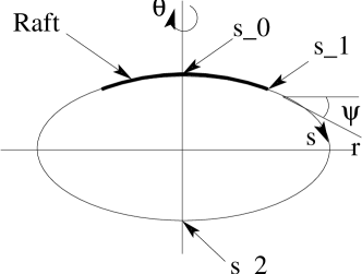
Figure 1: Parameterization of an axisymmetric vesicle with two phases in cylindrical coordinates.

The energy becomes:

$$F = 2\pi\left[{\int_{s_{0}}^{s_{1}}\mathcal{L}_{1}ds+\int_{s_{1}}^{s_{2}}\mathcal{L}_{2}ds+\sigma r(s_{1})}\right]$$ (4)

$$\mbox{with}\quad\mathcal{L}_{i}=\frac{\kappa_{i}}{2}\left({\frac{\sin(\psi)^{2}}{r}+\psi^{\prime 2}r+2\psi^{\prime}\sin(\psi)}\right)+\kappa_{G_{i}}\sin(\psi)\psi^{\prime}$$

$$-\Lambda_{i}\phi\left({\sin(\psi)+\psi^{\prime}r}\right)+\frac{\alpha_{i}}{2}\phi^{2}r+\frac{\beta_{i}}{2}\phi^{\prime 2}r+\Sigma^{\prime}_{i}r+\lambda^{\prime}_{i}\phi r$$

$$-\frac{P}{2}r^{2}\sin(\psi)+\gamma(r^{\prime}-\cos(\psi))$$

with the new parameters:

$$\Sigma_{i}^{\prime}=\Sigma_{i}+\frac{\alpha_{i}}{2}\phi_{eq_{i}}^{2}\quad\mbox{and}\quad\lambda_{i}^{\prime}=\lambda_{i}-\alpha_{i}\phi_{eq_{i}}.$$ (5)

Minimization with respect to small perturbations of the spatial coordinates ($r$ and $\psi$) and of the protein concentration $\phi$ leads to the E-L equations:

$$\psi^{\prime\prime} = \frac{\sin(\psi)\cos(\psi)}{r^{2}}-\frac{Pr}{2\kappa_{i}}\cos(\psi)-\frac{\psi^{\prime}}{r}\cos(\psi)+\frac{\Lambda_{i}}{\kappa_{i}}\phi^{\prime}+\frac{\gamma}{\kappa_{i}r}\sin(\psi),$$ (6a)

$$\gamma^{\prime} = \frac{\kappa_{i}}{2}\psi^{\prime 2}-\frac{\kappa}{2r^{2}}\sin(\psi)^{2}+\Sigma^{\prime}_{i}-Pr\sin(\psi)-\Lambda_{i}\phi\psi^{\prime}$$ (6b)

$$+\frac{\alpha_{i}}{2}\phi^{2}+\frac{\beta_{i}}{2}\phi^{\prime 2}+\lambda^{\prime}_{i}\phi,$$

$$\phi^{\prime\prime} = -\frac{\Lambda_{i}}{\beta_{i}r}(\sin(\psi)+\psi^{\prime}r)+\frac{\alpha_{i}}{\beta_{i}}\phi-\phi^{\prime}\frac{\cos(\psi)}{r}+\frac{\lambda^{\prime}_{i}}{\beta_{i}},$$ (6c)

$$r^{\prime} = \cos(\psi).$$ (6d)

The boundary conditions deduced from Eq.(4) at the junction (defined by $s_{1}$) between the two phases and the continuity of the radius $r$ give:

$$\kappa_{1}\psi^{\prime}(s_{1}-\epsilon)r(s_{1})+(\kappa_{1}+\kappa_{G_{1}})\sin(\psi(s_{1}-\epsilon))-\Lambda_{1}\phi(s_{1}-\epsilon)r(s_{1})$$ (7a)

$$-\kappa_{2}\psi^{\prime}(s_{1}+\epsilon)r(s_{1})-(\kappa_{2}+\kappa_{G_{2}})\sin(\psi(s_{1}+\epsilon))+\Lambda_{2}\phi(s_{1}+\epsilon)r(s_{1})=0,$$ (7c)

$$\gamma(s_{1}-\epsilon)-\gamma(s_{1}+\epsilon)+\sigma=0,$$

$$\beta_{1}\phi^{\prime}(s_{1}-\epsilon)r(s_{1})-\beta_{2}\phi^{\prime}(s_{1}+\epsilon)r(s_{1})=0.$$

The boundary conditions are deduced from the bounds in the variational process. The observation of a shape discontinuity at the boundary between the two phases webb03 suggests a solution which exhibits such a discontinuity of the slope at $s=s_{1}$. The angle $\psi$ between the surface and the radius axis is chosen discontinuous at the interface (see Fig.2). This allows a tilt of the surface at the boundary $C$. The simplest solution, strongly suggested by the experiment, is two spherical caps of radius $R_{1}$ and $R_{2}$, one for each phase with a constant concentration $\phi_{i}$ (see Fig.2, for clarity, the deformation of the raft is stronger than the real one in the initial state).

Figure 2: Parameterization of the vesicle near its initial state. The deformation is larger than the real one in the initial state.

The minimization shows that one must satisfy the following ”bulk” conditions for each phase in order to have this solution:

$$\lambda_{i}^{\prime}R_{i}=2\Lambda_{i}-\alpha_{i}R_{i}\phi_{i}\quad\mbox{so}\quad R_{i}\lambda_{i}=2\Lambda_{i}$$ (8a)

$$2\Sigma_{i}^{\prime}R_{i}^{2}-PR_{i}^{3}+2\Lambda_{i}\phi_{i}R_{i}-\alpha_{i}\phi_{i}^{2}R_{i}^{2}=0.$$ (8b)

The boundary conditions give two other relations:

$$\frac{2\kappa_{1}+\kappa_{G_{1}}}{R_{1}}-\Lambda_{1}\phi_{1}=\frac{2\kappa_{2}+\kappa_{G_{2}}}{R_{2}}-\Lambda_{2}\phi_{2},$$ (9a)

$$R_{2}\cos(\theta_{2})-R_{1}\cos(\theta_{1})=\frac{2\sigma}{PR_{1}\sin(\theta_{1})}.$$ (9b)

where $\theta_{1}$ and $\theta_{2}$ are the polar angles in each phase at the boundary (see Fig.2). Note that, for each phase, the couple of equations given by Eq.(8) derive the Lagrange parameters like $\lambda_{i}$ (equivalent to a chemical potential) and $\Sigma_{i}$ (the tension) which are quantities not easy to measure experimentally. On the contrary, Eq.(9) give geometrical informations. These informations with the other constraints such as the continuity of the radius and the ratio between area of both phases are enough to fix completely the values of $R_{1}$, $R_{2}$, $\theta_{1}$ and $\theta_{2}$. Both conditions have to be satisfied for all protein concentrations in order to ensure the existence of the initial homogeneous spherical caps, whether they are stable or not. If there is no protein, the conditions (8) reduce to $\lambda^{\prime}=0$ and $2\Sigma_{i}^{\prime}R_{0}^{2}=PR_{0}^{3}$, which is the classical Laplace equation for an interface with a surface tension. Contrary to the law of capillarity, where the surface tension is a physical parameter dependent on the chemical phases involved, the tension here is not a constant characteristic of the lipids of the vesicle. It is a stress (times a length) which varies with the pressure.

3.2 Linear perturbation analysis

Now, we examine the stability of this solution. Due to the geometry, it turns out that the spherical coordinate system is more appropriate here and make the calculations easier. A perturbation of the spherical cap (i) is described by: $R(\theta;\varphi)=R_{i}(1+u(\theta;\varphi))$ with $R_{i}$ the initial radius; in a similar way, a perturbation of the protein concentration is $\phi=\phi_{i}(1+v(\theta;\varphi))$ with $\phi_{i}$ the initial and homogeneous concentration of proteins on the surface. We assume that the line tension is not modified by the addition of proteins, at least linearly. One can expand the free energy Eq.(4) to second order in $u$ and $v$ in the phase $i$:

$$F_{i} = 2\pi\left[{\int_{s_{0_{i}}}^{s_{1_{i}}}\mathcal{L}_{i}(u,\nabla u,\Delta u,v,\nabla v)\sin\theta d\theta}\right]\quad\mbox{with}$$ (10)

$$\mathcal{L}_{i}=2\kappa_{i}\left({-\Delta u+\frac{1}{4}{\Delta u}^{2}+u\Delta u+\frac{{\nabla u}^{2}}{2}}\right)+\Sigma_{i}^{\prime}R_{i}^{2}\left({2u+u^{2}+\frac{{\nabla u}^{2}}{2}}\right)$$

$$-2\Lambda_{i}\phi_{i}R_{i}\left({u+v-\frac{\Delta u}{2}+\frac{{\nabla u}^{2}}{2}+uv-\frac{v\Delta u}{2}}\right)-\frac{PR_{i}^{3}}{3}(3u+3u^{2})$$

$$+\frac{\alpha_{i}}{2}(\phi_{i}R_{i})^{2}\left({2u+2v+u^{2}+4uv+v^{2}+\frac{{\nabla u}^{2}}{2}}\right)+\frac{\beta_{i}}{2}\phi_{i}^{2}(\nabla v)^{2}$$

$$+\lambda^{\prime}_{i}\phi_{i}R_{i}^{2}\left({2u+v+u^{2}+2uv+\frac{{\nabla u}^{2}}{2}}\right)$$

The total free energy is then a function of $u$ and $v$, which allows a variational approach to find the Euler-Lagrange’s equations (E-L equations) and the boundary conditions. The E-L equations give shapes which are extrema of the free energy. Two sets of equations are derived: one for the zeroth order in $u$ and $v$ and one for the first order, the energy being calculated up to the second order of the perturbation. The zero-order equations gives the same results as Eq.(9). The first order equations are:

$$\Lambda_{i}\phi_{i}R_{i}(2u+\Delta u)+\phi_{i}^{2}R_{i}^{2}\left({\alpha_{i}v-\frac{\beta_{i}}{R_{i}^{2}}\Delta v}\right)=0$$ (11a)

$$\left({-2\Lambda_{i}\phi_{i}R_{i}+2\alpha_{i}\phi_{i}^{2}R_{i}^{2}+2\lambda^{\prime}_{i}\phi_{i}R_{i}^{2}}\right)v+\Lambda_{i}\phi_{i}R_{i}\Delta v$$

$$+ \left({2\Sigma^{\prime}_{i}R_{i}^{2}+\alpha_{i}\phi_{i}^{2}R_{i}^{2}+2\lambda^{\prime}_{i}\phi_{i}R_{i}^{2}-2PR_{i}^{3}}\right)u$$

$$+ \left({2\kappa_{i}-\Sigma^{\prime}_{i}R_{i}^{2}+2\Lambda_{i}R_{i}\phi_{i}-\frac{\alpha_{i}}{2}\phi_{i}^{2}R_{i}^{2}-\lambda^{\prime}_{i}\phi_{i}R_{i}^{2}}\right)\Delta u+\kappa_{i}\Delta\Delta u=0$$

equivalent to

$$\Lambda_{i}\phi_{i}R_{i}(2v+\Delta v)+\left({\Lambda_{i}\phi_{i}R_{i}-\frac{PR_{i}^{3}}{2}}\right)(2u+\Delta u)+\kappa_{i}\Delta\left({2u+\Delta u}\right)=0$$ (11c)

This coupling imposes boundary conditions which must be treated at the zero-order and the first order. We have already studied the zero-order which gives relations (9). As usual for linear perturbation analysis, the boundary conditions for the perturbation are homogeneous: $u=\Delta u=v=0$ at the boundary between the two phases. Contrary to first intuition and usual procedures, although Eq.(11a) and (11c) are linear, we cannot use the Legendre polynomial basis, due to the specific boundary conditions in this problem. The convenient angular basis in this case turns out to be the spherical cap harmonics, following standard techniques in geophysics Haines85 (see Appendix A where we recall some mathematical useful relations). These spherical cap harmonics are Legendre functions $P_{x_{l}}(\cos\theta)$. The regular function at the pole of the cap is of the first kind and since we restrict on axisymmetric perturbations, these Legendre functions are simply hypergeometric function

$${{}_{2}}F_{1}\left({-x_{l},x_{l}+1,1,\frac{1-\cos\theta}{2}}\right).$$

Notice that $x_{l}$ is not an integer. In the case where it is, we recover the Legendre polynomial basis. We select the spherical cap harmonics which vanish at the boundary angle ($\theta=\theta_{1}$ or $\theta=\theta_{2}$, see Fig.2). This condition at the boundary gives a discrete infinite set of non-integer $x_{l}^{(i)}$ values for the phase ($i$). $l$ is an integer index used to order the allowed values $x_{l}^{(i)}$ by increasing values. It is also the number of zero of the function $P_{x_{l}^{(i)}}$ on the cap. These harmonics have the properties to be an orthogonal basis and to be eigenfunctions of the Legendre equation with eigenvalues: $x_{l}^{(i)}(x_{l}^{(i)}+1)$. We define $u(\theta)=\Sigma_{l}u_{l}P_{x_{l}}(\cos\theta)$ and $v(\theta)=\Sigma_{l}v_{l}P_{x_{l}}(\cos\theta)$. From the first E-L equation (11a), one can deduce the amplitude $v_{i,l}$ the protein concentration from $u_{i,l}$ in the phase ($i$):

$$v_{i,l}=\frac{\Lambda_{i}\left[{x_{l}^{(i)}(x_{l}^{(i)}+1)-2}\right]}{\phi_{i}R_{i}\left[{\alpha_{i}+\beta_{i}(x_{l}^{(i)}+1)x_{l}^{(i)}/R_{i}^{2}}\right]}u_{i,l}.$$ (12)

We introduce $q^{2}=x_{l}^{(i)}(x_{l}^{(i)}+1)/R_{i}^{2}$, which is similar to the spatial period of the perturbation. Then, from the second E-L equation (11) and after elimination using Eq.(12), we derive

$$\Lambda_{i}^{2}(q^{2}-2/R_{i}^{2})=\left({\Sigma_{i}^{\prime}-\frac{\alpha_{i}}{2}\phi_{i}^{2}+\kappa_{i}q^{2}}\right)(\alpha_{i}+\beta_{i}q^{2}).$$ (13)

Our result can be compared to previous analysis made in two different asymptotic limits in the homogeneous case. In these cases, the cap is a complete sphere and $x_{l}$ is an integer. First, for $\beta=0$, we recover the result of Mori93 for an homogeneous vesicle without diffusion. Second, when $R_{i}$ goes to infinity, we recover the result for an homogeneous flat membrane Leibler86 .

Notice that, in Eq.(13), the protein concentration has a similar significance as a negative surface tension: one can make the change of variable $\Sigma_{i}^{\prime\prime}=\Sigma_{i}^{\prime}-\alpha_{i}\phi^{2}_{i}/2=\Sigma_{i}+\alpha_{i}(\phi_{eq_{i}}^{2}-\phi^{2}_{i})/2$. The principal effect of the proteins is to decrease the surface tension which is an obvious sign of instability.

4 Discussion

We will use the protein concentration $\phi_{i}$ as our control parameter. Eq.(13) gives for each mode $x_{l}^{(i)}$ a threshold concentration $\Phi_{i}$ such that for $\phi_{i}\leq\Phi_{i}$ the initial state is stable and for $\phi_{i}\geq\Phi_{i}$, one of the two phases is unstable, leading to a complete instability. The threshold concentration $\Phi_{i}$ strongly depends on the physical properties of each phase. Then, the two parts of the initial system have no reason to be unstable simultaneously. The deformation of the other phase (not unstable to linear order) will be induced by the non-linear effects not included in this analysis.

Since the thermal energy $kT$ is the only external energy and the typical length of the phase (i) is $R_{i}$, one can introduce dimensionless parameters: $\tilde{q}=x_{l}(x_{l}+1)$, ${\kappa}_{i}=\kappa_{i}/kT$, $\tilde{\Sigma}_{i}^{\prime}=\Sigma_{i}R_{i}^{2}/kT$, $\tilde{\Lambda}_{i}=\Lambda_{i}/(kTR_{i})$, $\tilde{\alpha}_{i}=\alpha_{i}/(R_{i}^{2}kT)$ and $\tilde{\beta}_{i}=\beta_{i}/(R_{i}^{2}L_{c}^{2}kT)$ with $L_{c}$ a characteristic length for the gradient of protein concentration. Then, the protein concentration is replaced by $R_{i}^{4}\phi_{i}^{2}$ which is proportional to the square of the number of proteins in the phase (i).

Rewriting the threshold (13), we find for the threshold concentration, in dimensionless parameters:

$$R_{i}^{4}\Phi_{i}^{2}=\frac{2}{\tilde{\alpha}_{i}}\left({\tilde{\Sigma}_{i}^{\prime}+\tilde{\kappa}_{i}\tilde{q}^{2}-\frac{\tilde{\Lambda}_{i}^{2}(\tilde{q}^{2}-2)}{\tilde{\alpha_{i}}+\tilde{\beta}_{i}(L_{c}/R_{i})^{2}\tilde{q}^{2}}}\right).$$ (14)

From Eq.(14), the search of the smallest threshold concentration gives two different regimes depending on the value of the dimensionless constant:

$$c=\frac{\tilde{\Lambda_{i}}^{2}\left({\tilde{\alpha_{i}}+2\tilde{\beta_{i}}\frac{L_{c}^{2}}{R_{i}^{2}}}\right)}{\tilde{\kappa_{i}}\tilde{\alpha_{i}}^{2}}=\frac{\Lambda_{i}^{2}(\alpha_{i}+2\beta_{i}/R_{i}^{2})}{\kappa_{i}\alpha_{i}^{2}}.$$ (15)

This constant describes the strength of the coupling of the protein with the membrane ($\Lambda_{i}$) to the resistance of the membrane ($\kappa_{i}$) and to the absorption power ($\alpha_{i}$).

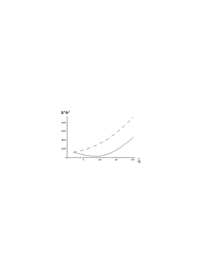
Figure 3: Threshold concentration versus the reduced mode$\tilde{q}$ for two different values of (14) are taken as $\tilde{\alpha}_{i}=1$, $\tilde{\kappa}_{i}=1$, $\tilde{\Sigma}_{i}^{\prime}=60$, $\tilde{\beta}_{i}(L_{c}/R_{i})^{2}=0.01$. The solid line is the case of large tilt due to each protein: $\tilde{\Lambda}_{i}=1.7$. The dashed curve is the case of a small tilt: $\tilde{\Lambda}_{i}=0.01$.

In the weak interaction regime ($c\leq 1$), the protein concentration is an increasing function of $\tilde{q}$ (see fig. 3). So, the threshold is obtained for the smallest possible $x_{l}$: $x_{0}$. The direction of the deformation (inside or outside the initial cap) would be deduced from a third order calculation or from a numerical simulation. According to the definition of $\Sigma_{i}^{\prime}$ (Eq.(5)), the concentration required to destabilize the membrane is found bigger than the equilibrium concentration. But in this case, one expects that this threshold $\Phi_{i}$ is difficult or impossible to reach since it requests the absorption of a concentration of proteins larger than $\phi_{eq_{i}}$: probably, the excess of proteins would prefer to dissolve in the surrounding water then forming aggregates. So, the weak regime of instability is not observable experimentally, our basic state made of two spherical caps is stable and proteins are stocked only.

In the strong interaction regime, the limiting concentration shows a minimum not necessary for the smallest $x_{l}$ (see fig.3). This has two consequences. First, the limiting concentration is less than the equilibrium concentration and it is easier to induce the instability. Second, the first unstable mode could be modified: $\tilde{q}\approx 10$ for the chosen numerical values. So, we have something more complex than the simple oblate/prolate ($x_{0}$) deformation. This regime is observable and probably corresponds to the observed shape instability. In any case, our basic state cannot be seen in the experiment except as a transient.

The existence of these two regimes, depending on the nature of the proteins, allows two possible and distinct scenarios for the cell: there is no doubt that this property is useful and probably used for biological purpose. The main difficulty of this study is the quantitative determination of the parameters since experimental values are not available even for this minimal model. Let us estimate $c$. The curvature of the membrane is of order $1/R_{i}$, its surface is close to $R_{i}^{2}$. $\kappa$ is of order $10kT$ for an unstretched vesicle, so $\tilde{\kappa}\approx 10$. $\alpha$, the cost of energy needed to increase the concentration of proteins, can be deduced from the energy required to remove a protein from the surface which is is about $100kT$. It changes the concentration of proteins of $1/R_{i}^{2}$ so $100kT=\alpha_{i}/R_{i}^{2}$ and $\tilde{\alpha}\approx 100$. $\beta$ is deduced from $L_{c}$ which should be a small fraction of the radius of the sphere. We will take hereafter $L_{c}\approx R_{i}/10$. The proteins are moving at the surface of the membrane due to the Brownian motion. So the energy to move one protein by the length $L_{c}$ is about $kT$. Then, $\beta_{i}=kTL_{c}^{2}R_{i}^{2}$ and $\tilde{\beta_{i}}\approx 1$. The value of $\Lambda_{i}$ is more difficult to determine. $\Lambda_{i}$ is the coupling constant between the membrane and the proteins. This is expressed by the spontaneous curvature radius $R_{P}$. If $R_{P}$ is small, the coupling effect is strong and, on the opposite, if $R_{P}$ is large, $\Lambda_{i}$ is small, which suggests that $\Lambda_{i}$ is proportional to $1/R_{P}$. But $\Lambda_{i}$ is an energy multiplied by a length. Then, a good order of magnitude for $\Lambda_{i}$ is $kTR_{i}^{2}/R_{P}$, so $\tilde{\Lambda_{i}}=R_{i}/R_{P}$. Finally, we get $c\approx R_{P}/R_{i}$. If $R_{P}$ is smaller than $R_{i}$, the system is in the strong coupling regime and in the other case, the interaction between membrane and proteins is weak. When the two phases have approximately the same physical constants webb03 , the instability occurs first in the largest phase, as shown by Eq.(14) in the previous conditions. Nevertheless, the ejection of one part of the membrane requires a complete nonlinear dynamical treatment which will be derived from this energy formulation.

5 Conclusions

We have proposed a model of instability for an inhomogeneous vesicle which absorbs proteins. This instability is at the origin of a separation into two vesicles, one for each phase as seen experimentally. Our model rests on a ”bulk” effect and assumes that the proteins are distributed everywhere on the membrane contrary to the ”line tension ”model which assumes a high concentration of the proteins at the raft boundary. To validate (or invalidate) our model, an experimental test could be the use of phosphorescent proteins with the same properties. It would be a way to follow the place where the proteins prefer to diffuse and stay on the membrane. Although we ignore the feasibility of such an experiment, it would provide a very useful information.

We thank G. Staneva, M. Angelova and K. Koumanov for communicating their results prior to publication. We acknowledge enlightening discussions with J.B. Fournier.

Appendix A Spherical cap harmonics

The spherical cap harmonics are eigenvalues of the Laplace’s equation in spherical coordinates. The Laplace’s problem can then be rewritten as a Legendre’s equation. The general solution is:

$$U^{m}_{n}=f(\phi)L^{m}_{x_{l}}(\cos\theta)$$

with $\theta$ the colatitude, $\phi$ the longitude and $L^{m}_{x_{l}}$ an associated Legendre function. The eigenvalues associated to this solution are $m^{2}$ and $-x_{l}(x_{l}+1)$. So the solutions are symmetric with respect to $x_{l}=-1/2$. So we can restrict to $x_{l}\geq-1/2$ in all cases.

Generally speaking, $m$ and $x_{l}$ can be integer, real or even complex and are determined by the boundary conditions. For a sphere, the solution must be periodic in the $\phi$ angle. This implies $m$ real. In the particular case of an axisymmetric solution, which is the case in this paper, $m=0$.

The boundary condition on $\theta$ for $\theta=0$ is a condition of regularity:

$$\frac{\partial U^{0}_{x_{l}}}{\partial\theta}=0\quad\mbox{for}\quad m=0$$ (16)

$$U^{m}_{x_{l}}=0\quad\mbox{for}\quad m\neq 0$$ (17)

It is satisfied by the Legendre functions of the first kind and excludes those of the second kind. Notice that this condition is required both for a complete sphere and for a spherical cap.

In the case of the sphere, the boundary condition $\theta=\pi$ is similar to Eq.(16). The values of $x_{l}$ are then integer and the solutions are the classical associated Legendre polynomials.

For a spherical cap whose ends are given by $\theta=\pm\theta_{0}$, the boundary conditions at $\theta_{0}$ are given by standard physical requirements. These boundary conditions can be satisfied by using two kinds of solutions such that either:

$$\frac{\partial U^{m}_{x_{l}}}{\partial\theta}=0\quad\mbox{for}\quad\theta=\pm\theta_{0}$$ (18)

or:

$$U^{m}_{x_{l}}=0\quad\mbox{for}\quad\theta=\pm\theta_{0}$$ (19)

These conditions are satisfied by Legendre functions $P^{m}_{x_{l}}(\cos\theta)$ with $x_{l}$ not necessary integer. No function can satisfy simultaneously the conditions (18) and (19) and there is two sets of $x_{l}$ which depend on the $m$ value. We call $y_{l}(m)$ the values of $x_{l}$ such as (18) is satisfied and $z_{l}(m)$ the values of $x_{l}$ such as (19) is satisfied.

Functions in one set are orthogonal to each other but are not orthogonal to those of the other set. It is easy to show that:

$$\int_{0}^{\theta_{0}}{P^{m}_{y_{l_{1}}(m)}(\cos\theta)P^{m}_{y_{l_{2}}(m)}(\cos\theta)\sin\theta d\theta}=0\quad\mbox{for}\quad l_{1}\neq l_{2}$$

$$\int_{0}^{\theta_{0}}{P^{m}_{z_{l_{1}}(m)}(\cos\theta)P^{m}_{z_{l_{2}}(m)}(\cos\theta)\sin\theta d\theta}=0\quad\mbox{for}\quad l_{1}\neq l_{2}$$

$$\int_{0}^{\theta_{0}}{P^{m}_{y_{l_{1}}(m)}(\cos\theta)P^{m}_{z_{l_{2}}(m)}(\cos\theta)\sin\theta d\theta}=$$

$$\quad\quad\quad-\frac{\sin\theta_{0}P^{m}_{y_{l_{1}}(m)}(\cos\theta)\{[P^{m}_{z_{l_{2}}(m)}(\cos\theta)]/d\theta\}}{(y_{l_{1}}-z_{l_{2}})(y_{l_{1}}+z_{l_{2}}+1)}$$

If the physics requires the boundary condition (18) or (19), the set of solutions $y_{l}$ or $z_{l}$ is enough to form a basis of solution of the problem. In the other case, one have to combine both of them and the resolution of the complete problem becomes more harder. In the case of this paper, we focus on the case of axisymmetric solutions $(m=0)$. The boundary conditions are given by 19, so the good set of parameters are the $y_{l}(0)$. The table 1 presents the first values of $y_{l}$, calculated for two angles $\theta_{0}$ ($\pi/6$ and $5\pi/6$), chosen as example. The figure 4 shows the three first $P_{s_{l}}$ for $\theta_{0}=\pi/6$. The figure 5 shows the three first $P_{x_{l}}$ for $\theta_{0}=5\pi/6$. The figure 6 shows the deformation of the spherical cap in the case of a perturbation by the three first $P_{x_{l}}$ for $\theta_{0}=\pi/6$.

$l$	0	1	2	3	4	5	6
$\theta_{0}=\pi/6$	4.08	10.04	16.03	22.02	28.01	34.01	40.01
$\theta_{0}=5\pi/6$	0.35	1.57	2.78	3.98	5.19	6.39	7.59

Table 1: Values of $y_{l}$ for $m=0$ for the $7$ first values of $l$.

Figure 4: Legendre functions $P_{y_{l}}$ versus the angle $\theta$ for $\theta_{0}=\pi/6$ and for $l=0$ (solid curve), $l=1$ (large dashing) and $l=2$ (small dashing)

Figure 5: Legendre functions $P_{y_{l}}$ versus the angle $\theta$ for $\theta_{0}=5\pi/6$ and for $l=0$ (solid curve), $l=1$ (large dashing) and $l=2$ (small dashing)

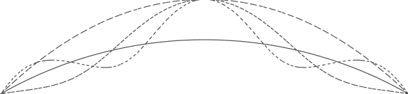
Figure 6: Deformations of a spherical cap of radius 1 and half-angle $\pi/6$. The deformations are dues to Legendre functions $P_{y_{l}}$. For clarity, the maximum amplitude of the deformation is fixed to 0.1. This value is too large in principle for the linear analysis. The solid curve is the initial state. The largest dashing is the case $l=0$. The intermediate dashing is the case $l=1$. The smallest dashing is the case $l=2$.

References

- (1) S. J. Singer and G. L. Nicolson, Science 175, 720 (1972)
- (2) D. A. Brown and J. Rose, Cell 68, 533 (1992)
- (3) K. Simons and E. Ikonen, Nature 387, 569 (1997) ; D. A. Brown and E. London, J. Biol. Chem. 275 (23), 17221 (2000) ; G. van Meer, Science 296, 855 (2002)
- (4) T.-Y. Wang and J. R. Silvius, Biophys. J. 84 (1), 367 (2003)
- (5) C. Dietrich et al., Biophys. J. 82 (1), 274 (2002)
- (6) W. L. Smith and A. H. Merrill, J. Biol. Chem. 277 (29), 25841 (2002)
- (7) G. Van Meer and Q. Lisman, J. Biol. Chem. 277 (29), 25855 (2002)
- (8) C. Dietrich et al. , Biophys. J. 80 (3), 1417 (2001)
- (9) S. L. Veatch and S. L. Keller, Phys. Rev. Lett. 89 (26), 268101 (2002)
- (10) G. Staneva, M. Angelova and K. Koumanov to be published in Journal of Chemisty and Physics of Lipids
- (11) T. Baumgart,S. T. Hess and W.W.Webb, Nature 425 ,821-825 (2003)
- (12) C.-M. Chen, P.G. Higgs, F.C. MacKintosh, Phys. Rev. Lett. 79, 1579-1582 (1997)
- (13) P. B. Canham, J. Theor. Biol 26, 61 (1970)
- (14) W. Helfrich, Z. Naturforsch., Teil C 28, 693 (1973)
- (15) L. Miao, B. Fourcade, M. Rao, M. Wortis, Phys. Rev. A 43 (12), 6843-6854 (1991)
- (16) U. Seifert, K. Berndl, R. Lipowsky, Phys. Rev. A 44 (2), 1182-1202 (1991)
- (17) M. Jaric, U. Seifert, W. Wintz, M. Wortis, Phys. Rev. E 52 (6), 6623-6634 (1995)
- (18) F. Jülicher and R. Lipowsky, Phys. Rev. E 53 (3), 2670 (1996)
- (19) H.-G. Döbereiner, E. Evans, M. Kraus, U. Seifert, M. Wortis, Phys. Rev. E 55 (4), 4458-4474 (1997)
- (20) U. Seifert, Adv. in Phys. 46 (1), 13-137 (1997)
- (21) S. Leibler, J. physique 47, 507-516 (1986)
- (22) U. Seifert, Phys. Rev. Lett. 70 (9), 1335-1338 (1993)
- (23) J.-B. Fournier, A. Adjari, L. Peliti, Phys. Rev. Lett. 86 (21), 4970-4973 (2001)
- (24) F. Daumas, N. Destainville, C. Millot, A. Lopez, D. Dean, L. Salomé, Biophys. J. 84 (1), 356-366 (2003)
- (25) T. Bickel, C. Marques, Phys. Rev. E 62 (1), 1124-1127 (2000)
- (26) F. Brochard, P. G. De Gennes and O. Sandre, Physica A 278 (1-2), 32 (2000)
-
(27)
G.V. Haines, J. Geophys. Rev. 90, 2583 (1985)
W.R. Smythe, Static and Dynamic Electricity, 2nd ed., McGraw-Hill, New-York, 1950
A.E. Love, A treatise on the mathematical theory of elasticity, Dover, New-York, 1944 - (28) S. Mori and M. Wadati, J. Phys. Soc. Jap. 62 (10), 3557 (1993) label