Nonlinear Theory and Its Applications Michael SmallNon-member* Pengliang ShiNon-member* Chi Kong TseNon-member* [*]The authors are with the Department of Electronic and Information Engineering of the Hong Kong Polytechnic University 11 11 200311

Plausible models for propagation of the SARS virus

Using daily infection data for Hong Kong we explore the validity of a variety of models of disease propagation when applied to the SARS epidemic. Surrogate data methods show that simple random models are insufficient and that the standard epidemic susceptible-infected-removed model does not fully account for the underlying variability in the observed data. As an alternative, we consider a more complex small world network model and show that such a structure can be applied to reliably produce simulations quantitative similar to the true data. The small world network model not only captures the apparently random fluctuation in the reported data, but can also reproduces mini-outbreaks such as those caused by so-called “super-spreaders” and in the Hong Kong housing estate Amoy Gardens.

1 SARS in the SAR

The redundantly named Severe Acute Respiratory Syndrome (SARS) [1] appeared in the Guangdong province of China in November 2002 and spread to the Hong Kong SAR. From Hong Kong, the virus spread throughout the world: largely due to the airline (small world) network hub in Hong Kong. The economic and social effects of the SARS virus have been subject of much attention in the popular media [2] and have been widely reported. Less well reported, but no less unusual is the effect this disease had on academic activities, including the cancellation of the 2003 International Symposium on Nonlinear Theory and its Applications.

In this report we analyse the SARS daily infection data for Hong Kong and test the validity of three distinct types of models: (i) stochastic models generated from surrogate data; (ii) standard susceptible-infected-removed (SIR) models; and (iii) small world network models. We find that the small world network models are the only models capable of reproducing the quantitative behaviour of the SARS epidemic in Hong Kong. Moreover, these models also exhibit many features characteristic of this epidemic: a small fraction of individuals show a very great propensity to infect others (the “super-spreaders”); and, propagation of the virus within certain physical locations led to a large number of infections (the outbreaks in Prince of Wales Hospital and Amoy Gardens Housing Estate).

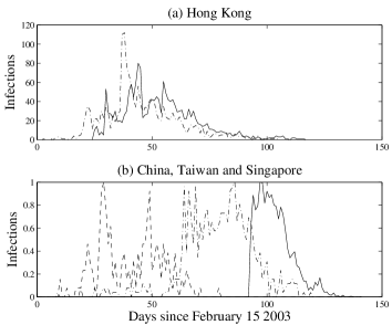
Figure 1: Daily reported SARS infections. The top plot shows the daily number of SARS infections in Hong Kong. The lower plot are the daily number of infections in Taiwan (dot-dashed), Singapore (dashed), and the Chinese mainland (solid). For the purpose of comparison, the numbers on the lower plot are normalised by the maximum daily infection tally. The maximum daily infection tally for Taiwan, Singapore and China was 26, 13 and 203. The data for Taiwan and Singapore has been revised based on case information after the epidemic, this has not been possible for the China data.

Figure 1 shows the daily infection rate for SARS in Hong Kong between 15 February 2003 and 15 June 2003. Compared to the data for other territories (lower panel of Fig. 1), the data for Hong Kong appears to be more complete (compared to Taiwan), more accurate (compared to the Chinese mainland) and over a longer time period (compared to Singapore). The data for Hong Kong is shown as two time series, the original daily number of infections, as recorded by the Hong Kong Department of Health, and revised figures released after a more detailed analysis of the true infection path [3]. The revised data offers a more accurate picture of the true daily number of infections, but this data uses information not available at the time of the outbreak and we therefore do not analyse that data in this report.

For the current analysis, let $x_{t}$ denote the number of infections reported in the Hong Kong media (based on statistics published by the Hong Kong department of Health) for day $t$ and we start with $x_{0}=0$. Hence $t$ is the number of days since 11 March 2003 (March 12 is the first day of recorded infections in Hong Kong, infections prior to this date were only identified in the revised data). For notational convenience we denote the entire time series as $\{x_{t}\}_{t}=\{x_{t}\}_{t=0}^{N}=(x_{0},x_{1},x_{2},\ldots,x_{N})$.

The remainder of this paper describes the analysis of the original data in Fig. 1(a) with three different model structures. In the next section we describe the application of surrogate data techniques to test the Hong Kong SARS time series against the hypothesis that inter-day variability in the reported incidence of SARS is random. In Section 3 we assess the accuracy of the SIR model and in Section 4 we describe the small world network model.

2 Random variability

The simplest model of disease propagation is that of a random walk such that $x_{0}=x_{N}=0$ and $x_{t}\geq 0$ for $t=0,\ldots,N$. The duration of the disease, $N$, is essentially a random variable. The inter-day variation is random and, according to the Central Limit Theorem, the disease will eventually die out.

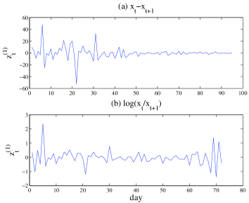
Figure 2: Inter-day variability. Variability between daily values plotted as the difference $x_{t}-x_{t+1}$ (top plot), or log ratio $\log\frac{x_{t}}{x_{t+1}}$ (lower plot).

Our first task is to transform the data in Fig. 1 to have zero mean and be approximately independent and identically distributed (i.i.d.). We do this by taking the difference of successive values

$$z^{(1)}_{t}=x_{t}-x_{t+1}$$

or taking the log-ratio of successive values

$$z^{(2)}_{t}=\log{\frac{x_{t}}{x_{t+1}}}.$$

Both $\{z^{(1)}_{t}\}_{t}$ and $\{z^{(1)}_{t}\}_{t}$ are depicted in Fig. 2. We note that because there is an underlying pattern in $\{|x_{t}|\}_{t}$ we expect that $\{z^{(2)}_{t}\}_{t}$ will offer a time series closer to i.i.d than $\{z^{(1)}_{t}\}_{t}$.

We now apply the method of surrogate data [4, 5] to determine whether the transformed data in Fig. 2 is statistically distinct from i.i.d. noise. Note that this is equivalent to testing whether the raw time series $\{|x_{t}|\}_{t}$ is a random walk.

To test for i.i.d. noise the method of surrogate data specifies that one should generate an ensemble of surrogate data sets. Each surrogate data set is a realisation of an i.i.d. process, but is otherwise “like” the original data. From this ensemble of surrogates one estimates some statistical quantity and compares this distribution of statistic values to the statistic value for the true data. If the true data has a statistical value typical of the surrogates then the underlying hypothesis (in this case, that the data is i.i.d.) may not be rejected. If the data is atypical of the surrogate distribution then the hypothesis may be rejected.

To generate suitable surrogates, we wish to destroy temporal correlation but preserve the data’s probability density function. The simplest way to do this is by randomly shuffling either without [4] or with [6] replacement. The choice of suitable test statistic is also important [7]. In our past experience we have advocated correlation dimension [7] or other dynamic invariants [5]. However, for such extremely short time series this is inappropriate. We attempted to use nonlinear complexity [8] as a measure, but found that this index exhibited extremely low sensitivity. We instead settle on the normalised covariance between $x_{t}$ and $x_{t+1}$

$$\frac{<x_{t}x_{t+1}>}{<x_{t}^{2}>}.$$

One further advantage of this simple measure is that it is sensitive to linear dependence: exactly the property we wish to detect. Unfortunately, this also means that testing more complex linear surrogate hypotheses will not be possible. Hence, as suggested by Takens [9] we prefer to test the model residuals against the i.i.d. hypothesis.

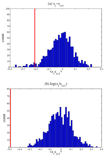
Figure 3: Surrogate calculations. The normalised covariance of $x_{t}$ and $x_{t+1}$, is plotted for the two time series in Fig. 2, along with $1000$ shuffled surrogates. In both cases the hypothesis that the data in Fig. 2 is independent and identically distributed noise is soundly rejected ($p>0.95$).

The results of Fig. 3 clearly indicate that the data of Fig. 2 is not consistent with an i.i.d. noise source. Therefore the original data (Fig. 1) may not be modelled as a simple random walk.

It would be logical to continue this analysis with more sophisticated surrogate algorithms [4, 10]. However, for this short time series results of more sophisticated algorithms are not conclusive. Furthermore, as we have already noted, it would not be possible to apply the covariance as a discriminating statistic in these cases, as the surrogate algorithms explicitly preserve autocorrelation. Instead, in the following section we consider a simple deterministic model of disease propagation.

3 SIR models

The standard Susceptible-Infected-Removed (SIR) model of disease propagation has a long history and is considered in detail in any standard text on mathematical biology [11]. In difference equation form, the relationship between the three populations at time $t$ may be expressed as

$$\left(\begin{array}[]{c}S_{t+1}\\ I_{t+1}\\ R_{t+1}\end{array}\right) = \left(\begin{array}[]{c}S_{t}(1-rI_{t})\\ (rS_{t}+(1-a))I_{t}\\ R_{t}+aI_{t}\end{array}\right)$$ (7)

where $S_{t}$, $I_{t}$, $R_{t}$ are the number (or proportion) of individual that are susceptible to infection, infected and “removed” respectively. Not that, by removed, we mean individuals that have been infected but are no longer infectious or susceptible. Such individuals may be cured (and immune), quarantined, or dead. The parameters $r$ and $a$ are the infection rate and the removal rate respectively.

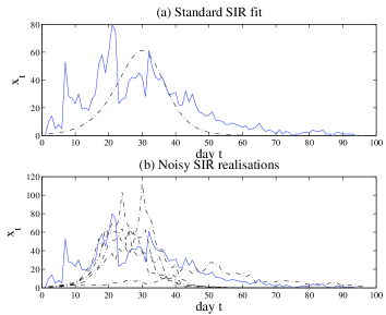
Figure 4: SIR models of SARS. The top plot shows the daily number of SARS infections in Hong Kong and the best fit SIR model. The lower shows five simulations from this model with multiplicative noise (described in the text) on the daily number of new infections

Using the SIR data we obtain a maximum likelihood estimate (i.e. minimum least squares fit) of the parameters $a$ and $r$ for the Hong Kong SARS time series. The time series in Fig. 1 is the number of new infections reported each day. This corresponds to the term $rS_{t}I_{t}$ in Eqn. (7). The numerical fitting procedure often estimates (incorrectly) a monotonically increasing of decreasing function. To prevent these solutions, we add leading and trailing zeros to the data prior to fitting. This helps to ensure that the optimal model exhibits a single extremum — not at either endpoint. An alternative to fitting $rS_{t}I_{t}$ to the observed data would be to also consider the daily fatality and recovery data for Hong Kong as an approximation for $\Delta R_{t}$. One could then fit $\Delta I_{t}$ and $\Delta R_{t}$ directly from the observed data.

In Fig. 4 (a) we see the time course of the best model (Eqn. (7)) fitted from this data. Clearly, this deterministic model does not capture the random variation observed in the data.

One way of considering this random variation is that the SIR model provides an estimate of the rate of infection (i.e. $I_{t+1}=(rS_{t}+(1-a))I_{t}$), but that this estimate is subject to random fluctuations. It may be better therefore to perturb the number of new infections by some unknown quantity $\epsilon_{t}$. The modified, stochastic SIR equations then read

$$\left(\begin{array}[]{c}S_{t+1}\\ I_{t+1}\\ R_{t+1}\end{array}\right) = \left(\begin{array}[]{c}S_{t}(1-rI_{t})-\epsilon_{t}\\ (rS_{t}+(1-a))I_{t}+\epsilon_{t}\\ R_{t}+aI_{t}\end{array}\right).$$ (14)

A similar random term could be added to the rate of removal, however we do not consider this problem here. Moreover, arbitrarily complex noise inputs could be devised that would eventually reproduce features of the observed data. Our concern is only whether these features can be observed from the SIR model, or immediate generalisations of this model.

We found that simulations with $\epsilon_{t}\sim N(0,\sigma^{2})$ for a constant $\sigma^{2}$ did not produce realistic simulations. The problem is that the magnitude of the random fluctuation should be proportional to the number of infected individuals. Few infected individuals are unlikely to have a great variation in effect, but many such individuals will. In Fig. 4 (b) we show five simulations with the noise term $\epsilon_{t}\sim N(0,(I_{t}\sigma)^{2})$. To ensure that the model is physically realistic (i.e. non-negative populations) we also restrict $\epsilon_{t}>-(rS_{t}+(1-a))I_{t}$. We found that $\sigma\approx 0.25$ gave quantitatively reasonable results and this is the value employed in Fig. 4.

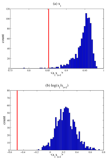
Figure 5: Surrogate calculations for stochastic SIR data. The normalised covariance of $x_{t}$ and $x_{t+1}$, is plotted for the data along with $1000$ independent model simulations (this is a similar calculation to that depicted in Fig. 3 (b)). The statistics in panel (a) and (b) differ. In panel (a) the normalise covariance of the data is estimated, in panel (b) the normalised covariance of the log-ratio of the data is computed. In both cases the hypothesis that the SIR model is a good model is soundly rejected ($p\geq 0.95$).

To quantitatively evaluate the effectiveness of the SIR type models (Eqn. (14)) we apply a variant on the method of surrogate data [7]. However, instead of generating constrained realisations consistent with the null hypothesis, we generate multiple realisations of the model and compare these realisations to the data [9]. For the model described by Eqn. (14) we generate $1000$ simulations and for each simulation compute $<x_{t}x_{t+1}>$ and $<z_{t}z_{t+1}>$ where $z_{t}=\log\frac{x_{t}}{x_{t+1}}$. That is, we use two distinct test statistics. Results for both statistics are plotted in Fig. 5 show a clear distinction between data and surrogates. Since this model is the optimal fit to the data and the distribution of covariance estimates do not vary greatly with change in model parameters, we therefore conclude that models of the form Eqn. (14) are not adequate to describe the underlying dynamics.

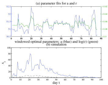
Figure 6: Variable parameters ($a$,$r$). The top plot shows the best fit estimates of the parameters $a$ and $r$ where the parameters are fitted to a window of $10$ successive data. The lower plot shows a deterministic prediction using these variable values.

One widely accepted reason for the failure of the SIR models is that the parameters $a$ and $r$ do not remain constant during the time course of an epidemic. Particularly when a disease is previously unknown and public health practice changes significantly in response to the spread of the disease. This is certainly consistent with the situation for SARS in Hong Kong. We therefore modify the SIR model of Eqn. (7) by estimating the temporal dependence of $a$ and $r$. We apply a sliding window of width 10 days and re-estimate $a$ and $r$ for every day. Figure 6 depicts the results of this computation. The values $a_{t}$ and $r_{t}$ are based on the best fit estimate of Eqn. (7) to the data $(x_{t},x_{t+1},x_{t+2},\ldots,x_{t+10})$.

While the simulations in Fig. 6 (b) does have the correct shape, if not the correct magnitude, the values of $a$ and $r$ depicted in Fig. 6 (a) illustrate the problem with this approach. The parameter values are sensitively dependent on the observed data and do not reflect reality. In a separate publication we modify this approach by considering longer windows and have shown the utility of the ratio $r/a$ for estimating the effectiveness of various governmental control strategies [13]. A combination of the random fluctuations approach of Eqn. (14) and the variability in $a$ and $r$ may produce more realistic simulations. However, we feel that this would represent a significant over-parameterisation of this modelling problem.

For the current investigation we conclude that a general SIR model is unable to capture the underlying dynamics of the system. More exotic SIR inspired models, or more contrived noise inputs, may be able to reproduce the observed behaviour. Indeed, we expect this should be the case when the system becomes complex enough. But this is beyond the focus of the current communication and is in general a less interesting problem. In the following section we consider a computationally more extensive model that is inspired by the physical situation and provides a more realistic alternative.

4 Small world networks

The final model structure we examine is computationally more complex, but also more realistic. In contrast to potentially exotic modified SIR models, the model we introduce here is inspired by our understanding of the physical situation. Small world networks (SWN) [14] have recently become immensely popular and received significant attention in a wide variety of fields [15]. One system which has provided evidence of small world structure is the network of social interaction between individuals (the so-called “six degrees of separation”). It is therefore natural to consider propagation of disease epidemics between nodes of a SWN.

In the following SWN we suppose that each node is either susceptible to disease (S), infected (I) or removed (R). However, unlike the standard SIR structure, nodes of the SWN can only infect those that they are acquainted with. We arrange the nodes in a rectangular grid (for Hong Kong, we use a square with side length $2700$). On a given day, each node can infect $n_{1}$ of its four immediate neighbours (horizontally and vertically) with constant probability $p_{1}$. Each node also has a random number of long range acquaintances. The number of long range acquaintances follows an exponential distribution with an expected value of $n_{2}$ and the acquaintances are chosen at random but fixed for each node. On each day, each of the long range acquaintances may be infected with some constant probability $p_{2}$. Finally, on each day, every infected node has probability $r_{1}$ of becoming removed. As with the SIR model, the only possible transitions are $S\rightarrow I\rightarrow R$.

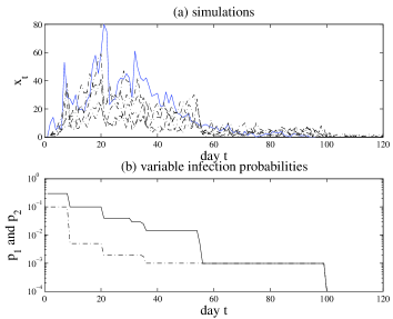
Figure 7: Variable parameters ($p_{1}$,$p_{2}$). The top plot is the Hong Kong SARS data together with five simulations of small world network model with the variables $p_{1}$ and $p_{2}$ changing with time (presumably in response to changing public health practice). The bottom plot shows the variation in the parameters $p_{1}$ and $p_{2}$ used in the top plot. These values were selected using an ad hoc process.

For our first simulations we simplify this structure by setting $r_{1}=0$. To avoid eventual complete contamination we vary (i.e. decrease) $p_{1}$ and $p_{2}$ with time according to the scheme in Fig. 7 (b). The values depicted in Fig. 7 are selected only because they yield a model with has a realistic behaviour. Figure 7 (a) compares five random realisations of $\Delta S_{t}$ to the observed data. We see that the quantitative features are reproduced nicely.

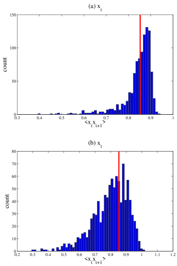
Figure 8: Surrogate calculations. The top plot shows $1000$ simulations of the small world network with variable $p_{1}$ and $p_{2}$ (and $r_{1}=0$), the bottom plot shows estimates for $1000$ simulations from the scale-free small world network with constant parameters ($p_{1}=0.05$, $p_{2}=0.005$ and $r=0.10$).

In Fig. 8 (a) we repeat the surrogate calculations of the previous sections for $1000$ realisations of the process depicted in Fig. 7. An examination of the variation in the estimated covariance shows that the data and model simulations are in very close agreement. We are therefore unable to reject the model behaviour as a plausible model of propagation of SARS. This good agreement is due to a combination of long range correlation present in the model data and the same “burstiness” that is also observed in the true data. In Fig. 7 we see that both model and simulations exhibit similar large spikes when one (or several) so-called “super-spreaders” are encountered at random.

However, this model is not entirely satisfactory. The disease epidemic is controlled artificial by suitable selection of $p_{1,2}(t)$. Furthermore, no nodes ever become “removed”. To remedy this we set $p_{1}(t)=p_{1}=0.05$, $p_{2}(t)=p_{2}=0.005$, and $r_{1}=0.1$. These values are selected after a process of trial and error, but do roughly correspond to the experience of SARS in Hong Kong. The probability $p_{1}$ is the daily probability of infected close family members or neighbours, $p_{2}$ is the daily probability of infecting more casual acquaintances. Finally, we allow for an exponential distribution of the number of neighbours with an expected value of $6$. Hence the system truly is a scale free network and the existence of “super-spreaders” is explicitly modelled by this random variable.

The time series produced by this simulation are similar to those of the restricted SWN in Fig. 7. The major differences are the inclusion of the removed category and that the infection probabilities do not change with time. A constant value for $p_{1,2}$ may not be entirely realistic, but is is a statistical necessity to avoid over-fitting in such a complex stochastic model. A consequence of these constant values of $p_{1,2}$ is that often the disease will “die-out” immediately, or, it will run out of control and infect the entire community. In simulations, both situations are common, but so to is the eventual control of the epidemic: without changing the infection control policy!

We do not show typical trajectories of this final model because they are similar to those shown in Fig. 7, only with a slightly larger variability. In Fig. 8 we generate $1000$ simulations of length greater than $90$ (i.e. simulations that immediately die out are rejected) but no longer than $120$ (longer simulations were truncated) of this SWN system ($n_{1}=4$, $E(n_{2})=10$, $p_{1}=0.25$, $p_{2}=0.001$, and $r_{1}=0.45$) and compare the covariance of $\Delta S_{t}$ to the true data. In each case we are unable to reject the underlying SWN model. A slight increase in variability (when compared to the previous model with artificially variable $p_{1,2}$) is observed in this second structure and we believe that this is due to the lower level of “control” on the parameter values and the inclusion of both simulations that die out, and those that run out of control in the analysis.

5 Conclusion

The daily reported SARS figures for Hong Kong have been considered. We find that the data is not consistent with a random walk or a noisy version of the standard SIR model. However, two SWN structures do exhibit dynamics indistinguishable from the true data. To accurately simulate the spread of disease in society, including features observed during the SARS epidemic (such as rapid, extensive and localised outbreaks), one needs to consider complex SWN type structures. The power of the SIR model lies in its ability to model large scale spread of a contagion, the SWN structure described here is much better at simulating the localised variability. This localised variability, inherent to the model simulations may allow administrators and forecasters to estimate possible variation in their predictions of disease dynamics (i.e. to provide error bars on their projections and evaluate the likelihood of various scenarios). Such techniques are certain to be useful when planning and implementing control strategies. In a related publication, we provide a more detailed analysis of the potential scale-free structure of various SWN models [13]. Furthermore, in this paper we propose the variable parameter SWN model is actually inspired by governmental public health practice [13]. In this current we our primary goal is to show that SWN models are able to capture the underlying dynamics of the SARS epidemic better than either simple stochastic or SIR models.

*

References

- [1] World Health Organisation, “Consensus document on the epidemiology of sars,” tech. rep., World Health Organisation, 17 October 2003. http://www.who.int/csr/sars/en/ WHOconsensus.pdf.
- [2] Various Authors South China Morning Post, Virtually every day since February 15 2003.
- [3] Severe Acute Respiratory Syndrome Expert Committee, “Report of the severe acute respiratory syndrome expert committee,” tech. rep., Hong Kong Department of Health, 2 October 2003. http://www.sars-expertcom.gov.hk/english/reports/ report.html.
- [4] J. Theiler, S. Eubank, A. Longtin, B. Galdrikian, and J.D. Farmer, “Testing for nonlinearity in time series: The method of surrogate data,” Physica D, vol.58, pp.77–94, 1992.
- [5] M. Small and C. Tse, “Detecting determinism in time series: The method of surrogate data,” IEEE Transactions on Circuits and Systems I, vol.50, pp.663–672, 2003.
- [6] M. Small and C. Tse, “Determinism in financial time series,” Studies in Nonlinear Dynamics and Econometrics, vol.7, no.3, 2003. To appear.
- [7] M. Small and K. Judd, “Correlation dimension: A pivotal statistic for non-constrained realizations of composite hypotheses in surrogate data analysis,” Physica D, vol.120, pp.386–400, 1998.
- [8] M. Small, C.K. Tse, and P. Shi, “Computing complexity with audio coding schemes,” 2003. In preparation.
- [9] F. Takens, “Detecting nonlinearities in stationary time series,” International Journal of Bifurcation and Chaos, vol.3, pp.241–256, 1993.
- [10] M. Small, D. Yu, and R.G. Harrison, “A surrogate test for pseudo-periodic time series data,” Physical Review Letters, vol.87, p.188101, 2001.
- [11] J. Murray, Mathematical Biology, 2nd ed., Biomathematics Texts, vol.19, Springer, 1993.
- [12] J. Theiler and D. Prichard, “Constrained-realization Monte-Carlo method for hypothesis testing,” Physica D, vol.94, pp.221–235, 1996.
- [13] P. Shi and M. Small, “Modelling of SARS for Hong Kong,” 2003. Submitted. http://arxiv.org/abs/q-bio.PE/0312016/.
- [14] D. Watts and S. Strogatz, “Collective dynamics of ’small-world’ networks,” Nature, vol.393, pp.440–442, 1998.
- [15] D.J. Watts, Six Degrees: The science of a connected age, W.W. Norton & Company, 2003.
*