Stabilization of microtubules due to microtubule-associated proteins: A simple model

Abstract

A theoretical model of stabilization of a microtubule assembly due to microtubule-associated-proteins(MAP) is presented. MAPs are assumed to bind to the microtubule filaments, thus preventing their disintegration following hydrolysis and enhancing further polymerization. Using mean-field rate equations and explicit numerical simulations, we show that the density of MAP (number of MAP per tubulin in the microtubule) has to exceed a critical value $\rho_{c}$ to stabilize the structure against de-polymerization. At lower densities $\rho<\rho_{c}$, the microtubule population consists mostly of short polymers with exponentially decaying length distribution, whereas at $\rho>\rho_{c}$ the average length increases linearly with time and the microtubules ultimately extend to the cell boundary. Using experimentally measured values of various parameters, the critical ratio of MAP to tubulin required for unlimited growth is seen to be of the order of 1:100 or even smaller.

I Introduction

Microtubules are hollow, cylindrical polymers which perform several important functions inside the cell. The persistence length of a typical microtubule is of the order of mm ref.1 , so they behave as rigid rods inside cells (linear dimension $\sim 1-10\mu m$). The basic monomer unit of a microtubule is a heterodimer of $\alpha$ and $\beta$-tubulin. Within a microtubule, tubulin heterodimers are arranged head-to- tail to form linear protofilaments, usually 13 per tube. The length of a tubulin dimer is nearly 8 nm, and the total diameter of a microtubule is about 25 nm. Heterodimers are oriented with their $\beta$-tubulin monomer pointing toward the plus end, or fast growing end, of the microtubule. The minus ends are at the microtubule-organizing centers such as centrosomes in animal cells.

Both $\alpha$ and $\beta$-tubulin binds GTP. Following polymerization, the $\beta$-tubulin in the dimer hydrolyses its bound GTP to GDP ref.2 . The hydrolyzed GDP-tubulin (which we shall refer to as D-tubulin, while the un-hydrolyzed version shall be called T-tubulin) does not polymerize, and the process is irreversible inside the microtubule. When the advancing hydrolysis front reaches the growing end of a microtubule, it starts de-polymerizing from the end and the protofilaments start peeling off, releasing the GDP-tubulin into solution. Outside a microtubule, reverse hydrolysis takes place and polymerization events start all over again. Thus the microtubule constantly switches between phases of growth and shrinkage, and this behavior (first observed in in vitro experiments) is called dynamical instabilityref.3 ; ref.4 . When a microtubule makes a transition from growing to shrinking state, it is said to undergo catastrophe and the reverse transition is called rescue. The relative rates of catastrophe and rescue, combined with the velocities of growth and shrinkage determine the character of a given population of microtubules ref.5 ; ref.6 ; ref.7 .

The intrinsic microtubule dynamics observed in vitro is modified inside the cell by interaction with cellular factors that stabilize or destabilize microtubules, and which operate in both spatially and temporally specific ways to generate different types of microtubule assemblies during the cell cycle. Proteins that modulate microtubule dynamics are called microtubule-associated proteins (MAP). Several MAPs have been identified, including MAP1, MAP2 and tau in neurons and MAP4 in non-neuronal cells ref.8 ; ref.9 ; ref.10 ; ref.11 . MAPs regulate the microtubule dynamics through one or more of the following mechanisms: suppressing catastrophe rate, increasing rescue rate, promoting polymerization and preventing de-polymerization ref.12 .

Recent experimental studies show that, inside cells, dynamic instability of microtubules is observed predominantly near the cell margin. Deep inside the cytoplasm, microtubules were observed to be in a state of almost persistent growth with very few catastrophe events. Direct experimental measurements showed a marked difference between the rates of catastrophe in the cell interior ($\nu_{c}\approx 0.005s^{-1}$) and periphery ($\nu_{c}\approx 0.08s^{-1}$)[13]. These observations suggest that in the cell interior, microtubule growth is sustained by cellular factors which are presumably absent or rare near the cell boundary. Our principal aim in this paper is to develop a simple mathematical model to study how the microtubule-associated proteins affect the dynamics of microtubule assembly.

It is convenient to outline the main results of this paper at this point. By analyzing the rate equations associated with microtubule dynamics under a mean-field treatment of MAP density, we show that the microtubule assembly can be in two different phases depending on the proportion of MAP to tubulin (henceforth referred to as the MAP density) inside the microtubule. Above a critical density $\rho_{c}$, individual microtubules exist in a phase of unlimited growth, while below this density, growth is limited and the average length is finite. We show that $\rho_{c}=p_{H}/(p_{g}+p_{H})$, where $p_{H}$ and $p_{g}$ are rates of hydrolysis and growth respectively. The rates of catastrophe and rescue are related to $\rho$ through the relations $\nu_{c}=p_{H}(1-\rho)$ and $\nu_{r}=p_{s}\rho$ where $p_{s}$ is the rate of shrinkage. Numerical simulations show that the fluctuations in MAP distribution do not signficantly affect the predictions based on mean-field analysis. We compare our results to experimental observations on the effects of MAP on microtubules, and find that there is qualitative agreement.

This paper is arranged as follows. In the next section, we briefly discuss the salient features of our model and its limitations.In Sec. 3, we write down explicitly the rate equations that govern the dynamics of the microtubule assembly. We derive expressions for the critical MAP density, the time evolution of the average length of microtubules in the unlimited growth regime as well as the expressions for the rates of catastrophe and rescue in our model. In Sec.4, we present results of numerical simulations of our model which are in excellent agreement with the analytical predictions. In Sec.5, we summarise our results and outline the main conclusions that emerges out of this study.

II The Model

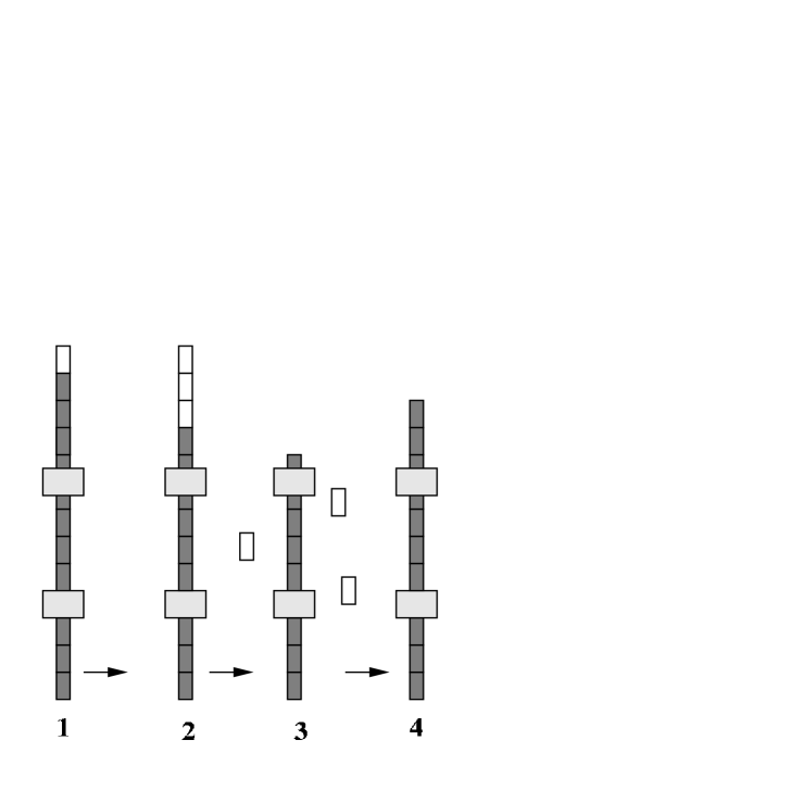
Figure 2: A schematic illustration of the dynamics of our model. The dark squares are the T-tubulin units and the white squares are the hydrolysed D-tubulin units. The large filled squares represent the microtubule-associated proteins. In (1), hydrolysis of the microtubule has started from the top end, which spreads to the bottom (2), and untimately leads to the D-tubulin units falling off the polymer. But the de-polymerization is arrested in (4) by the MAP, which promotes further polymerization.

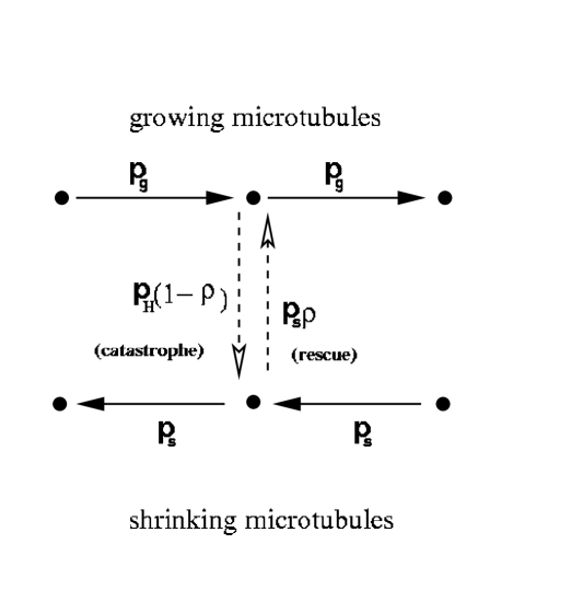
Figure 3: A schematic illustration of the various rates in the microtubule dynamics. Mirotubules make the transition between growing and shrinking states with rates which depend on the MAP density.

In this model, we assume that microtubules are thin rigid rods nucleating from the microtubule-organizing center, which is very often the centrosome(Fig.1). The three-dimensional structure of microtubules is ignored in our model. The centrosome contains nucleation sites for a microtubule, and nucleation takes place at vacant sites at a rate $\nu$. The microtubule grows by adding tubulin subunits at a rate $p_{g}$, and tubulin units inside the microtubule are stochastically hydrolyzed at a rate $p_{H}$. A microtubule will start de-polymerizing when the T-tubulin at its growing end is hydrolyzed to D-tubulin ref.3 ; ref.14 ; ref.15 . The shrinkage takes place at a rate $p_{s}$, which is the probability per unit time to lose a subunit. It is generally assumed that the de-polymerization process will continue along the length of the microtubule, until the shrinking end encounters a patch of T-tubulin in the interior. In our model, however, we assume that a microtubule in shortening state will continue to shrink (irrespective of the state of tubulin in the interior) until the de-polymerizing end encounters a MAP, which are present along the microtubule. This simplification helps focus on the role of MAPs in the microtubule dynamics. We further assume that MAPs also assist in the polymerization process by acting as polymerization sites along a microtubule. For further simplification, we assume the presence of an excess of free tubulin in solution, so that the dynamics of the tubulin concentration can be largely ignored. We also assume that the nucleation sites in the centrosome are spaced sufficiently far apart so that the effective interaction between microtubules through local depletion and enhancement of concentration of free tubulin is insignificant. A schematic illustration of the dynamics of our model is given in Fig.2, and a schematic illustration of the various rates of the model is shown in Fig.3.

It is helpful to note the typical experimental values of the various parameters in our model. We refer to recent experimental work ref.13 for most of the parameter values. Nucleation of microtubules in the centrosome was seen to occur at a rate of $\nu\simeq$ 5-6/min in vivo ref.13 . The velocity of growth of growing microtubules observed is $v_{g}\approx 20\mu m/min$. The rate of addition of tubulin dimers ($p_{g}$) is determined from $v_{g}$ as follows. A tubulin dimer has length $\approx 8nm$. Since there are 13 protofilaments of T-dimers in a single microtubule, each tubulin contributes a length of $\delta\approx 0.6nm$ to the microtubule. Thus, the rate of addition of tubulin dimers would be $p_{g}=v_{g}/\delta\simeq 0.55\times 10^{3}s^{-1}$. Using similar reasoning, the rate of loss of tubulin can be calculated from the measured velocity of shrinkage in shortening microtubules. This turns out be $p_{s}=v_{s}/\delta\approx 0.82\times 10^{3}s^{-1}$.

The rate of hydrolysis is a difficult parameter to measure, and is not as well known as the other rates. However, a wide range of values, 0.25-25/min has been reported ref.2 ; ref.14 ; ref.16 ; ref.17 . The typical values of the density $\rho$ of MAP used in injection experiments are estimated to be of the order $10^{-2}$ ref.18 ; ref.19 .

III Mean-Field Rate Equations

In this section, we analyze the mean-field rate equations for the time evolution of the probability distribution of the lengths of microtubules. Since our basic aim is to study the character of an assembly of microtubules, we resort to a statistical description. The most appropriate quantity to study in this perspective is the length distribution $p(l,t)$, which is the fraction of nucleation sites which has a microtubule of length $l$ at time $t$. The presence of MAP is taken into account through a mean-field density variable $\rho$, whose local fluctuations in space is ignored (The effect of these fluctuations are explicitly studied in numerical simulations presented in Sec.4). The MAPs change the microtubule dynamics by modifying the rates of shrinkage and hydrolysis, as seen below. It is also convenient to classify the entire set of microtubules into two: growing and shrinking microtubules (as was done in ref.15 ). Consequently, the complete length distribution $p(l,t)$ can also be split as follows.

$$p(l,t)=p_{+}(l,t)+p_{-}(l,t)$$ (1)

where $p_{+}(l,t)$ is the fraction of microtubule in growing state at any time $t$, and $p_{-}(l,t)$ is the fraction in shrinking state at time $t$. The rate of change of $p_{+}(l,t)$ is described by the following equation (for $l\geq 2$):

$$\frac{\partial p_{+}(l,t)}{\partial t}=p_{+}(l-1,t)p_{g}+p_{-}(l+1,t)\rho p_{s}-p_{+}(l,t)[p_{g}+p_{H}(1-\rho)]~{}~{}~{}~{};~{}~{}~{}l\geq 2$$ (2)

The significance of each term easily follows from the model description in Sec.2. The first two terms represent gain events, where a microtubule of length $l$ in growing state is created at time $t$. In particular, the second term describes the transition between a microtubule in a shrinking state to a growing state, and so

$$\nu_{r}=\rho p_{s}$$ (3)

is the rate of rescue in our model. We note that in our model $\nu_{r}\to 0$ as $\rho\to 0$, which is in agreement with the assumptions of our model. (However, in experiments, microtubules have been observed to undergo rescue under in vitro conditions in the absence of MAP. Our assumption here is that the MAP significantly increases the rescue frequency, which would otherwise be negligible). The last two terms represent the loss events where a microtubule of length $l$ either adds a tubulin to increase its length, or undergoes hydrolysis to transform into shrinking state. The latter is an event of catastrophe, and so the corresponding rate in our model is

$$\nu_{c}=p_{H}(1-\rho).$$ (4)

Both the rates of catastrophe and rescue are parameters which are measured in experiments. We also note that for microtubules of unit length, the gain event in $p_{+}(1,t)$ is nucleation, rather than polymerization, so that its equation is

$$\frac{\partial p_{+}(1,t)}{\partial t}=\nu R(t)+p_{-}(2,t)\rho p_{s}-p_{+}(1,t)[p_{g}+p_{H}(1-\rho)]$$ (5)

where $R(t)=1-\sum_{l=1}^{\infty}[p_{+}(l,t)+p_{-}(l,t)]$ is the fraction of vacant sites in the lattice at time $t$. The equation for $p_{-}(l,t)$ is,

$$\frac{\partial p_{-}(l,t)}{\partial t}=p_{+}(l,t)p_{H}(1-\rho)+p_{-}(l+1,t)p_{s}(1-\rho)-p_{-}(l,t)p_{s}~{}~{}~{};~{}~{}l\geq 1$$ (6)

The equations Eq.(2) and Eq.(6) are supplemented by the boundary condition for $p(l,t)$, which is,

$$lim_{l\to\infty}p(l,t)=0$$ (7)

We now proceed to look for the solution for these coupled set of rate equations. As a first step, we look for the steady state solution by putting the time derivatives to zero in Eq.(2) and Eq.(6).

III.1 The steady state:

In the steady state, it is reasonable to assume that both the distributions $p_{+}(l)$ and $p_{-}(l)$ (the time dependence has been dropped since we are looking at steady state solutions now) have the same dependence on $l$. Further, it is easily seen from the equations that the steady state solution has an exponential form, which is easily determined by substituting the trial functions

$$p_{+}(l)=Ae^{-\lambda l}~{}~{}~{};~{}~{}~{}p_{-}(l)=\gamma p_{+}(l)$$ (8)

in the steady state equations. In the trial solution, $\lambda$ and $\gamma$ are two unknown constants which need to be determined, and $A$ is the normalization factor. Upon substitution in Eq.(8) we find the following equations for the unknown constants $\lambda$ and $\gamma$.

$$p_{g}[e^{\lambda}-1]+\gamma p_{s}\rho e^{-\lambda}=p_{H}(1-\rho)=p_{s}\gamma[1-(1-\rho)e^{-\lambda})]$$

from which we determine the unknown constants $\lambda$ and $\gamma$ as follows.

$$\lambda=log[(1+\frac{p_{H}}{p_{g}})(1-\rho)]~{}~{}~{}~{}~{};~{}~{}\gamma=\frac{p_{g}+p_{H}}{p_{s}}(1-\rho)$$ (9)

Clearly, from the boundary condition in Eq(7), the solution is meaningful only if $\lambda>0$, and this implies that $\rho<\rho_{c}$, where

$$\rho_{c}=\frac{p_{H}}{p_{g}+p_{H}}$$ (10)

It turns out that $\rho_{c}$ is a critical value of MAP density, below which growth is bounded and the length distribution of microtubule is stationary. The typical values of $\rho_{c}$ can be easily estimated using the known values of $p_{H}$ and $p_{g}$. For example, keeping $p_{g}\simeq 0.55\times 10^{3}s^{-1}$ and changing $p_{H}$ from $\simeq$ 3/min to 300/min (which are close to in vivo estimates) gives $\rho_{c}$ in the interval $\sim 10^{-4}-10^{-2}$. This suggests that a very small MAP to tubulin ratio might be enough to stabilize microtubules against depolymerization.

The steady state solution discussed above is not valid when $\rho\geq\rho_{c}$, and so the solution for the rate equations has to be found explicitly for this case.

III.2 The unbounded growth regime

When $\rho>\rho_{c}$, growth becomes unbounded. Although the exact solution of the evolution equations in this regime is hard to find, it is helpful to note that under usual experimental conditions the growth and shrinkage rates far exceed the hydrolysis rate, i.e.,$p_{H}$ is small in comparison with $p_{g}$ and $p_{s}$. If we further assume that we work in the regime where the MAP density is high, i.e., $\rho\simeq 1$, then all the terms in the rate equations which contain $p_{H}$ can be neglected in comparison with the other terms. Further analytic progress is now possible by converting the finite difference equations into differential equations (in the limit $l\gg 1$). This is done by formally expanding $p_{\pm}(l,t)$ in its derivatives (see the appendix for a discussion on this point) as the series, $p_{\pm}(l\pm 1,t)=p_{\pm}(l,t)\pm\frac{\partial p_{\pm}}{\partial l}+\frac{1}{2}\frac{\partial^{2}p_{\pm}}{\partial l^{2}}$. After substitution, we arrive at the following differential equation for $p_{-}(l,t)$.

$$\frac{\partial p_{-}(l,t)}{\partial t}=\frac{p_{s}}{2}(1-\rho)\frac{\partial^{2}p_{-}(l,t)}{\partial l^{2}}+p_{s}(1-\rho)\frac{\partial p_{-}(l,t)}{\partial l}-p_{-}(l,t)p_{s}\rho$$ (11)

Let us now define the re-scaled time $\tau=\rho p_{s}t$ and the new variables $D=\frac{1-\rho}{2\rho}$ and $v=\frac{1-\rho}{\rho}$, in terms of which Eq.(11) is re-cast as

$$\frac{\partial p_{-}(l,\tau)}{\partial t}=D\frac{\partial^{2}p_{-}(l,\tau)}{\partial l^{2}}+v\frac{\partial p_{-}(l,\tau)}{\partial l}-p_{-}(l,\tau)$$ (12)

This equation is easily solved by substituting $p_{-}(l,\tau)=e^{-\tau}g(l,\tau)$, upon which we find that $g(l,\tau)$ satisfies the equation $\frac{\partial g}{\partial\tau}=D\frac{\partial^{2}g}{\partial l^{2}}+v\frac{\partial g}{\partial l}$, which is the well-known equation for diffusion of a particle in one dimension, with a drift term. The solution of this equation (apart from the trivial solution $g(l,\tau)=0$) has the form(up to a proportionality factor),

$$g(l,\tau)=\frac{1}{\sqrt{D\tau}}e^{-\frac{(l+v\tau)^{2}}{4D\tau}}$$ (13)

However, this solution is not physically reasonable since the mean length decreases with time as $\langle l\rangle=-v\tau$. It follows that in this limit, the solution for Eq.(11) is the trivial solution i.e, $p_{-}(l,t)\simeq 0$. The equation for $p_{+}(l,t)$ in the same limit is,

$$\frac{\partial p_{+}(l,\tau)}{\partial t}=\frac{p_{g}}{2}\frac{\partial^{2}p_{+}(l,\tau)}{\partial l^{2}}-p_{g}\frac{\partial p_{+}(l,\tau)}{\partial l}$$ (14)

which, again, is the diffusion equation with a drift term, whose solution is (up to a constant)

$$p_{+}(l,t)=\frac{1}{\sqrt{t}}e^{-\frac{(l-p_{g}t)^{2}}{2p_{g}t}}$$ (15)

We see that in the limits $p_{H}\ll p_{s}$ and $\rho\simeq 1$, the length distribution of growing microtubules is a Gaussian at all times, and the mean value increases linearly with time as $\langle l\rangle\approx p_{g}t$. Furthermore, in this limit, almost all the microtubules are in the growing state.

Although it is possible at this stage to look for a perturbative solution of the evolution equations Eq.(11) and Eq.(14) with $\frac{p_{H}}{p_{s}}$ as the pertrubation parameter, we have not attempted this here. Rather, in the next subsection, we determine the mean length as a function of time exactly, and shows that it agrees with the prediction of Eq.(15) in the limit $p_{H}\ll p_{s}$.

III.3 The average length of microtubules

In order to study the time evolution of the average length in the unbounded growth regime, it is convenient to define the following quantities:

$$Q_{+}(t)=\sum_{l=1}^{\infty}p_{+}(l,t)$$ (16)

which is the fraction of microtubule in growing state, irrespective of length, and

$$Q_{-}(t)=\sum_{l=1}^{\infty}p_{-}(l,t)$$ (17)

is the fraction of microtubule in shrinking state, irrespective of length. The time evolution of $Q_{+}(t)$ can be found by performing a sum of Eq. (2) over all $l\geq 2$ and adding Eq.(5).The result is

$$\frac{dQ_{+}(t)}{dt}=\nu R(t)-p_{H}(1-\rho)Q_{+}(t)+\rho p_{s}[Q_{-}(t)-p_{-}(1,t)]$$ (18)

For $Q_{-}(t)$, we perform a sum over Eq.(6) over all $l\geq 1$, and find that

$$\frac{dQ_{-}(t)}{dt}=p_{H}(1-\rho)Q_{+}(t)+p_{s}(1-\rho)[Q_{-}(t)-p_{-}(1,t)]-p_{s}Q_{-}(t)$$ (19)

where $R(t)=1-Q_{+}(t)-Q_{-}(t)$. The average length of microtubule at time $t$ is defined as

$$\langle l\rangle(t)=\sum_{l=1}^{\infty}l[p_{+}(l,t)+p_{-}(l,t)]$$ (20)

The rate of change of $\langle l\rangle$ with time may be expressed in terms of $Q_{+}(t)$ and $Q_{-}(t)$, since each growing microtubule grows by an amount $p_{g}$ and each shrinking microtubule shrinks by an amount $p_{s}$ per unit time. It follows that

$$\frac{d\langle l\rangle}{dt}=Q_{+}(t)p_{g}-Q_{-}(t)p_{s}$$ (21)

To calculate $Q_{+}(t)$ and $Q_{-}(t)$ from Eq.(18) and Eq.(19), let us first assume that $p_{-}(1,t)\ll Q_{-}(t)$. This assumption is valid in the unbounded growth regime, where the mean length increases with time, and hence the peak of the distribution is expected to shift toward larger and larger times (note the shifting Gaussian we found in the last section). The result is a closed set of equations for $Q_{+}(t)$ and $Q_{-}(t)$, which has the form

$$\frac{dQ_{+}(t)}{dt}=\nu(1-Q_{+}-Q_{-})-\alpha Q_{+}+\beta Q_{-}$$ (22)

and

$$\frac{dQ_{-}(t)}{dt}=\alpha Q_{-}-\beta Q_{+}$$ (23)

where $\alpha=p_{H}(1-\rho)$ and $\beta=\rho p_{s}$. We take the initial condition to be $Q_{+}(0)=\nu$ and $Q_{-}(0)=0$. The general solution for the above set of equations is

$$Q_{-}(t)=\frac{\alpha}{(\alpha+\beta)}+\frac{\alpha\nu(1-(\alpha+\beta))}{(\alpha+\beta)(\alpha+\beta-\nu)}e^{-(\alpha+\beta)t}-\frac{\alpha(1-\nu)}{(\alpha+\beta-\nu)}e^{-\nu t}$$ (24)

and

$$Q_{+}(t)=\frac{\beta}{\alpha+\beta}+\frac{\alpha\nu(1-(\alpha+\beta))}{(\alpha+\beta)(\alpha+\beta-\nu)}e^{-(\alpha+\beta)t}+\frac{\alpha(1-\nu)(\nu-\beta)}{(\alpha+\beta-\nu)}e^{-\nu t}$$ (25)

We note that the exponential terms vanish at sufficiently late times, and so the asymptotic forms of $Q_{+}(t)$ and $Q_{-}(t)$ are,

$$Q_{+}(t)\to\frac{p_{s}\rho}{p_{s}\rho+p_{H}(1-\rho)}~{}~{}~{}~{}~{};~{}~{}~{}t\to\infty$$

$$Q_{-}(t)\to\frac{p_{H}(1-\rho)}{p_{s}\rho+p_{H}(1-\rho)}~{}~{}~{}~{};~{}~{}~{}t\to\infty$$ (26)

Thus, even in the unbounded growth phase, a finite fraction of microtubule will be in the shrinking state. After substituting Eq.(26) in Eq.(21), we find that

$$\frac{d\langle l\rangle}{dt}\approx\frac{p_{s}[p_{g}\rho-p_{H}(1-\rho)]}{\rho p_{s}+p_{H}(1-\rho)}~{}~{}~{}~{};~{}~{}~{}t\to\infty$$ (27)

For unbounded growth, we need $\frac{d\langle l\rangle}{dt}>0$, for which the condition $\rho>\rho_{c}$, where $\rho_{c}$ is defined in Eq.(10). This calculation confirms that $\rho_{c}$ is the critical MAP density above which microtubules exist in a phase of sustained growth. In the limit $p_{H}\ll p_{s}$, we see that $\langle l\rangle\simeq p_{g}t$, which is one of the results we had derived in the last subsection.

III.4 Comparison with experiments

At this stage, it is worthwhile to compare our predictions (although based on a very simple model) with experimental observations regarding the effect of MAPs on microtubulesref.18 ; ref.19 . We specifically refer to experiments by Dhamodharan and Wadsworth ref.19 where MAPs were microinjected into BSC-1 cells and their effects on growth of microtubules, in particular, the changes in catstrophe and rescue frequencies, were studied. When 0.1 mg/ml of MAP-2 was added to the cells, the proportion of MAP to tubulin in the polymerized state was estimated to be nearly 1:25, or $\rho\simeq 0.04$. Increasing the MAP concentration 10-fold was observed to decrease the catastrophe frequency from 0.05 ($\pm 0.02$)$s^{-1}$ to 0.02 ($\pm 0.003$)$s^{-1}$, i.e., by a factor of nearly 0.4 after neglecting the experimental error. According to Eq. (4), increasing $\rho$ by a factor of 10, from 0.04 to 0.4, would decrease the catastrophe frequency by a factor of 0.625, which is in resonably good agreement with the experimental value. Furthermore, according to Eq. (4), the catastrophe rate in the absence of MAP is simply the hydrolysis rate $p_{H}$, which may be calculated from the same equation using experimental data for $\nu_{c}$ and $\rho$. The data for $\rho=0.4$ (which has greater accuracy) gives $p_{H}\approx 0.033s^{-1}$, which is, again, in reasonably good agreement with the experimental value of 0.043 ($\pm 0.01$) $s^{-1}$. The effects of MAP on the rescue frequency is more subtle, since rescue would occur in cells even in the absence of MAP, which is not taken into account in our model.

IV NUMERICAL SIMULATIONS

In this section, we discuss the results of our numerical simulations of the microtubule assembly. Since our model neglects any effective interaction between growth of neighboring microtubules due to local depletion of ligand concentration, the geometry of the system, and the spacing between individual microtubules is unimportant in the simulation. For simplicity, the cell interior is imagined as a rectangular box, where the base forms the substrate for nucleation of microtubules ref.15 . The microtubules grow in the direction perpendicular to the base until they hit the boundary.

The next step in the simulation procedure is to divide the box into a grid array of dimensions $L\times L\times H$, where $L$ is the length of the side of the substrate and $H$ is the height. As we had mentioned before, the lattice spacing in the substrate is unimportant as long as it is sufficiently large that direct interaction between neighboring microtubules could be ignored (henceforth, we shall always assume that this condition is satisfied). The lattice spacing in the direction of growth ($z$-axis) is the length of one tubulin dimer, which, after taking into account the number of protofilaments, is equivalent to $\delta z\simeq 0.6nm$. For the time evolution, we choose Monte Carlo step as equivalent to $\delta t\simeq 10^{-3}s$. With this timescale, the probability of a microtubule growing by one unit per MC step is nearly 0.55, and the probability that a tubulin unit is lost in one MC step is nearly 0.82, from the rates discussed in Sec. 2. In other words, the time scale has been chosen such that growth and shrinkage of microtubules are stochastic events, in accordance with the rate equations. For the lattice size, we chose $L=100$ and $H=500$.

The tubulin density in polymerized state at each point in space is represented using a density index $\phi({\bf r},z,t)$, where ${\bf r}$ is the substrate co-ordinate, $z$ is the position in the direction of growth and $t$ is time in units of MC steps. At $t=0$, we start with a substrate free of microtubule, i.e., $\phi({\bf r},z,0)=0$. We do not explicitly keep track of the density of free tubulin in the solution. The density index $\phi({\bf r},z,t)$ takes three values: $\phi({\bf r},z,t)=+1$ represents T-tubulin, $\phi({\bf r},z,t)=-1$ represents D-tubulin and $\phi({\bf r},z,t)=0$ implies that the site is empty. A string of $\phi({\bf r},z,t)\neq 0$ at any ${\bf r}$, for $1\leq z\leq l$ is a microtubule of length $l$. For $z=1$, $\phi({\bf r},z,t)$ changes from 0 to $+1$ with probability $\nu$ per MC step at all ${\bf r}$ and $t$. This is the nucleation event. For any $z>1$, this transition takes place with probability $p_{g}$, which is a polymerization event where a new T-tubulin dimer is added to the microtubule. The location of MAP in the lattice is specified through another density index $\chi({\bf r},t)$, which takes the value 1 or 0 depending on whether there is a MAP molecule at the lattice site (r,z) at time t. At all times, we distribute the MAPs at random throughout the lattice with mean density $\rho$. We do not take into account the diffusion of MAPs in solution explicitly. Rather, when microtubules grow from the substrate, they assimilate the MAPs along their length and release them randomly such that the mean density remains $\rho$ at all times. We assume here that the binding and release of MAP take place over time scales much less than one 1MC step in the simulation (which is equivalent to $10^{-3}$ seconds), so that, at each time step, the microtubule assembly has a different MAP configuration.

In all our simulations, the rates of growth and shrinkage were fixed as $p_{g}=0.55$ and $p_{s}=0.82$, which are the experimental values quoted in Sec.2. For reasons we shall shortly discuss, the hydrolysis rate was fixed at a value higher than the typical estimates, i.e, we chose $p_{H}=0.5$ (which would translate into a hydrolysis rate of $\approx 3\times 10^{4}$/minute). We also chose a high nucleation rate ($\nu=1$), for two reasons: to increase the occupancy of the lattice so as to improve the statistics, and to reduce the duration of the early-time regime of growth (where the exponential factors in Eq..(24) and Eq..(25) would ne non-negligible). The chosen values of $p_{H}$ and $p_{g}$ gives a convenient value of the critical MAP density, $\rho_{c}\simeq 0.47$ (which was the primary reason for choosing a high $p_{H}$).

We measured the length distribution and average length of microtubule assembly for three values of $\rho$, 0.1, 0.3 and 0.6. We chose the first two values to be below $\rho_{c}$, where we expect bounded growth (steady state distribution) and the last value is above $\rho_{c}$, where growth is expected to be unbounded. The results for probability distribution of lengths are given in Figs. 4-6, and the result for time evolution of the average length in the unbounded regime is displayed in Fig.7. In Fig. 4 and 5, we observe that, as predicted by the rate equation analysis, the solution is exponential, but the measured value of $\lambda$ differs from the mean-field prediction. This is presumably due to the spatial fluctuations in the MAP density, which is ignored in the mean-field analysis. In Fig.6, we find that the length distribution of microtubules in the unbounded regime closely resembles a Gaussian function with a mean value shifting with time. This is in accordance with the results of rate equation analysis in Sec. 3 (although in the simulations $p_{H}$ and $p_{s}$ are of the same order of magnitude). In Fig.7, we confirm that the mean length in the unbounded regime follows a linear dependence on time, again in agreement with the analysis in Sec.3.

V SUMMARY AND CONCLUSIONS

In this work, we have presented a simple theoretical model of stabilization of microtubules due to microtubule-associated proteins. We have shown that when the density of MAP is reduced below a critical value, the length distribution of the microtubule assembly undergoes a significant change. Whereas in one phase (at high MAP density) the microtubules extend throughout the cell, in the other phase they have an exponentially decaying length distribution with a finite average length. It is interesting to note that this transition is similar to the transition at mitosis in real cells, where phosphorylation of MAPs by agents such as the metaphase promoting factor (MPF)ref.10 leads to a weakening of their binding to the microtubules, and a consequent change in length distribution. We have also shown that the critical ratio of MAP to polymerized tubulin required for a transition to the ’cell-spanning’ phase can be as low as 1:1000 under in vivo conditions. Thus, our conclusion is that even a very small concentration of MAP can sustain unlimited growth of microtubules, which is in qualitative agreement with experiments ref.18 .

There are still many open questions regarding the effect of MAPs on microtubule dynamics in cells. In fact, MAPs which inhibit polymerization have also been identified recently ref.11 . It would be interesting to include such MAPs also in our model and look for the consequences of competition between the effects of two kinds of MAP. Moreover, our prediction of the existence of a critical MAP density which differentiates between two distinct growth regimes for microtubules could be verified in future experiments. Lastly, our model could be still improved by including effects of local fluctuations in the concentrations of MAP and tubulin. In particular, it would be interesting to ask in the context of such an improved model whether there exists subpopulations of microtubules in one growth regime, while the over-all growth behavior of the whole population is in the other regime. These are some of the questions we would like to address in the future.

VI ACKNOWLEDGMENTS

The authors would like to gratefully acknowledge the Carilion Biomedical Institute for providing the funding which allowed this work to be carried out. One of us (B.G) would like to thank Prof. R. A. Walker for helpful discussions.

APPENDIX

In this appendix, we outline the scheme by which the difference equations Eq..(2) and Eq..(6) are converted to partial differential equations Eq..(11) and Eq..(14). We first define the first derivative in a symmetric way by taking the average over right and left derivatives.

$$\frac{\partial p_{\pm}}{\partial l}\equiv\frac{[p_{\pm}(l+1)-p_{\pm}(l)]+[p_{\pm}(l)-p_{\pm}(l-1)]}{2}$$

We note that the second and third terms cancel each other, so we arrive at

$$\frac{\partial p_{\pm}}{\partial l}\equiv\frac{p_{\pm}(l+1)-p_{\pm}(l-1)}{2}$$

For the second derivative, we use the familiar Euler discretization scheme, i.e,

$$\frac{\partial^{2}p_{\pm}}{\partial l^{2}}\equiv p_{\pm}(l+1)+p_{\pm}(l-1)-2p_{\pm}(l)$$

After solving these two equations together, we arrive at the expression

$$p_{\pm}(l\pm 1,t)=p_{\pm}(l,t)\pm\frac{\partial p_{\pm}}{\partial l}+\frac{1}{2}\frac{\partial^{2}p_{\pm}}{\partial l^{2}}$$

Figure 1: A schematic illustration of microtubules inside the cell. The filled circle is the microtubule-organizing center, which is very often the centrosome.

Figure 4: Probability distribution of microtubule length when $\rho=0.1$. We observe bounded growth with exponential distribution of lengths as predicted by the rate equations. The unit of time in this plot is one second. $f(l)\propto e^{-\lambda l}$ is a fit function where $\lambda\approx 0.79$, which differs somewhat from the mean-field prediction of Eq..(9), which gives $\lambda\simeq 0.54$.

Figure 5: The figure shows the probability distribution of microtubule lengths when $\rho=0.3$. In this case, growth is again bounded, but the length scales reached by the microtubule is longer than before. The unit of time in this plot is one second. $f(l)\propto e^{-\lambda l}$ is a fit function, with $\lambda\approx 0.49$. The mean-field prediction for $\lambda$ given by Eq .(9) is nearly 0.28.

Figure 6: The figure shows the probability distribution of microtubule lengths when $\rho=0.6$ at three different times. The growth is unbounded since $\rho>\rho_{c}$. The peak of the distribution shifts to the right with increasing time, which shows that the average length increases with time. The unit of time in this figure is one second and length is measured in units of $\delta$ = 0.6nm.

Figure 7: The plot shows the average length of the microtubule assembly increasing linearly with time for $\rho=0.6$, which is above $\rho_{c}$. The straight line is a linear fit. Time is measured in seconds and length is measured in units of $\delta$ = 0.6nm.

References

- (1) D. Nelson, Mechanics of the Cell (Cambridge University Press) (2000).
- (2) H.P.Erickson and E.T. O’Brien, Ann.Rev.Biophys.Biomol.Struc. 21, 145-166 (1992)
- (3) T. Mitchison and M. Kirschner, Nature 312, 299-304.(1984a)
- (4) T.J. Mitchison, Science 21, 1044-47 (1993).
- (5) R.A. Walker, E.T. O’Brien, N.K. Pryer, M.F.Soboeiro and W.A.Voter, J. Cell. Biol.107, 1437-48 (1988).
- (6) H. Flyvbjerg, T. E.Holy and S. Leibler, Phys. Rev. E. 54, 5538-60 (1996).
- (7) D.K.Fygenson , H. Flyvbjerg, K. Sneppen, A. Libchaber and S. Leibler, Phys. Rev. E 51, 5058-63 (1995).
- (8) R. Valle, Proc.Natl.Acad.Sci. USA. 77,3206-3210 (1980).
- (9) E. Karsenti and I. Vernos, Science 294, 543-547 (2001).
- (10) I. Vernos and E. Karsenti, Dynamics of Cell division, S.A. Endow and D.M. Glover(Eds), (Oxford University Press)(1998) .
- (11) J.Howard, A. A. Hyman, Nature 422, 753-758 (2003).
- (12) L. Cassimeris and C. Spittle, Int. Rev. Cytol. 210, 163-226 (2001).
- (13) Y.A. Komarova, I. A. Vorobjev and G. G. Borisy, J. Cell Science 115, 3527-39 (2001).
- (14) M.F. Carlier , R. Meiki. , D. Pantalini. , T. L. Hill and Y. Chen, Proc. Natl. Acad. Sci. USA. 84, 5257-61 (1987).
- (15) M. Dogterom and S. Leibler, Phy. Rev. Lett. 70, 1347-50 (1993).
- (16) M.F. Carlier and D. Pantaloni, Biochemistry 20, (1981).
- (17) A. Desai and T. J. Mitchison, Annu. Rev. Cell. Dev. Biol. 13, 83-117 (1997).
- (18) N.K. Pryer, R.A. Walker, V.P Skeen, B.D. Bourns, M.F. Soboeiro and E.D. Salmon, J.Cell Sci. 103, 965-976, (1992).
- (19) R. Dhamodharan and P. Wadsworth, J .Cell Sci. 108, 1679-1689 (1995).