A Quasispecies on a Moving Oasis

Abstract

A population evolving in an inhomogeneous environment will adapt differently to different regions. We study the conditions under which such a population can maintain adaptations to a particular region when that region is not stationary, but can move. In particular, we study a quasispecies living near a favorable patch (“oasis”) in the middle of a large “desert.” The population has two genetic states, one of which which conveys a relative advantage while in the oasis at the cost of a disadvantage in the desert. We consider the population dynamics when the oasis is moving, or equivalently some form of “wind” is blowing the population away from the oasis. We find that the ratio of the two types of individuals exhibits sharp transitions at particular oasis velocities. We calculate an extinction velocity, and a switching velocity above which the dominance switches from the oasis-adapted genotype to the desert-adapted one. This switching velocity is analagous to the quasispecies mutational error threshold. Above this velocity, the population cannot maintain adaptations to the properties of the oasis.

Spatial inhomogeneities in the environment are often essential to understanding the dynamics of natural populations. Populations may for example be confined to limited reserves or live in an environment with gradients in resources or large-scale inhomogeneities in habitability. The evolution of a population in an inhomogeneous environment is particularly interesting. When individuals move over the environment sufficiently rapidly relative to the length scale of the inhomogeneities, they may all see and adapt to an “averaged” environment. When this is not true, however, the dynamics can be much more complex. Some individuals may randomly see primarily one part of the range while others see other parts. The population in the distant future will likely be dominated by the descendents of a few exceptionally lucky individuals in the present, who will have seen an unusually favorable subset of the set of possible environments. Thus it is not at all clear a priori exactly how different regions of the environment will influence the evolution.

In this paper, we consider a simple environment with two regions, a favorable “oasis” in a large less favorable (or unfavorable) “desert.” The favorable area could be realized as a game reserve, a region of favorable climactic conditions, or a patch of light, among other things. Provided that the favorable region is stationary and sufficiently large, a population will adapt to the special properties of this region. However, in many cases the oasis will move at some typical speed $v$, for example due to seasonal weather patterns or human intervention. (Equivalently, the population could be blown across the oasis at speed $v$ by some form of “wind”). In this situation, there is a velocity beyond which the population will not be able to maintain adaptations to the properties of the oasis. Rather, the evolution will be dominated only by the desert environment. We focus in this paper on calculating this velocity, which we call the “switching velocity.”

Recent work has considered the dynamics, though not the evolution, of a population being blown by some form of convective “wind” across a nonuniform environment. In these models, the equation for the population density at a point $(\vec{x},t)$ is

$$\frac{\partial{c(\vec{x},t)}}{\partial{t}}=D\nabla^{2}c-\vec{v}\cdot\nabla c+r(\vec{x})c,$$ (1)

where $D$ is the diffusion constant, $\vec{v}$ is the drift velocity, and $r(\vec{x})$ is the growth rate. This equation thus describes a population multiplying in response to some spatially heterogeneous environment while diffusing and drifting. It can be analyzed using techniques adapted from an analysis of non-Hermitian Schroedinger-like operators 252 ; 255 . A nonlinear saturation term can be added, and is important for some purposes.

Ref. 111 examines this model in two dimensions in the case where $r(\vec{x})$ is random, with only short-range correlations. In the limit of small $v$ ($v\ll v_{F}\equiv 2\sqrt{aD}$, where $a$ is the average of $r(x)$), the population is dominated by a few colonies that grow up around “hot spots,” regions which happen to have higher growth rates than surrounding areas. As $v$ increases, individual colonies on less prosperous hot spots are blown away in a series of “delocalization” transitions. In the limit of large $v$ all organisms are blown away from individual hot spots and convect across the environment. At long times, the population is dominated by those individuals that happened to take very special paths through the random environment, travelling through a disproportionate number of the hot spots. Thus this is an example of a system in which a typical individual will evolve in response to a very special subset of the environment.

In subsequent work, Dahmen et. al. examined the transition between the small and large $v$ regimes by looking at a model of a single “hot spot” 230 . These authors took the growth rate $r(\vec{x})$ to be large within a small hot spot, or “oasis,” and smaller (and possibly negative) in the surrounding “desert.” They analyzed the dynamics near the extinction and delocalization velocities, where the population is blown off of the oasis. Their predictions have been qualitatively confirmed by recent experiments on Bacillus subtilis growth 231 .

In this paper, we extend this work to consider the dynamics of a population of multiple types of individuals in a desert-oasis environment. In particular, we consider a quasispecies model with two types of individuals. Thus $c(\vec{x},t)$ becomes a two-vector

$$\mbox{\boldmath${c}$}(\vec{x},t)=\left(\begin{array}[]{c}c_{1}(\vec{x},t)\\ c_{2}(\vec{x},t)\end{array}\right),$$ (2)

and $r(\vec{x})$ becomes a two-by-two matrix with diagonal elements specifying the growth rates of the two genotypes and off-diagonal elements specifying the mutation and back-mutation rates. Genotype $1$ represents the population of some “ideal” genome sequence, while type $2$ represents all other less ideal sequences. There is mutation back and forth between the two, typically with a mutation rate away from the ideal sequence greater than the mutation rate towards it. Without any spatial variation, (i.e. with $r(x)$ independent of $x$), this is a simple quasispecies model. A few recent papers have examined other versions of a spatial quasispecies model, with many different possible types of individuals representing all possible Hamming distances from the ideal sequence 245 ; 227 . Here, we focus on a simple two-type spatial model, although it is straightforward to generalize our results.

We assume that the population $c_{1}$ has some gene or sequence which conveys an advantage in the environment of the oasis, but has an overall cost which makes it disadvantageous in the desert. The population $c_{2}$ consists of all individuals who have lost the function of the gene by one or more mutations. Individuals of type $1$ are thus those that have adapted to the special properties of the oasis, while type $2$ individuals are desert-adapted.

We examine the population dynamics as we change the velocity $v$. We find two important transitions. When the growth rate in the desert is negative, there is an extinction velocity $v_{e}$ where the entire population goes extinct. When the genotype $2$ desert growth rate is positive, there is a “switching” velocity $v_{s}$ where the behavior of the population changes dramatically. Below this velocity the population (particularly within the oasis) is dominated by genotype $1$. Above it, the oasis-adapted genotype is outcompeted, genotype $2$ dominates, and $c_{1}/c_{2}\to 0$ at long times. This transition is a velocity-driven analog of the classical mutational error threshold in non-spatial quasispecies models altmeyerref1 ; altmeyerref2 ; altmeyerref5 .

These results have interesting implications. If the oasis represents some part of a species’ habitat, the switching velocity is simply how quickly this can move before the species can no longer maintain adaptations to the properties of this aspect of its range. Our analysis is also a first step towards understanding the spatial quasispecies model in a random environment, where the population does not evolve in response to the averaged environment but rather in response to a different, highly selective subset of the environment.

The outline of this paper is as follows. In section I we give a detailed description of our model. In section II we outline the calculation of the critical velocities and the behavior of the populations in the different regimes. In section III we compare our analytical results with computer simulations. Finally, in section IV we discuss the main biological implications of these calculations.

I Model

We consider a population with two types of individuals whose densities are described by

$$\mbox{\boldmath${c}$}(\vec{x},t)=\left(\begin{array}[]{c}c_{1}(\vec{x},t)\\ c_{2}(\vec{x},t)\end{array}\right).$$ (3)

The dynamics is exponential growth (or decay) with diffusion and convection

$$\frac{\partial{\mbox{\boldmath${c}$}(\vec{x},t)}}{\partial{t}}=D\nabla^{2}\mbox{\boldmath${c}$}-\vec{v}\cdot\vec{\nabla}\mbox{\boldmath${c}$}+\mbox{\boldmath${\mathcal{R}}$}(\vec{x})\mbox{\boldmath${c}$},$$ (4)

where $\mbox{\boldmath${\mathcal{R}}$}(\vec{x})$ is a two-by-two matrix. We are primarily concerned with the extinction and delocalization transitions. Thus for the bulk of our analysis, we neglect the possibility of a nonlinear saturation term. In section IV.1 we discuss the consequences of such a nonlinearity.

We define the growth and death rates of individuals of type $i$ within the oasis to be $\alpha_{i}$ and $\gamma_{i}$ respectively. Outside the oasis, the growth and death rates are defined to be $\beta_{i}$ and $\delta_{i}$. The mutation rate from type 1 to type 2 is defined to be $\mu_{1}$, and the back-mutation rate is $\mu_{2}$. Based on these definitions, the matrix $\mbox{\boldmath${\mathcal{R}}$}(\vec{x})$ is given by

$$\mbox{\boldmath${\mathcal{R}}$}(\vec{x})=\left(\begin{array}[]{cc}\alpha_{1}-\gamma_{1}-\mu_{1}\alpha_{1}&\mu_{2}\alpha_{2}\\ \mu_{1}\alpha_{1}&\alpha_{2}-\gamma_{2}-\mu_{2}\alpha_{2}\end{array}\right)$$ (5)

inside the oasis and similarly (with $\alpha\to\beta$ and $\gamma\to\delta)$ in the desert.

For simplicity, we assume that the growth rates within the desert and the oasis are the same, i.e. $\alpha_{i}=\beta_{i}$. The desert is less hospitable because of a higher death rate, not a lower growth rate. This simplifies the analysis but is not a serious limitation; the results for $\alpha\neq\beta$ are straightfoward to calculate by the same methods. We next define $a_{i}\equiv\alpha_{1}-\gamma_{1}$ and $b_{i}\equiv\beta_{i}-\delta_{i}$. For convenience we also assume that $a_{1}=\alpha_{1}$ and $a_{2}=\alpha_{2}$ (i.e. $\gamma_{1}=\gamma_{2}=0$). It is easy to relax this assumption, but the results more transparent with it in place. These simplifications yield the matrix

$$\mbox{\boldmath${\mathcal{R}}$}(\vec{x})=\left(\begin{array}[]{cc}a_{1}-\mu_{1}a_{1}&\mu_{2}a_{2}\\ \mu_{1}a_{1}&a_{2}-\mu_{2}a_{2}\end{array}\right)\qquad\textrm{(inside oasis)}$$ (6)

in the oasis and similarly in the desert,

$$\mbox{\boldmath${\mathcal{R}}$}(\vec{x})=\left(\begin{array}[]{cc}b_{1}-\mu_{1}a_{1}&\mu_{2}a_{2}\\ \mu_{1}a_{1}&b_{2}-\mu_{2}a_{2}\end{array}\right)\qquad\textrm{(outside oasis)}.$$ (7)

We assume that $a_{1}>b_{1}$ and $a_{2}>b_{2}$, so that we have a beneficial oasis and a harmful desert. We further assume that $a_{1}>a_{2}$ and $b_{2}>b_{1}$ (which also implies $a_{2}>b_{1}$) so that genotype $1$ is better in the oasis and genotype $2$ is better in the desert. Absent these inequalities, one or the other type will unequivocally dominate the population (up to the mutational error threshold) independent of the drift velocity. In that case, we can ignore the inferior type at long times and the problem reduces to that studied in 230 . Our assumptions imply that individuals of type 1 have some function that conveys an advantage inside the oasis, at the cost of a disadvantage elsewhere. Our analysis will determine whether or not this function can be maintained in the face of mutational pressure when the oasis is moving at velocity $v$.

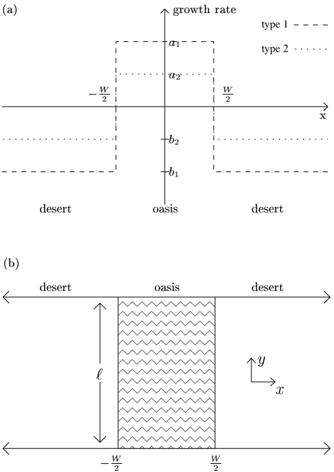
Figure 1: (a) shows the one-dimensional system we consider, for the case of a deadly desert. The dashed line is the growth rate of genotype 1, the dotted line the growth rate of genotype 2. This is an approximation to the two-dimensional system shown in (b), valid when the initial conditions are uniform in the $y$ direction or the time is greater than $\ell^{2}/D$.

We could of course make any number of assumptions about the geometry of the desert and the oasis. We will consider for simplicity a one-dimensional system with an oasis of width $W$ in the middle of an infinite desert, as depicted in figure 1a. This analysis also describes the long time behavior of the two-dimensional system with geometry as described by figure 1b. If the initial conditions are uniform in the $y$ direction, the one-dimensional system of figure 1a is equivalent to the two-dimensional system of figure 1b. If the conditions are nonuniform, the two become equivalent after a time of order $\ell^{2}/D$ 230 . More complicated geometries are certainly possible, and we discuss these briefly in section IV.2.

We assume throughout that differential equations are an adequate representation of these biological processes. We neglect discreteness in population number, which may have some importance near the extinction transition. The effects of discreteness may be analyzed using the methods of 46 ; 54 ; 56 ; 58 ; 59 ; 60 ; 61 .

II Calculation of the Population Dynamics

We analyze our model using the non-Hermitian methods of Refs. 252 ; 255 ; 111 . We first rewrite our system in the form

$$\frac{\partial{\mbox{\boldmath${c}$}(x,t)}}{\partial{t}}=\mbox{\boldmath${\mathcal{L}}$}\mbox{\boldmath${c}$},$$ (8)

where ${\mathcal{L}}$ is given by $\mbox{\boldmath${\mathcal{L}}$}=\mbox{\boldmath${\mathcal{L}}$}_{in}\theta(W-|x|)+\mbox{\boldmath${\mathcal{L}}$}_{out}\theta(|x|-W)$, and $W$ is the width of the oasis. The function $\theta(y)=1$ if $y\geq 0$ and $0$ otherwise, and

$$\mbox{\boldmath${\mathcal{L}}$}_{in} = \left(\begin{array}[]{cc}D\partial_{x}^{2}-v\partial_{x}+a_{1}-\mu_{1}a_{1}&\mu_{2}a_{2}\\ \mu_{1}a_{1}&D\partial_{x}^{2}-v\partial_{x}+a_{2}-\mu_{2}a_{2}\end{array}\right),$$ (11)

$$\mbox{\boldmath${\mathcal{L}}$}_{out} = \left(\begin{array}[]{cc}D\partial_{x}^{2}-v\partial_{x}+b_{1}-\mu_{1}a_{1}&\mu_{2}a_{2}\\ \mu_{1}a_{1}&D\partial_{x}^{2}-v\partial_{x}+b_{2}-\mu_{2}a_{2}\end{array}\right).$$ (14)

${\mathcal{L}}$ is non-Hermitian, but we can diagonalize it with a system of left and right eigenfunctions $\mbox{\boldmath${\phi}$}_{n}^{R}(x)$ and $\mbox{\boldmath${\phi}$}_{n}^{L}(x)$, with their (common) eigenvalues $\Gamma_{n}$. These eigenfunctions (which we also call “states”) satisfy the orthonormality condition

$$\int\mbox{\boldmath${\phi}$}_{m}^{L}(x)\cdot\mbox{\boldmath${\phi}$}_{n}^{R}(x)dx=\delta_{mn}.$$ (15)

Using this result, we can write the initial condition as a linear superposition of the right eigenfunctions, i.e. $\mbox{\boldmath${c}$}(x,t=0)=\sum_{n}c_{n}\mbox{\boldmath${\phi}$}_{n}^{R}(x)$, where

$$c_{n}=\int d^{d}x\mbox{\boldmath${\phi}$}_{n}^{L}(x)\cdot\mbox{\boldmath${c}$}(x,t=0).$$ (16)

We can then immediately write down the solution valid for all times, namely

$$\mbox{\boldmath${c}$}(x,t)=\sum_{n}c_{n}\mbox{\boldmath${\phi}$}_{n}^{R}(x)e^{\Gamma_{n}t}.$$ (17)

This result has a clear biological interpretation. Initially, the population is in some particular arrangement, expressible as a linear combination of the different eigenfunctions. This combination will necessarily include the eigenfunction corresponding to the largest $\Gamma_{n}\equiv\Gamma_{gs}$ (which is always real) endnote2 . This eigenfunction is special, and we refer to it as the “ground state” endnote4 . As time passes, the population distribution looks more and more like the ground state. This distribution will grow (or die out) exponentially with rate $\Gamma_{gs}$. The other $\mbox{\boldmath${\phi}$}_{m}^{R}$ may be important initially, but since they grow more slowly than the ground state, they soon become irrelevant. Thus understanding the ground state function and its eigenvalue are the key to understanding the long time behavior of the population.

It remains to solve for the eigenfunctions and eigenvalues $\mbox{\boldmath${\phi}$}_{n}^{L}(x),\mbox{\boldmath${\phi}$}_{n}^{R}(x)$, and $\Gamma_{n}$. For the case $v=0$, the solution is straightforward and will be discussed in detail below. For nonzero $v$, we make use of the fact that the eigenfunctions of $\mbox{\boldmath${\mathcal{L}}$}_{v=0}$ are related to the eigenfunctions of ${\mathcal{L}}$ by an “imaginary gauge transformation” 111 . That is, if $\mbox{\boldmath${\phi}$}_{n,v=0}^{R}(x)$ is a right eigenfunction of $\mbox{\boldmath${\mathcal{L}}$}_{v=0}$ with eigenvalue $\Gamma_{n}$, then

$$\mbox{\boldmath${\phi}$}^{R}_{n,v}(x)=e^{vx/2D}\mbox{\boldmath${\phi}$}_{n,v=0}^{R}(x)$$ (18)

is a right eigenfunction of ${\mathcal{L}}$, with eigenvalue

$$\Gamma_{n}^{v}=\Gamma_{n}^{v=0}-\frac{v^{2}}{4D},$$ (19)

as can be verified by allowing ${\mathcal{L}}$ to act on $\mbox{\boldmath${\phi}$}_{n}^{R}$. Similar expressions hold for $\mbox{\boldmath${\phi}$}^{L}_{n,v}$. The eigenvalues $\Gamma_{n}^{v=0}$ are all real. Thus, eigenfunctions for $v>0$ are very similar to the eigenfunctions for $v=0$. The genotype 1 versus genotype 2 composition of the states is not altered at all. The only change is that the wind causes a distortion of the population in the direction of the wind, and the growth rates of the states shift downward “rigidly” (i.e. independent of $n$) by an amount $\frac{v^{2}}{4D}$.

However, this procedure works only for small $v$. To see this, consider the behavior of the eigenfunctions as $x\to\infty$. We expect (and will soon verify) that the $v=0$ eigenfunctions far from the oasis decay exponentially,

$$\phi_{n,v=0}\sim e^{-\kappa_{n}|x|}.$$ (20)

Thus for $v>0$,

$$\phi_{n}^{R}\sim e^{vx/2D-\kappa_{n}|x|}.$$ (21)

When $v<2D\kappa_{n}$, the eigenfunctions vanish at infinity, as they should. However, for $v>2D\kappa_{n}$, this function blows up at infinity, which is unreasonable. The correct eigenfunctions have a different character when $v>2D\kappa_{n}\equiv v^{*}_{n}$.

Ref. 252 shows that the transition at $v_{n}^{*}$ is a delocalization of the corresponding eigenfunction. For $v<v^{*}_{n}$, the eigenfunctions are localized around the oasis, but for $v>v^{*}_{n}$ they are delocalized. This makes intuitive sense. For small velocities, the population will tend to cluster around the oasis, but for larger wind velocities it gets blown off the oasis and must live by drifting across the desert. The behavior of the eigenvalues $\Gamma_{n}$ near this delocalization transition is striking. Up to $v^{*}_{n}$, the eigenvalue $\Gamma_{n}^{v}$ is simply equal to $\Gamma_{n}^{v=0}-\frac{v^{2}}{4D}$, but beyond this point this relation no longer holds. Instead, $\Gamma_{n}$ jumps off the real axis at $v^{*}_{n}$, becoming complex, and the eigenfunctions become broad delocalized states extending through the desert 252 ; 255 ; 111 . We denote the value of $\Gamma_{n}$ at which this occurs by $\Gamma^{*}_{n}$. As we continue to increase $v$ above $v_{n}^{*}$, the real part of $\Gamma_{n}$ stays approximately constant, although the imaginary part does change. From the gauge transformation relationship, we have $\Gamma_{n}^{*}=\Gamma^{v=0}_{n}-\frac{(v^{*}_{n})^{2}}{4D}$. However, as we will see, the structure of the $n$-dependence of $v_{n}$ and $\Gamma_{n}$ is such that there are only two different values of $\Gamma_{n}^{*}$. This is a crucial point. In our problem, the states will divide into those dominated by genotype 1 and those dominated by genotype 2. As we will show, states dominated by genotype $1$ delocalize at $\Gamma_{1}^{*}=\langle r_{1}\rangle$, the spatial average growth rate of the first genotype, which up to finite size effects is just $b_{1}$. $\Gamma_{2}^{*}=\langle r_{2}\rangle\approx b_{2}$ plays the same role for states dominated by the second genotype. By our assumptions about the parameters, $\Gamma_{2}^{*}>\Gamma_{1}^{*}$. An example of eigenvalue spectra for several values of $v$ is given in figure 2.

Figure 2: An example of eigenvalue spectra, shown here for $3$ values of $\bar{v}=\frac{v}{v_{F}}\equiv\frac{v}{2\sqrt{Da_{1}}}$ with $\bar{a}_{1}=1,\bar{b}_{1}=-1,\bar{a}_{2}=0.6,\bar{b}_{2}=-0.6,\mu_{1}=0.01,\mu_{2}=0.001$, and $\bar{D}=0.25$, where the overbars indicate the non-dimensionalized parameters discussed in Appendix C. To allow easy distinction from the $\bar{v}=0$ results, the localized $\bar{v}=0.9$ eigenvalues have been shifted slightly upwards. Note the rigid shift of the localized eigenvalues (those on the real axis) to the left as we increase $\bar{v}$. This is highlighted by the three $\bar{v}=0$ states marked by upwards arrows, which for $\bar{v}=0.9$ are shifted into the three states marked by downards arrows. The two (and only two) delocalization transitions $\bar{\Gamma}_{1}^{*}\approx-1$ and $\bar{\Gamma}_{2}^{*}\approx-0.6$ are also clearly visible. Note that these transition points, and all the delocalized states, do not shift to the left as $\bar{v}$ increases. On the left half of the spectrum (omitted from the figure), the delocalized eigenstates form closed loops, an artifact of the computational discretization used to produce this figure.

Each localized state has some particular $\Gamma_{n}^{v=0}$, and for nonzero $v$ its eigenvalue becomes $\Gamma_{n}=\Gamma_{n}^{v=0}-\frac{v^{2}}{4D}$. As $v$ increases, $\Gamma$ decreases until the state delocalizes, at $\Gamma_{1}^{*}$ for those states dominated by type 1 and at $\Gamma_{2}^{*}$ for those states dominated by type 2. We will see that the ground state for $v=0$ is dominated by genotype 1. As $v$ increases there comes a critical point when this ground state eigenvalue $\Gamma_{gs}$ crosses $\Gamma_{2}^{*}$. Beyond this point it is no longer the ground state. Rather, the delocalized genotype-2 dominated state with eigenvalue $\Gamma_{2}^{*}$ has the highest $\Gamma$, and this state determines the population dynamics. We call this critical velocity the “switching velocity,” where the dominance switches from genotype 1 to genotype 2. This switch is a type of quasispecies transition, caused not by exceeding a mutation rate error threshold, but by exceeding a critical velocity. This reasoning is illustrated in figure 3.

Figure 3: A single eigenvalue spectrum, with the genotype-1 and genotype-2 dominated states distinguished. This is just the $\bar{v}=0.9$ spectrum from figure 2 above. Note the state with the largest Re$(\Gamma)$ (i.e. the ground state) is a genotype-1 dominated state. This $\bar{v}$ is just below the extinction velocity, so $\Gamma_{gs}$ is just above the extinction threshhold, indicated by the dashed vertical line at $\Gamma=0$. As $\bar{v}$ increases, all of the localized (real) states move to the left until they enter either the left parabola of delocalized states (for genotype-1 dominated states) or the right parabola of delocalized states (for genotype-2 dominated states). Thus as $\bar{v}$ increases $\Gamma_{gs}$ will soon pass through $0$ at the “extinction velocity”. However, the delocalized states do not shift to the left as $\bar{v}$ increases. Thus as $\bar{v}$ increases further, $\Gamma_{gs}$ will eventually pass through $\Gamma_{2}^{*}$, indicated by the center vertical line. Once this happens, the largest Re$(\Gamma)$ no longer belongs to the original genotype-1 dominated state, but rather to a genotype-2 dominated delocalized state. The critical velocity at which this occurs is the “switching velocity.” In this example, since $\Gamma_{2}^{*}<0$, the switching velocity is higher than the extinction velocity, and is therefore biological uninteresting. However, if we had $\Gamma_{2}^{*}>0$, the spectrum would look identical, except it would be shifted to the right. We would then have $\Gamma_{2}^{*}>0$, and hence there would always be states above Re$(\Gamma)=0$. Thus there would be no extinction velocity, and the switching velocity would be biologically relevant.

If the growth rate for genotype 2 in the desert is negative, then $\Gamma_{2}^{*}<0$. The switching behavior will then be difficult to observe experimentally, as both genotypes will be going extinct when it happens. In this case, the biologically interesting transition occurs at the “extinction” velocity where the growth rate of the ground state passes through $0$. Beyond this velocity, all the states have negative growth rate, so neither genotype can survive. When the growth rate for genotype 2 in the desert ($b_{2}$) is positive, the switching velocity becomes biologically relevant. In this case, there is no extinction velocity. This is because the delocalized states do not shift to lower $\Gamma$ as $v$ increases, and at least one genotype-2 dominated delocalized state has eigenvalue $\Gamma_{2}^{*}\approx b_{2}>0$. Intuitively, this makes sense because the population, dominated by genotype 2, can survive in the desert at arbitrarily large velocities.

II.1 Solution for the Eigenvalues and Eigenfunctions

In order to carry out the analysis sketched above, we must solve for the $v=0$ eigenvalues and eigenfunctions, and determine the values of $\Gamma_{1}^{*}$ and $\Gamma_{2}^{*}$. It is possible to do this exactly, and an outline of this calculation is presented in Appendix A. However, it is more straightforward and instructive to first examine the solutions for $\mu_{1}=\mu_{2}=0$, and then use perturbation theory to find the results for small $\mu_{1}$ and $\mu_{2}$.

II.1.1 The $\mu_{1}=\mu_{2}=0$ Solution

We first examine the system for $\mu_{1}=\mu_{2}=0$. In this case, the two types of individuals are completely independent. The problem reduces to that studied in 230 . We use the imaginary gauge transformation to eliminate the velocity, and focus on the $v=0$ eigenvalues and eigenstates. We then have to solve the eigenvalue equation

$$\mbox{\boldmath${\mathcal{L}}$}_{v=0}\phi_{n}^{i,v=0}=\Gamma_{n}^{i,v=0}\phi_{n}^{i,v=0}.$$ (22)

This problem is formally equivalent to the square well problem in quantum mechanics qmbook . The $v=0$ right eigenstates are of the form

$$\mbox{\boldmath${\phi}$}_{n}^{1,v=0}=\left(\begin{array}[]{c}\psi_{n}^{1}\\ 0\end{array}\right),\qquad\mbox{\boldmath${\phi}$}_{n}^{2,v=0}=\left(\begin{array}[]{c}0\\ \psi_{n}^{2}\end{array}\right),$$ (23)

where

$$\psi_{n}^{i}=\left\{\begin{array}[]{ll}A_{n}^{i}e^{\kappa_{n}^{i}x}&\mathrm{for}\quad x<-W/2\\ B_{n}^{i}e^{ik_{n}^{i}x}+C_{n}^{i}e^{-ik_{n}^{i}x}&\mathrm{for}\quad-W/2<x<W/2\\ G_{n}^{i}e^{-\kappa_{n}^{i}x}&\mathrm{for}\quad x>W/2.\end{array}\right.$$

Note that the index $i$ indicates the genotype that dominates the state. Substituting this ansatz into the eigenvalue equation leads to

$$\Gamma_{n}^{i,v=0}=D(\kappa_{n}^{i})^{2}+b_{i}=-D(k_{n}^{i})^{2}+a_{i}.$$ (24)

We proceed by requiring that ${\phi}$ and its first derivative be continuous at $x=\pm W/2$, which determines the constants $A,B,C$, and $G$ up to an overall normalization and yields a transcendental equation to determine $\Gamma$. This analysis is carried out in detail in 230 . The essential result is that provided the oasis is wide enough that a typical individual gives birth many times while diffusing across it, the ground state eigenvalue can be approximated as $\Gamma^{v=0,\mu=0}_{gs}\approx a_{1}$, with a corresponding eigenfunction that is entirely genotype 1 and localized largely within the oasis. We will use this approximation throughout the rest of this paper endnote3 . We can also calculate the position of the delocalization transitions $\Gamma_{n}^{i*}$. These are defined as the amount by which the $v=0$ eigenvalue $\Gamma_{n}^{i,v=0}$ is shifted by the delocalization velocity $v_{n}^{i*}$. We thus have $\Gamma_{n}^{i*}=\Gamma_{n}^{i,v=0}-\frac{(v_{n}^{i*})^{2}}{4D}=\Gamma_{n}^{i,v=0}-D(\kappa_{n}^{i})^{2}$. Using Eq. (24), we find $\Gamma_{n}^{i*}=b_{i}$. Note that, as claimed above, this $\Gamma_{n}^{i*}$ is independent of $n$ and depends only on $i$. Thus there are two and only two delocalization threshholds, one corresponding to each genotype.

II.1.2 Perturbation Theory in $\mu_{1}$ and $\mu_{2}$

We can now examine the results for nonzero mutation rates $\mu_{1},\mu_{2}>0$ by using a non-Hermitian version of time-independent perturbation theory from quantum mechanics qmbook . We require that $\mu_{1}$ and $\mu_{2}$ be small, specifically that $\frac{\mu_{i}a_{i}}{a_{1}-a_{2}},\frac{\mu_{i}a_{i}}{b_{2}-b_{1}}\ll 1$. The details of the calculation are described in Appendix B. The eigenstates now all involve both genotypes, although those that began as genotype $1$ states remain dominated by this type, and vice versa. More precisely, we have

$$\mbox{\boldmath${\phi}$}_{n}^{1,v=0,R}=\left(\begin{array}[]{c}\psi_{n}^{1}\\ \frac{\mu_{1}a_{1}}{a_{1}-a_{2}}\psi_{n}^{2}\end{array}\right),$$ (25)

for a genotype-1 dominated localized state, and

$$\mbox{\boldmath${\phi}$}_{n}^{2,v=0,R}=\left(\begin{array}[]{c}\frac{\mu_{2}a_{2}}{b_{2}-b_{1}}\psi_{n}^{1}\\ \psi_{n}^{2}\end{array}\right)$$ (26)

for a genotype-2 dominated delocalized state, where $\psi_{n}^{1}$ and $\psi_{n}^{2}$ are given in section II.1.1. Note that we focus on genotype-1 dominated localized states and genotype-2 dominated delocalized states because no other state can dominate the dynamics in any regime. The eigenvalues are also shifted. The eigenvalues for genotype-1 dominated localized states become

$$\Gamma_{n}^{1,v=0}=\Gamma_{n}^{i,v=0,\mu=0}-\mu_{1}a_{1}+\frac{\mu_{1}a_{1}\mu_{2}a_{2}}{a_{1}-a_{2}},$$ (27)

while the genotype-2 dominated delocalized states have eigenvalues

$$\Gamma_{n}^{2,v=0}=\Gamma_{n}^{2,v=0,\mu=0}-\mu_{2}a_{2}+\frac{\mu_{1}a_{1}\mu_{2}a_{2}}{b_{2}-b_{1}},$$ (28)

plus higher order terms in $\mu_{1}$ and $\mu_{2}$.

II.2 Critical Velocities

We can now calculate the critical velocities at which the dynamics changes qualitatively. There are two relevant cases. For $b_{2}<0$ neither delocalization transition occurs at positive $\Gamma$ because neither genotype can survive in the desert. Thus the switching velocity, though it exists formally, is biologically irrelevant. The extinction velocity $v_{e}$ is the velocity where the ground state eigenvalue passes through zero. Below $v_{e}$ a genotype-1 dominated population can multiply but above this velocity the population must go extinct. This velocity is defined by $\Gamma_{gs}^{v_{e}}=\Gamma_{gs}^{v=0}-\frac{v_{e}^{2}}{4D}=0$, which using Eq. (27) gives

$$v_{e}=2\sqrt{(Da_{1})}\left[1-\frac{\mu_{1}}{2}\right],$$ (29)

valid to first order in $\mu_{1}$ and $\mu_{2}$. Note that for $\mu_{1}=0$, we have $v_{e}=v_{F}\equiv 2\sqrt{Da_{1}}$, the Fisher velocity for genotype $1$.

For $b_{2}>0$ there is no extinction velocity, as genotype 2 can survive at any velocity. However, there is a switching velocity $v_{s}$ where the population shifts from being mostly genotype 1 to mostly genotype 2. This occurs when the growth rate of the genotype-1 dominated ground state passes through $\Gamma_{2}^{*}=b_{2}-\mu_{2}a_{2}+\frac{(\mu_{2}a_{2})^{2}}{b_{2}-b_{1}}$. By a similar calculation we find

$$v_{s}=2\sqrt{D(a_{1}-b_{2})}\left[1-\frac{1}{2}\frac{\mu_{1}a_{1}}{a_{1}-b_{2}}+\frac{1}{2}\frac{\mu_{2}a_{2}}{a_{1}-b_{2}}\right],$$ (30)

also valid to first order in $\mu_{1}$ and $\mu_{2}$. As mentioned above, this switching velocity is a sort of quasispecies transition. As the velocity increases passes this critical threshold, the population can no longer maintain the “ideal” sequence, even if it is below the mutational error threshold. This switching velocity is also well-defined for $b_{2}<0$, but will be difficult to observe because $v_{s}>v_{e}$. We can easily calculate the second-order corrections to both $v_{e}$ and $v_{s}$ (see Appendix B).

Figure 4: A comparison of the critical velocities $\bar{v}_{e}$ and $\bar{v}_{s}$ from the simulations to the analytical result, as a function of $\mu_{1}=10\mu_{2}$. The analytical result is shown as a dashed line for $\bar{v}_{s}$ and a dotted line for $\bar{v}_{e}$. Here we have $\bar{a}_{1}=1$, $\bar{a}_{2}=0.6$, $\bar{b}_{1}=-1$, $\bar{b}_{2}=-0.6$, and $\bar{D}=0.25$, where the overbars indicate the dimensionless units described in Appendix C. This result is typical of such comparisons for other parameter values. For these parameters, we expect the perturbation calculation of the analytical result to be valid for $\mu_{1}\ll 0.4$. The slight overestimates of $\bar{v}_{e}$ and $\bar{v}_{s}$ by the analytic theory for small $\mu_{1}$ are due to finite size effects. The underestimate as $\mu_{1}$ grows beyond the range of our perturbation expansion is due to the importance of higher-order terms.

III Simulations

We use two different computational methods to test our analytic results. First, we use a lattice discretization of the Liouville operator ${\mathcal{L}}$ to calculate the eigenvalue and eigenfunction spectrum for particular sets of parameter values. This numerical work provides an aid to intuition and one check of the validity of our approximations. Second, we simulate the underlying discrete process, namely individuals multiplying and mutating at appropriate rates. This tests not just the results of our analysis, but also the overall applicability of continuous time differential equations to the real discrete populations we model.

III.1 Lattice Approximation to the Liouville Operator

We made several approximations in arriving at our analytical results, including an approximations for $\Gamma_{gs}$ and for the shifts in eigenvalues with $\mu_{1}$ and $\mu_{2}$. To test these approximations, we calculate the eigenvalue spectrum numerically. We discretize space, find the resulting discretized Liouville operator, and numerically diagonalize it for a particular set of parameters. The details of this method are described in Appendix C.

This approach allows us to determine the shifts in the growth rates as $\mu$ or $v$ is varied, and hence the critical velocities $v_{e}$ and $v_{s}$. We can compare these results to our analytical predictions, and therefore confirm our calculation of the critical velocities. This comparison for one particular set of parameters is shown in figure 4. Comparisons for other parameter values have been carried out, and give similar results. The eigenvalue spectra shown in figure 2 and figure 3 were also obtained in this way.

III.2 Simulations of the Discrete System

We can also simulate the underlying discrete process which inspired our formulation of the differential equations we analyze in this paper. We discretize space, placing individuals on a one-dimensional lattice which represents our environment. These individuals move around, proliferate, die, and mutate. We also impose a saturation term so that at long times the population distribution settles down to a steady state.

By comparing the steady state population profiles for different values of $v$, we determine $v_{e}$ or $v_{s}$. These results can then be compared to the analytical results. This comparison, for one particular set of parameters, is shown in figure 4. Note that this comparison is only for $v_{e}$, as for these parameter values $v_{s}$ is not biologically relevant and is thus impossible to observe with this type of simulation. The details of this method are described in Appendix D.

IV Discussion

To interpret our results, it is helpful to first consider the behavior of a non-spatial quasispecies model. We imagine a population living in a uniform environment whose conditions match those of the oasis. Genotype 1 grows more quickly, but there is a mutational pressure away from this “ideal” genotype. Mutation away from this sequence is typically expected to be much more frequent than mutation back, so it is common in such models to set $\mu_{2}=0$. It is then straightforward to calculate the composition of the population. We find that the equilibrium ratio of genotype $1$ to genotype $2$ individuals $q\equiv c_{1}/c_{2}$ is given by

$$q=\frac{(1-\mu_{1})a_{1}-a_{2}}{\mu_{1}a_{1}}.$$ (31)

Thus the ratio of species $1$ to $2$ decreases with increasing $\mu_{1}$ until $\mu_{1}$ reaches the critical “error threshold” for this quasispecies model. At this threshold, $\mu_{1}^{c}=\frac{a_{1}-a_{2}}{a_{1}}$, the “ideal” genotype can no longer survive and the population becomes completely dominated by genotype $2$. This is the most famous result of Eigen’s quasispecies model altmeyerref1 ; altmeyerref2 ; altmeyerref5 .

Our analysis finds that, in analogy to the quasispecies error threshold, in the spatial model there is a velocity threshold above which genotype $1$ is outcompeted by genotype $2$. This velocity, which we call the switching velocity $v_{s}$, is given by Eq. (30). If the growth rate of genotype 2 in the desert is positive, we can expect to see this behavior in a real system. Our model naturally also has the traditional error threshold; for $\mu_{1}>\frac{a_{1}-a_{2}}{a_{1}}$ and $\mu_{2}=0$, genotype $1$ is outcompeted by genotype $2$ regardless of $v$. It would be interesting to explore the interactions between the mutation-driven and velocity-driven quasispecies transitions. However, our analysis is based on the assumption of small mutation rates and thus focuses on the velocity-driven transition under the assumption that we are well away from the mutation-driven transition endnote1 . A qualitative phase diagram of the different velocity-driven transitions is given in figure 5.

Figure 5: A phase diagram showing the transitions as a function of $v$ and $b_{2}$. This figure accounts for the qualitative effects of a nonlinear saturation term.

Our model describes a number of important biological situations. The oasis could be a particularly favorable patch of the environment or a zone of favorable climactic conditions which is moving at a typical speed $v$ due to seasonal weather patterns or shifts in climate. A population can take advantage of this oasis by adapting to these conditions, but then will fare worse in the rest of the space. Our analysis explores how fast the oasis can move before the population can no longer maintain an adaptation to the favorable patch. Beyond this speed individuals may occasionally find themselves in the oasis but cannot adapt quickly enough to benefit.

Besides showing the existence of the velocity-driven quasispecies transition, our results make $5$ interesting biological predictions. We discuss each of these in turn.

(1) The overall population growth rate decreases as $v^{2}$ up to the critical velocity. The imaginary gauge transformation tells us that for $b_{2}<0$, the exponential growth rate of the population decreases as $\frac{v^{2}}{4D}$ until it goes extinct at $v_{e}=2\sqrt{a_{1}D}\left(1-\frac{\mu_{1}}{2}\right)$. For $b_{2}>0$ the exponential growth rate of the population decreases again by $\frac{v^{2}}{4D}$ until it reaches $v_{s}=2\sqrt{(a_{1}-b_{2})D}\left(1-\frac{\mu_{1}a_{1}}{a_{1}-b_{2}}+\frac{\mu_{2}a_{2}}{a_{1}-b_{2}}\right)$. Increasing the velocity further does not change the overall growth rate because a delocalized genotype $2$ population then dominates.

(2) Below the critical velocity, the genotype-1 dominated population will extend somewhat into the desert. The type-1 population will extend a typical distance $\xi=\frac{1}{\kappa_{gs}-\frac{v}{2D}}$ into the desert. From the relationship between $\kappa$ and $\Gamma$ we find that this typical distance is

$$\xi=\frac{2D}{2\sqrt{D(a_{1}-b_{1})}-v},$$ (32)

independent of the mutation rates. Note that this diverges as $(v_{c}-v)^{-1}$ as $v\to v_{c}$ from below, where $v_{c}\equiv 2\sqrt{D(a_{1}-b_{1})}$ is the velocity at which the type-1 dominated ground state eigenvalue $\Gamma_{gs}$ reaches its delocalization threshold $\Gamma_{1}^{*}$. This divergence will be difficult to observe in real biological systems because $v_{s}<v_{c}$.

(3) The ratio of the two genotypes is proportional to $\mu$. Below the switching velocity, the ratio of the number of type $2$ individuals to type $1$ approaches $\frac{\mu_{1}a_{1}}{a_{1}-a_{2}}$ at long times. Above the switching velocity, the ratio of type $1$ to type $2$ is $\frac{\mu_{2}a_{2}}{b_{2}-b_{1}}$ at long times. This result, however, is only true within the linear model. If we add a saturation term to the dynamics, this term will affect the long-time population ratios.

(4) The ratio of genotype 1 to genotype 2 is independent of $v$ except when crossing $v_{s}$. We might naively expect that as we increase $v$, the population gets driven more towards the desert, and thus the population shifts away from genotype $1$ towards genotype $2$. The gauge transformation ensures that this does not happen. Until we cross $v_{s}$, the ratio of genotypes in the ground state eigenfunction, and thus the population, remains constant. At $v_{s}$ there is a sharp transition and the ratio of the genotypes shifts radically in favor of genotype $2$. As we continue to increase the velocity, the ratio again remains constant. This result, however, is also only true within the linear model. A nonlinear saturation term “softens” the transition at $v_{s}$, as described in section IV.1.

(5) The “right” ratio of genotypes dominates exponentially. If the initial state of the population below the switching velocity is all type $2$, then type $1$ will take over exponentially with a rate equal to the difference between $\Gamma_{gs}$ and the dominant type $2$ eigenvalue. This rate is just $a_{1}-a_{2}-\mu_{1}a_{1}+\mu_{2}a_{2}$, and is independent of $v$. Similarly, if we begin with a type-$1$ dominated population above the switching velocity, the population will become dominated by genotype $2$ exponentially with rate $b_{2}-b_{1}-\mu_{2}a_{2}+\mu_{1}a_{1}$, again independent of $v$.

IV.1 Effects of a Nonlinearity

Thus far we have concentrated on purely linear systems, without much discussion of nonlinear terms which cause the population to saturate. This approximation is justified because the presence of a nonlinear saturation term will not affect the critical velocities. However, since all populations can be expected to saturate at some point, it is important to consider the general implications of such a nonlinearity.

In the discussion to this point, we have assumed that the eigenfunction with the largest growth rate will dominate the population, so that at long times we can neglect all but this dominant state. In the nonlinear case this is still roughly true. We can account for the effects of the nonlinearity by using mode couplings as in 111 , and anticipate that the fastest growing eigenfunction will suppress the others and dominate the population. There is, however, one important exception to this idea. For the problem considered here, the fastest-growing localized eigenfunction vanishes exponentially outside of the oasis, and hence will not suppress the growth of the fastest-growing delocalized eigenfunction. Thus below the switching velocity $v_{s}$, the population is not in fact completely dominated by genotype $1$. Rather, there is a genotype-$1$ dominated population inside the oasis and a genotype-$2$ dominated delocalized population in the desert. As we increase $v$ we decrease the growth rate of the localized type $1$ dominated state without changing the growth rate of the delocalized genotype $2$ dominated state. Since the overall population sizes are set by the growth rates and the nonlinear terms, this will lead to a shift in the overall population density from type 1 to type 2. Thus there will be some $v$-dependence in the genotype ratio even below $v_{s}$. Just above $v_{s}$, the fastest-growing delocalized eigenfunction will not completely suppress the fastest-growing localized eigenfunction, so similarly there will be some $v$-dependence above $v_{s}$. The transition at $v_{s}$ is thus softened by the presence of the nonlinearity. While the dominance will still shift at this critical velocity, the transition will have some width dependent on the saturation term.

The nonlinearity will also impose a maximum carrying capacity on the system. As the system approaches this carrying capacity, the growth rates will slow down. Thus if we start with an initial condition involving a population already near its carrying capacity, our analysis of the rate at whch the “right” genotype composition is established will be an overestimate. While the results regarding the switching and extinction velocities and genotype composition still hold, the dynamics of reaching the resulting steady states will be slower. Our results for the rates are based on the linearization of the nonlinear model around $c_{1}=c_{2}=0$, and so are valid as long as the ratio of the population to the carrying capacity is small compared to 1.

IV.2 Other Geometries

Many alternative geometries are clearly possible. One obvious choice is a circular oasis in an infinite desert, as considered in 230 . The primary effect of a nontrivial two-dimensional geometry is to change the eigenvalue spectrum. In particular, $\Gamma_{gs}$ and, if the desert is not infinite, $\Gamma_{2}^{*}$ will shift. The resulting change in the switching and extinction velocities will depend on the growth rates $a_{i}$ and $b_{i}$ and the linear size of the oasis $W$, but not on $\mu$. However, the qualitative behavior is unaffected. Furthermore, if $W$ is large compared to $\sqrt{D/a}$, the typical length an individual diffuses before giving birth (the precise requirement will vary with the specific geometry), this shift in critical velocities will vanish and the results will reduce to those calculated above.

Appendix A: Exact Solution for the $v=0$ System

It is straightforward, though tedious, to find the exact solution for the $v=0$ eigenfunctions and eigenvalues. We start with the ansatz

$$\mbox{\boldmath${\phi}$}^{R}=\left(\begin{array}[]{c}Ae^{-\kappa_{1}x}+Be^{-\kappa_{2}x}\\ Ce^{-\kappa_{1}x}+Ee^{-\kappa_{2}x}\end{array}\right),$$ (33)

for $\frac{W}{2}<x$,

$$\mbox{\boldmath${\phi}$}^{R}=\left(\begin{array}[]{c}Fe^{ik_{1}x}+Ge^{-ik_{1}x}+He^{ik_{2}x}+Ie^{-ik_{2}x}\\ Je^{ik_{1}x}+Ke^{-ik_{1}x}+Le^{ik_{2}x}+Me^{-ik_{2}x}\end{array}\right)$$ (34)

for $-\frac{W}{2}<x<\frac{W}{2}$, and

$$\mbox{\boldmath${\phi}$}^{R}=\left(\begin{array}[]{c}Ne^{\kappa_{1}x}+Oe^{\kappa_{2}x}\\ Pe^{\kappa_{1}x}+Qe^{\kappa_{2}x}\end{array}\right)$$ (35)

for $x<-\frac{W}{2}$, where the 16 parameters $A,B,C,E,F,G,H,I,J,K,L,M,N,O,P$, and $Q$ are constant coefficients. Demanding that this ansatz satisfy the eigenvalue equation yields a system of $12$ equations relating these constant coefficients, $\kappa,k$, and the eigenvalue $\Gamma$. We use $8$ of these equations to eliminate $8$ of the $16$ coefficients, and the remaining $4$ to determine $\kappa_{1},\kappa_{2},k_{1}$, and $k_{2}$ in terms of the eigenvalue $\Gamma$. We find that for small $\mu_{1}$ and $\mu_{2}$ ($\frac{\mu_{1}\mu_{2}b_{1}b_{2}}{(b_{1}-b_{2})^{2}}\ll 1$ and $\frac{\mu_{1}\mu_{2}a_{1}a_{2}}{(a_{1}-a_{2})^{2}}\ll 1$),

$$D\kappa_{1}^{2} = \Gamma-b_{2}+\mu_{2}a_{2}+\frac{\mu_{1}a_{1}\mu_{2}a_{2}}{b_{2}-b_{1}}$$ (36)

$$D\kappa_{2}^{2} = \Gamma-b_{1}+\mu_{1}a_{1}-\frac{\mu_{1}a_{1}\mu_{2}a_{2}}{b_{2}-b_{1}}$$ (37)

$$Dk_{1}^{2} = -\Gamma+a_{1}-\mu_{1}a_{1}+\frac{\mu_{1}a_{1}\mu_{2}a_{2}}{a_{1}-a_{2}}$$ (38)

$$Dk_{2}^{2} = -\Gamma+a_{2}-\mu_{2}a_{2}-\frac{\mu_{1}a_{1}\mu_{2}a_{2}}{a_{1}-a_{2}},$$ (39)

which serves to confirm our perturbation theory calculation. The expressions when $\mu_{1}$ and $\mu_{2}$ are not small are straightforward to calculate but unwieldy to write down.

We now demand that ${\phi}$ and $\frac{d{\mbox{\boldmath${\phi}$}}}{d{x}}$ be continuous at $x=\pm\frac{W}{2}$, yielding $8$ equations for the remaining $9$ unknowns ($8$ constant coefficients and $\Gamma$). These results lead to a transcendental equation for $\Gamma$, the solutions to which are the eigenvalues of the system. Choosing a particular eigenvalue from among these possible solutions, we can easily determine the remaining unknowns (up to an overall normalization) from the rest of the equations. By requiring

$$\int\mbox{\boldmath${\phi}$}^{L}(x)\cdot\mbox{\boldmath${\phi}$}^{R}(x)dx=1,$$ (40)

we determine the normalization, and thus the exact solution.

In practice, the transcendental equation for $\Gamma$ is quite complicated and we can only solve it numerically. However, this exact approach does provide a useful check to the discretized numerical solution described in section III. The most important result is the $\mu=0$ ground state eigenvalue $\Gamma^{\mu=v=0}_{gs}$. Provided that the oasis is much wider than the distance a typical individual diffuses before giving giving birth, we have $\Gamma_{gs}^{\mu=v=0}\approx a_{1}$ 230 .

Appendix B: Perturbation Theory in $\mu_{1}$ and $\mu_{2}$

We can use standard perturbation theory from quantum mechanics qmbook to determine the results for $\mu_{1},\mu_{2}>0$ from the $\mu_{1}=\mu_{2}=0$ solution. We first rewrite the Liouville operator as $\mbox{\boldmath${\mathcal{L}}$}_{v=0}=\mbox{\boldmath${\mathcal{L}}$}_{0}+\mbox{\boldmath${\mathcal{L}}$}_{1}$, where $\mbox{\boldmath${\mathcal{L}}$}_{1}$ is proportional to the (small) mutation rates $\mu_{1}$ and $\mu_{2}$, and

$$\mbox{\boldmath${\mathcal{L}}$}_{0} = \left(\begin{array}[]{cc}D\partial_{x}^{2}+r_{1}(x)&0\\ 0&D\partial_{x}^{2}+r_{2}(x)\end{array}\right),$$ (43)

$$\mbox{\boldmath${\mathcal{L}}$}_{1} = \left(\begin{array}[]{cc}-\mu_{1}a_{1}&\mu_{2}a_{2}\\ \mu_{1}a_{1}&-\mu_{2}a_{2}\end{array}\right),$$ (46)

where $r_{i}(x)=(a_{i}+\mu_{i}a_{i})\theta(W-|x|)+(b_{i}+\mu_{i}a_{i})\theta(|x|-W)$. We know the eigenvalues and eigenfunctions of $\mbox{\boldmath${\mathcal{L}}$}_{0}$ from section II and from 230 . For our purposes, all that is necessary is that the eigenfunctions are an orthonormal set of left and right functions $\mbox{\boldmath${\phi}$}_{n}^{L}$ and $\mbox{\boldmath${\phi}$}_{n}^{R}$.

From non-degenerate time-independent perturbation theory we find that the $\mu>0$ eigenvalues are related to the $\mu=0$ eigenvalues by the formula

$$\Gamma_{n} = \Gamma_{n}^{\mu=0}+\int\mbox{\boldmath${\phi}$}_{n}^{L}(x)\mbox{\boldmath${\mathcal{L}}$}_{1}\mbox{\boldmath${\phi}$}_{n}^{R}(x)dx+$$

$$+\sum_{m\neq n}\frac{\left(\int\mbox{\boldmath${\phi}$}_{m}^{L}(x)\mbox{\boldmath${\mathcal{L}}$}_{1}\mbox{\boldmath${\phi}$}_{n}^{R}(x)dx\right)\left(\int\mbox{\boldmath${\phi}$}_{n}^{L}(x)\mbox{\boldmath${\mathcal{L}}$}_{1}\mbox{\boldmath${\phi}$}_{m}^{R}(x)dx\right)}{\Gamma_{n}^{\mu=0}-\Gamma_{m}^{\mu=0}},$$

plus terms of third and higher order in $\mbox{\boldmath${\mathcal{L}}$}_{1}$ qmbook . Note that this result differs slightly from standard theory because $\mbox{\boldmath${\mathcal{L}}$}_{1}$ is non-Hermitian. The first-order term in ${\mathcal{L}}$ is straightforward to calculate. It is simply $-\mu_{i}a_{i}$ for states dominated by genotype $i$. The second-order term is more complicated, because the $\mu=0$ eigenfunctions are of the form

$$\mbox{\boldmath${\phi}$}_{n}^{R}=\left(\begin{array}[]{c}\psi_{n}^{1}\\ 0\end{array}\right)\quad\mathrm{or}\quad\mbox{\boldmath${\phi}$}_{n}^{R}=\left(\begin{array}[]{c}{0}\\ {\psi_{n}^{2}}\end{array}\right),$$ (48)

where the $\{\psi_{n}^{1}\}$ and $\{\psi_{m}^{2}\}$ each form an orthonormal set of eigenfunctions of the one-genotype problem. The $\psi_{n}^{1}$ and $\psi_{m}^{2}$ are almost, but not quite, orthonormal to each other.

In the approximation that these two sets of eigenfunctions are indeed orthonormal, the second order term for $\Gamma_{n}$ is easy to calculate. For genotype-1 dominated localized states, it is $\frac{\mu_{1}a_{1}\mu_{2}a_{2}}{a_{1}-a_{2}}$. For genotype-2 dominated delocalized states, it is $\frac{\mu_{1}a_{1}\mu_{2}a_{2}}{b_{2}-b_{1}}$. In the same approximation, the corrections to the eigenfunctions are given by

$$\mbox{\boldmath${\phi}$}_{n}^{1,v=0,R}=\left(\begin{array}[]{c}\psi_{n}^{1}\\ \frac{\mu_{1}a_{1}}{a_{1}-a_{2}}\psi_{n}^{2}\end{array}\right),$$ (49)

for a genotype-1 dominated localized state, and

$$\mbox{\boldmath${\phi}$}_{n}^{2,v=0,R}=\left(\begin{array}[]{c}\frac{\mu_{2}a_{2}}{b_{2}-b_{1}}\psi_{n}^{1}\\ \psi_{n}^{2}\end{array}\right)$$ (50)

for a genotype-2 dominated delocalized state.

These results, and the observation that $\Gamma_{gs}^{\mu=v=0}=a_{1}$ and $\Gamma_{2}^{*,\mu=v=0}=b_{2}$, allow us to calculate the critical velocities. To second order in $\mu_{1}$ and $\mu_{2}$, the extinction velocity is given by

$$v_{e}=2\sqrt{(Da_{1})}\left[1-\frac{\mu_{1}}{2}-\frac{\mu_{1}^{2}}{8}+\frac{\mu_{1}\mu_{2}a_{2}}{2(a_{1}-a_{2})}\right],$$ (51)

and the switching velocity is

$$v_{s} = 2\sqrt{D(a_{1}-b_{2})}\left[1-\frac{\mu_{1}a_{1}-\mu_{2}a_{2}}{2(a_{1}-b_{2})}-\frac{(\mu_{1}a_{1}-\mu_{2}a_{2})^{2}}{8(a_{1}-b_{2})^{2}}\right.$$ (52)

$$\left.+\frac{\mu_{1}a_{1}\mu_{2}a_{2}}{2(a_{1}-a_{2})(a_{1}-b_{2})}-\frac{\mu_{1}a_{1}\mu_{2}a_{2}}{2(b_{2}-b_{1})(a_{1}-b_{2})}\right].$$

The first order part of this result is quoted in section II above.

This perturbation expansion relies on the assumption that $\mu_{1}$ and $\mu_{2}$ are small. Specifically, we require

$$\frac{\mu_{i}a_{i}}{a_{2}-a_{1}}\ll 1\qquad\frac{\mu_{i}a_{i}}{b_{2}-b_{1}}\ll 1,$$ (53)

for $i=1,2$ for all of these results to be valid.

Appendix C: Lattice Approximation

Here we describe the details of the lattice approximation to the Liouville operator. We begin by discretizing space, replacing it by a regular lattice with lattice constant $\ell_{0}$. We define $c_{x}^{\alpha}$ to be the population of genotype $\alpha$ at the lattice point $x$. We then have to solve the eigenvalue equation

$$\frac{d{c_{x}^{\alpha}(t)}}{d{t}}=\sum_{x^{\prime},\alpha^{\prime}}\mbox{\boldmath${\mathcal{L}}$}(x,\alpha,x^{\prime},\alpha^{\prime})c_{x^{\prime}}^{\alpha^{\prime}}(t)=\Gamma c_{x}^{\alpha}(t).$$ (54)

The discretized version of the Liouville operator is

$${\mathcal{L}} = \frac{D}{\ell_{0}^{2}}\sum_{x}\sum_{\alpha=1}^{2}\left[e^{-\frac{v\ell_{0}}{2D}}|x\rangle^{\alpha}{}^{\alpha}{\langle}x+\ell_{0}|\right.$$ (55)

$$\left.+e^{\frac{v\ell_{0}}{2D}}|x+\ell_{0}\rangle^{\alpha}{}^{\alpha}{\langle}x|-2\cosh\left(\frac{v\ell_{0}}{2D}\right)|x\rangle^{\alpha}{}^{\alpha}{\langle}x|\right]$$

$$+\sum_{x}\left[U_{1}(x)|x\rangle^{1}{}^{1}{\langle}x|+U_{2}(x)|x\rangle^{2}{}^{2}{\langle}x|\right.$$

$$+\left.\mu_{1}a_{1}|x\rangle^{1}{}^{2}{\langle}x|+\mu_{2}a_{2}|x\rangle^{2}{}^{1}{\langle}x|\right],$$

where we have used the notation $|x\rangle^{\alpha}{}^{\beta}{\langle}y|$ to mean the tensor product of localized states corresponding to $c_{x}^{\alpha}$ and $c_{y}^{\beta}$. We define $U_{1}(x)=(a_{1}-\mu_{1}a_{1})\theta(W-|x|)+(b_{1}-\mu_{1}a_{1})\theta(|x|-W),$ and $U_{2}(x)=(a_{2}-\mu_{2}a_{2})\theta(W-|x|)+(b_{2}-\mu_{2}a_{2})\theta(|x|-W)$. We impose a finite size on the system $L$ (with periodic boundary conditions) and a finite width of the oasis $W$, with $W\ll L$.

In order for the lattice approximation to be valid, the lattice must be fine enough that variations in the eigenfunction $\phi$ between lattice points is small. This means we must require $\frac{\ell_{0}|\partial_{x}\phi_{n}^{R,\alpha}(x)|}{\phi_{n}^{R,\alpha}(x)}\ll 1$. For small $v$ this reduces to $\kappa_{\alpha}^{n}\ell_{0}\ll 1$, $k_{\alpha}^{n}\ell_{0}\ll 1$, and for large $v$ we need $\frac{v\ell_{0}}{2D}\ll 1$ 230 . These conditions are satisfied for all of the calculations discussed here.

It is now straightforward to numerically solve for the eigenvalues and eigenstates of the lattice version of the Liouville operator ${\mathcal{L}}$. The results quoted here all use a system size $L=512\ell_{0}$, with an oasis width $W=10\ell_{0}$ and periodic boundary conditions.

In comparing results, it is useful to shift to dimensionless units. We define a dimensionless velocity

$$\bar{v}=\frac{v}{2\sqrt{a_{1}D}}.$$ (56)

Note that for $\mu_{1}=\mu_{2}=0$, the extinction velocity $\bar{v}_{e}=1$. We then scale all the growth rates to $a_{1}$ by defining

$$\bar{a}_{1}=\frac{a_{1}}{a_{1}}=1,\quad\bar{b}_{1}=\frac{b_{1}}{a_{1}},\quad\bar{a}_{2}=\frac{a_{2}}{a_{1}},\quad\bar{b}_{2}=\frac{b_{2}}{a_{1}},\quad\bar{\Gamma}=\frac{\Gamma}{a_{1}}.$$

This implies that the dimensionless diffusion coefficient is

$$\bar{D}=\frac{1}{4}.$$ (57)

The mutation rates are already dimensionless. We use these redefined units in figure 2, figure 3, and figure 4.

Appendix D: Discrete Simulation

Here we describe the details of the discrete, individual-based simulations. We begin with a discretized spatial lattice containing a uniform distribution of individuals of both types. We also discretize time, dividing it into small intervals of size $\Delta t$. At each time, we select a lattice point at random. The individuals at this point can give birth, move due to diffusion or drift, or mutate with appropriate probabilities. The probabilities used are simply the coefficients of the off-diagonal elements of the discretized Liouville operator described in Appendix C, times $\Delta t$. We set $\Delta t$ to be sufficiently small that the probability of two or more events per step is negligible. We impose a saturation effect (analagous to a nonlinear term in Eq. (4)) by setting a maximum number of individuals per spatial point.

For the simulations described in figure 4, we use the parameters $\bar{a}_{1}=1,\bar{a}_{2}=0.6,\bar{b}_{1}=-1,\bar{b}_{2}=-0.6$, and $\bar{D}=0.25$, where the overbars denote the dimensionless parameters defined in Appendix C. We use a lattice with $512$ points, with an oasis of width $10$ points and periodic boundary conditions, and a maximum of $200$ individuals per point.

For these parameter values, $v_{s}$ is impossible to determine because the populations are extinct at such high velocities. However, we can determine $v_{e}$ as a function of $\mu_{1}$ and $\mu_{2}$. For each value of $\mu_{1}$ and $\mu_{2}$ that we test, we plot the total number of individuals in the steady state distribution as a function of $v$. This exhibits a transition from some maximum number of individuals for small $v$ to approximately $0$ individuals for large $v$. Because of the imposed saturation effect, the transition is not perfectly sharp but rather has some small width. We define the transition to occur at the point at which the number of individuals has dropped to $\frac{1}{10}$ the number for $v=0$. Making a different definition would shift the extinction velocities slightly.

We have also run simulations for parameter values where $v_{s}$ is biologically relevant. From the $v$-dependence of the ratio of the number of individuals of type $1$ to type $2$, we can determine the value of $v_{s}$ in these cases. Although the presence of saturation broadens the transition as in the case of $v_{e}$, the results match our analytical predictions.

References

- (1) Hatano, N and D. R. Nelson (1998). “Non-Hermitian Delocalization and Eigenfunctions.” Physical Review B 58: 8384.
- (2) Hatano, N and D. R. Nelson (1997). “Vortex Pinning and Non-Hermitian Quantum Mechanics.” Physical Review B 56: 8651.
- (3) Nelson, D. R. and N. Shnerb (1998). “Non-Hermitian Localization and Population Biology.” Physical Review E 58: 1383.
- (4) Dahmen, K. A., D. R. Nelson, and N. Shnerb (2002). “Life and Death Near a Windy Oasis.” Journal of Mathematical Biology 41: 1.
- (5) Neicu, T., A. Pradhan, D. A. Larochelle, and A. Kudrolli (2000). “Extinction Transition in Bacterial Colonies Under Forced Convection.” Physical Review E 62: 1059.
- (6) Altmeyer, S. and J. S. McCaskill (2001). “Error Threshold for Spatially Resolved Evolution in the Quasispecies Model.” Physical Review Letters 86: 5819.
- (7) Gerland, U. and T. Hwa (2002). “On the Selection and Evolution of Regulatory DNA Motifs.” Journal of Molecular Evolution 55: 386.
- (8) Eigen, M (1971). Naturwissenschaften 58: 465.
- (9) Eigen, M, J. S. McCaskill, and P. Schuster (1989). Advances in Chemical Physics 75: 149.
- (10) McCaskill, J. S. (1984). Journal of Chemical Physics 80: 5194.
- (11) Cardy, J. (2001). “Renormalisation Group Approach to Reaction-Diffusion Problems.” http://xxx.lanl.gov/list/cond-mat, paper number 9607163v2.
- (12) Shnerb et. al. (2000). “Adaptation of Autocatalytic Fluctuations to Diffusive Noise.” http://xxx.lanl.gov/list/cond-mat, paper number 0007097.
- (13) Bettelheim, E., O. Agam, and N. Shnerb (2000). “Quantum Phase Transitions in Classical Nonequilibrium Processes.” http://xxx.lanl.gov/list/cond-mat, paper number 9908450v4.
- (14) Cardy, J. and U. Tauber (1996). “Theory of Branching and Annihilating Random Walks.” Physical Review Letters 77:4780.
- (15) Doi, M. (1976). “Second Quantization Representation for Classical Many-Partical System.” J. Phys. A 9:1465.
- (16) Doi, M. (1976). “Stochastic Theory of Diffusion-Controlled Reaction.” J. Phys. A. 9:1479.
- (17) Peliti, L. (1985). “Path Integral Approach to Birth-Death Processes on a Lattice.” J. Physique 56:1469.
- (18) All of the eigenfunctions other than the ground state involve negative (and sometimes complex) values of the population density at certain points. Only the ground state is real and positive everywhere. Nevertheless, these eigenfunctions can combine to produce real nonnegative distributions, and certain relations among them ensure that if the population is initially everywhere real and nonnegative it will remain so for all time. However, all such combinations must include the ground state.
- (19) Note that what we refer to as the “ground state” is actually the ground state (whose eigenvalue has the smallest real part) of the operator .
- (20) Landau, L. D. and E. M. Lifshitz (1991). Quantum Mechanics (Non-Relativistic Theory). Pergamon Press.
- (21) This approximation can be relaxed following qmbook , giving a that depends on the growth rates, , and the width of the oasis. This result is highly dependent on the particular geometry of the oasis, however, and always reduces to our approximation provided the oasis is sufficiently large.
- (22) This is easiest to see in the case . In this case, the critical velocity occurs when falls below the highest growth rate state of the genotype-2 dominated states. This occurs at , which is identical to the non-spatial calculation of the error threshold. However, this value for explicitly violates our perturbation theory condition that . Thus the requirement that our perturbation theory analysis be valid is equivalent to saying that we must be well below the mutational error threshold. It would in principle be possible to use the exact solution discussed in Appendix A to explore the velocity-driven transition near the mutational threshold.