Robust gene regulation:
Deterministic dynamics from asynchronous networks with delay

Abstract

We compare asynchronous vs. synchronous update of discrete dynamical networks and find that a simple time delay in the nodes may induce a reproducible deterministic dynamics even in the case of asynchronous update in random order. In particular we observe that the dynamics under synchronous parallel update can be reproduced accurately under random asynchronous serial update for a large class of networks. This mechanism points at a possible general principle of how computation in gene regulation networks can be kept in a quasi-deterministic “clockwork mode” in spite of the absence of a central clock. A delay similar to the one occurring in gene regulation causes synchronization in the model. Stability under asynchronous dynamics disfavors topologies containing loops, comparing well with the observed strong suppression of loops in biological regulatory networks.

Erwin Schrödinger in his lecture “What is life?” held in 1943 Schroedinger was one of the first to notice that the information processing performed in the living cell has to be extremely robust and therefore requires a quasi-deterministic dynamics (which he called “clockwork mode”). The discovery of a “digital” storage medium for the genetic information, the double-stranded DNA, confirmed one important part of this picture. Today, new experimental techniques allow to observe the dynamics of regulatory genes in great detail, which motivates us to reconsider the other, dynamical part of Schrödinger’s picture of a “clockwork mode”. While the dynamical elements of gene regulation often are known in great detail, the complex dynamical patterns of the vast network of interacting regulatory genes, while highly reproducible between identical cells and organisms under similar conditions, are largely not understood. Most remarkably, these virtually deterministic activation patterns are often generated by asynchronous genetic switches without any central clock. In this Letter we address this astonishing fact with a toy model of gene regulation and study the conditions of when deterministic dynamics could occur in asynchronous circuits. Let us start from the observed dynamics of small circuits of regulatory genes, then derive a discrete dynamical model gene, followed by a study of networks of such genetic switches, with a focus on comparing their asynchronous and synchronous dynamics.

Recently, several small gene regulation circuits have been described in terms of a detailed picture of their dynamics Elowitz ; Hes1 ; Baltimore ; p53 ; Smolen . A particularly simple motif is the single, self-regulating gene Rosenfeld ; Hes1 that allows for a detailed modeling of its dynamics. A set of two differential equations, for the temporal evolution of the concentrations of messenger RNA and protein, respectively, and an explicit time delay for transmission delay provide a quantitative model for the observed dynamics in this minimal circuit Jensen03 . The equations of this model take the basic form

$$\frac{{\rm d}c}{{\rm d}t} = \alpha[f(s(t-\vartheta))-c(t)]$$ (1)

$$\frac{{\rm d}b}{{\rm d}t} = \beta[c(t)-b(t)]$$ (2)

for the the dynamics of the concentrations $c$ of mRNA and $b$ of protein, with some non-linear transmission function $f(s)$ of an input signal $s$, a time delay $\vartheta$, and the time constants $\alpha$ and $\beta$. In order to define a minimal discrete gene model let us keep the basic features (delay, low pass filter characteristics), omit the second filter, and write the difference equation for one gene $i$ as

$$\Delta c_{i}=\alpha[f(s_{i}(t-\vartheta))-c_{i}(t)]\Delta t~{}.$$ (3)

The non-linear function $f$ is typically a steep sigmoid. We approximate it as a step function $\Theta$ with $\Theta(s)=0$ for $s<0$ and $\Theta(s)=1$ otherwise. Rescaling time with $\epsilon=\alpha\Delta t$ and $\tau=\vartheta/\Delta t$ this reads

$$\Delta c_{i}=\epsilon[\Theta(s_{i}(t-\tau))-c_{i}(t)]~{}.$$ (4)

For simplicity let us update $c_{i}$ by equidistant steps according to

$$\Delta c_{i}=\left\{\begin{array}[]{rl}+\epsilon,&{\rm if}\;s_{i}(t-\tau)\geq 0\;{\rm and}\;c_{i}\leq 1-\epsilon\\ -\epsilon,&{\rm if}\;s_{i}(t-\tau)<0\;{\rm and}\;c_{i}\geq\epsilon\\ 0,&{\rm otherwise}\end{array}\right.$$ (5)

The coupling between nodes is defined by

$$s_{i}(t)=\sum_{j}w_{ij}x_{j}(t)-a_{i}~{},$$ (6)

with discrete output states $x_{j}(t)$ of the nodes defined as

$$x_{j}(t)=\Theta(c_{j}(t)-1/2)~{}.$$ (7)

The influence of node $j$ on node $i$ can be activating ($w_{ij}=1$), inhibitory ($w_{ij}=-1$), or absent ($w_{ij}=0$). A constant bias $a_{i}$ is assigned to each node.

In the following let us consider a network model of such nodes. Consider $N$ nodes with concentration variables $c_{i}$, state variables $x_{i}$, biases $a_{i}$ and a coupling matrix $(w_{ij})$. Given initial values $x_{i}(0)=c_{i}(0)\in\{0,1\}$ the time-discrete dynamics is obtained by iterating the following update steps:

(1) Choose a node $i$ at random. (2) Calculate $s_{i}$ according to Eq. (6). (3) Update $c_{i}$ according to Eq. (5).

For $\tau=0$ and $\epsilon=1$ random asynchronous update is recovered. For $\tau>0$ there is an explicit transmission delay from the output of node $j$ to the input of node $i$. To be definite, at $t=0$ we assume that nodes have not flipped during the previous $\tau$ time steps.

Let us first explore the dynamics of a simple but non-trivial interaction network with $N=3$ sites and

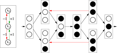
Figure 1: Left: Network with $N=3$ nodes and bias values $a_{0}=a_{2}=0$ and $a_{1}=2$. Right: Dynamics of the network. Transitions between configurations under asynchronous update are indicated by arrows. Under synchronous (parallel) update the system has one unique cyclic attractor only, consisting of the four configurations in the middle row.

non-vanishing couplings $w_{01}=w_{21}=-1$ and $w_{10}=w_{12}=+1$, see Fig. 1. Note that under asynchronous update the sequence of states reached by the dynamics is not unique. The system may branch off to different configurations depending on node update ordering. This is illustrated in Fig. 2(a): Without delay ($\tau=0$) and filter ($\epsilon=1$) the dynamics is irregular, i.e. non-periodic.

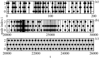
Figure 2: Simulation runs of the three-node network in Fig. 1. (a) Random asynchronous update mode, $\tau=0$, $\epsilon=1$. (b) Filtering $\epsilon=0.01$ but no delay $\tau=0$. (c) Delay $\tau=100$ and no filtering, $\epsilon=1$. A circle plotted at coordinates $(t,i)$ indicates that state $x_{i}$ of node $i$ changes at time $t$.

With filter only ($\tau=0$, $\epsilon=0.01$, Fig. 2(b)), the dynamics is periodic at times, but also intervals of fast irregular flipping occur. Finally, in the presence of delay ($\tau=100$, $\epsilon=1$, Fig. 2(c)) we obtain perfectly ordered dynamics with synchronization of flips. Nodes 0 and 2 change states practically at the same (macro) time, followed by a longer pause until node 1 changes state, etc. With increasing delay time $\tau$ the dynamics under asynchronous update approaches the dynamics under synchronous update (cf. Fig. 1) when viewed on a coarse-grained (macro) time scale.

Let us further quantify the difference between synchronous and asynchronous dynamics. First, a definition of equivalence between the two dynamical modes has to be given. Let us start from the time series ${\bf x}(t)$ of configurations ${\bf x}=(x_{0},\dots,x_{N-1})$ produced by the asynchronous (random serial) update of the model and the respective time series ${\bf y}(u)$ produced by synchronous (parallel) update, using identical initial condition ${\bf y}(0)={\bf x}(0)$. These time series live on different time scales, which we call the micro time scale of single site updates in the asynchronous case, and the macro time scale where each time step is an entire sweep of the system. Assume that at time $t_{u}$ the asynchronous system is in state ${\bf x}(t_{u})={\bf y}(u)$. In order to follow the synchronous update it has to subsequently reach the state ${\bf y}(u+1)$ on a shortest path in phase space. Formally, let us require that there is a micro time $t_{u+1}>t_{u}$ such that ${\bf x}(t_{u+1})={\bf y}(u+1)$ and each node flips at most once in the time interval $[t_{u},t_{u+1}]$. Once this is violated we say that an error has occured at the particular macro time step $u$. This error allows to define a numerical measure of discrepancy between asynchronous and synchronous dynamics. Starting from identical initial conditions, the system is iterated in synchronous and asynchronous modes (here for $u_{\rm total}=10^{7}$ macro time steps). Whenever the resulting time series are no longer equivalent, an error counter is incremented and the system reset to initial condition. The total error $E$ of the run is the number of errors divided by $u_{\rm total}$.

For the network in Fig. 1 and the initial condition $x_{i}=c_{i}=0$ for $i=1,2,3$ the error $E$ is exponentially suppressed with delay time $\tau$ (Fig. 3).

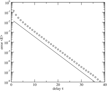
Figure 3: Discrepancy $E$ between the asynchronous and synchronous update mode as a function of the delay time $\tau$ and without filter ($\epsilon=1$). The solid line is the theoretical prediction of the decay $\propto(2/3)^{\tau}$.

The asynchronous dynamics with delay follows the attractor during a time span that increases exponentially with the given delay time. Note that there is only one possibility for the asynchronous dynamics to leave the attractor: When the system is in configuration $(1,1,0)$ or $(0,1,1)$, node $2$ may change state such that the system goes to configuration $(1,0,0)$ or $(0,0,1)$ respectively, whereas the correct next configuration on the attractor is $(0,1,0)$. Consider the case $\epsilon=1$ where $c_{i}=x_{i}$ for all $i$. Let us assume that the system is in configuration $(1,1,1)$ and at time $t_{0}$ node 0 changes state, thereby generating configuration $(0,1,1)$. This decreases the input sum $s_{1}$ below zero such that for $\tau=0$ node $0$ would change state immediately in its next update. With explicit transmission delay $\tau>0$, however, node 1 still “sees” the input sum $s_{i}=0$ generated by the configuration $(1,1,1)$ until time step $t_{0}+\tau$. If node $2$ is chosen for update in this time window $t_{0}+1,\dots,t_{0}+\tau$ it changes state immediately and updates are performed in correct order. The opposite case, that node 2 does not receive an update in any of the $\tau$ time steps, happens with probability $(2/3)^{\tau}$, yielding the correct error decay of the simulation (Fig. 3).

Next we demonstrate that there are cases where also low-pass filtering, $\epsilon\ll 1$, is needed for the asynchronous dynamics to follow the deterministic attractor. Consider a network of $N=5$ nodes with bias values $a_{0}=a_{4}=0$ and $a_{1}=a_{2}=a_{3}=1$. The only non-zero couplings are $w_{10}=w_{21}=w_{31}=w_{42}=+1$ and $w_{01}=w_{43}=-1$. Nodes 0 and 1 form an oscillator, i.e. $(x_{0},x_{1})$ iterate the sequence $(0,0)$, $(1,0)$, $(1,1)$, $(0,1)$. Nodes $2$ and $3$ simply “copy” the state of node $1$ such that under synchronous update always $x_{3}(t)=x_{2}(t)=x_{1}(t-1)$. Consequently, under synchronous update the input sum of node $4$ never changes because the positive contribution from node 2 and the negative contribution from node 3 cancel out. Under asynchronous update, however, the input sum of node 4 may fluctuate because nodes 2 and 3 do not flip precisely at the same time. The effect of the low-pass filter $\epsilon\ll 1$ is to suppress the spreading of such fluctuations on the micro time scale. The influence of the filter is seen in Fig. 4.

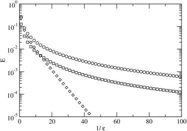
Figure 4: Discrepancy $E$ between the asynchronous and synchronous update mode as a function of the filter parameter $1/\epsilon$ for the network with $N=5$ nodes described in the text. The delay parameter is chosen as $\tau=0$ (circles), $\tau=10$ (squares), and $\tau=1/\epsilon$ (diamonds).

When $\tau$ is kept constant, the error drops algebraically with decreasing $\epsilon$. An exponential decay $E\sim\exp(-\alpha/\epsilon)$ is obtained when $\tau\propto 1/\epsilon$ (the filter can take full effect only in the presence of sufficient delay).

Let us finally consider an example of a larger network with $N=16$ nodes and $L=48$ non-vanishing couplings (chosen randomly from the off-diagonal elements in the matrix $(w_{ij})$ and assigned values $+1$ or $-1$ with probability $1/2$ each; biases are chosen as $a_{i}=\sum_{j}w_{ij}/2$). Simulation runs under pure asynchronous update ($\tau=0$, $\epsilon=1$) typically yield dynamics as in Fig. 5(a).

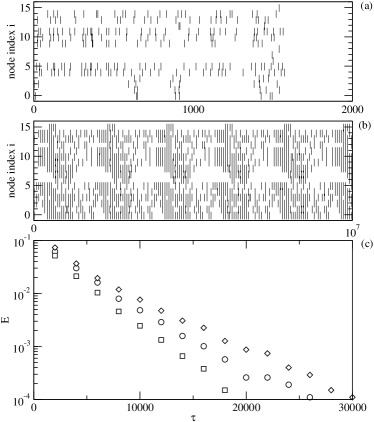
Figure 5: Time series and errors obtained for the network of $N=16$ nodes described in the text. (a) Asynchronous update mode with neither delay nor filtering, $\tau=0$, $\epsilon=1$. A vertical stroke at coordinates $(t,i)$ indicates that node $i$ flips at time $t$. At $t\approx 1600$ the system reaches a fixed point. (b) Same initial condition as in (a), but delay $\tau=50000$ and filtering $\epsilon=1/500$. The system follows a limit cycle of 28 macro time steps. (c) Discrepancy (error $E$) between asynchronous and synchronous update mode as a function of the delay parameter for $\epsilon=50/\tau$ (circles), $\epsilon=40/\tau$ (squares), $\epsilon=25/\tau$ (diamonds).

The time series ${{\bf x}(t)}$ is non-periodic and non-reproducible, i.e. under different order of updates a different series is obtained. For the same initial condition, periodic dynamics is observed in the presence of sufficent transmission delay and filtering, Fig. 5(b). In this case, the system follows precisely the attractor of period 28 found under synchronous update. As seen in Fig. 5(c), the error decays exponentially as a function of the delay time $\tau$.

Let us now turn to the dangers of asynchronous update: There is a fraction of attractors observed under synchronous update that cannot be realized under asynchronous update. Synchronization cannot be sustained if the dynamics is separable. In the trivial case, separability means that the set of nodes can be divided into two subsets that do not interact with each other. Then there is no signal to synchronize one set of nodes with the other and they will go out of phase. In general, synchronization is impossible if the set of flips itself is separable. Consider, as the simplest example, a network of $N=2$ nodes with the couplings $w_{01}=w_{10}=+1$, biases $a_{0}=a_{1}=1$ and the initial condition $(y_{0}(0),y_{1}(0))=(0,1)$. Under synchronous update, the state alternates between vector $(0,1)$ and $(1,0)$. Under asynchronous update with delay time $\tau$, the transition of one node $i$ from $x_{i}=0$ to $x_{i}=1$ causes the other node $j$ to switch from $x_{j}=0$ to $x_{j}=1$ approximately $\tau$ time steps later. The “on”-transitions only trigger subsequent “on”-transitions and, analogously, the “off”-transitions only trigger subsequent “off”-transitions. The dynamics can be divided into two distinct sets of events that do not influence each other. Consequently, synchronization between flips cannot be sustained, as illustrated in Fig. 6.

Figure 6: Dynamics of the network with $N=2$ mutually activating nodes. Rising edges and falling edges desynchronize over time. The two classes of edges form two uncoupled chains of events.

When the phase difference reaches the value $\tau$, on- and off-transitions annihilate. Then the system leaves the attractor and reaches one of the fixed points with $x_{0}=x_{1}$.

These observations have important implications for robust topological motifs in asynchronous networks. First of all, the above example of a small excitatory loop can be quickly generalized to any larger loop with excitatory interactions, as well as to loops with an even number of inhibitory couplings, where in principle similar dynamics could occur. Higher order structures that fail to synchronize include competing modules, e.g. two oscillators (loops with odd number of inhibitory links) that interact with a common target.

In conclusion we find that asynchronously updated networks of autonomous dynamical nodes are able to exhibit a reproducible and quasi-deterministic dynamics under broad conditions if the nodes have transmission delay and low pass filtering as, e.g., observed in regulatory genes. Timing requirements put constraints on the topology of the networks (e.g. suppression of certain loop motifs). With respect to biological gene regulation networks where indeed strong suppression of loop structures is observed Shen-Orr02 ; Milo02 , one may thus speculate about a new constraint on topological motifs of gene regulation: The requirement for deterministic dynamics from asynchronous dynamical networks.

Acknowledgements S.B. thanks D. Chklovskii, M.H. Jensen, S. Maslov, and K. Sneppen for discussions and comments, and the Aspen Center for Physics for hospitality where part of this work has been done.

References

- (1) E. Schrödinger, What is Life? The Physical Aspect of the Living Cell, Cambridge: University Press (1948).
- (2) H. Hirata et al., Science 298, 840 (2002).
- (3) M.B. Elowitz and S. Leibler, Nature 403, 335 (2002).
- (4) A. Hoffmann, A. Levchenko, M.L. Scott, and D. Baltimore, Science 298, 1241-1245 (2002).
- (5) G. Tiana, M.H. Jensen, and K. Sneppen, Eur. Phys. J. B 29, 135-140 (2002).
- (6) P. Smolen, D. A. Baxter, J. H. Byrne, Bull. Math. Biol. 62, 247 (2000).
- (7) N. Rosenfeld, M. B. Elowitz, U. Alon, J. Mol. Biol. 323, 785 (2002).
- (8) M.H. Jensen, K. Sneppen, G. Tiana, FEBS Letters 541, 176-177 (2003).
- (9) S.S. Shen-Orr, R. Milo, S. Mangan, and U. Alon, Nature Genetics 31, 64-68 (2002).
- (10) R. Milo, S. Shen-Orr, S. Itzkovitz, N. Kashtan, D. Chklovskii, and U. Alon, Science 298, 824-827 (2002).