Mixtures of Gaussian process priors

Abstract

Nonparametric Bayesian approaches based on Gaussian processes have recently become popular in the empirical learning community. They encompass many classical methods of statistics, like Radial Basis Functions or various splines, and are technically convenient because Gaussian integrals can be calculated analytically. Restricting to Gaussian processes, however, forbids for example the implemention of genuine nonconcave priors. Mixtures of Gaussian process priors, on the other hand, allow the flexible implementation of complex and situation specific, also nonconcave a priori information. This is essential for tasks with, compared to their complexity, a small number of available training data. The paper concentrates on the formalism for Gaussian regression problems where prior mixture models provide a generalisation of classical quadratic, typically smoothness related, regularisation approaches being more flexible without having a much larger computational complexity.

1 Introduction

The generalisation behaviour of statistical learning algorithms relies essentially on the correctness of the implemented a priori information. While Gaussian processes and the related regularisation approaches have, on one hand, the very important advantage of being able to formulate a priori information explicitly in terms of the function of interest (mainly in the form of smoothness priors which have a long tradition in density estimation and regression problems [18, 17, 5]) they implement, on the other hand, only simple concave prior densities corresponding to quadratic errors. Especially complex tasks would require typically more general prior densities. Choosing mixtures of Gaussian process priors combines the advantage of an explicit formulation of priors with the possibility of constructing general non-concave prior densities.

While mixtures of Gaussian processes are technically a relatively straightforward extension of Gaussian processes, which turns out to be a computational advantage, practically they are much more flexible and are able to produce in principle, i.e., in the limit of infinite number of components, any arbitrary prior density.

As example, consider an image completion task, where an image have to be completed, given a subset of pixels (‘training data’). Simply requiring smoothness of grey level values would obviously not be sufficient if we expect, say, the image of a face. In that case the prior density should reflect that a face has specific constituents (e.g., eyes, mouth, nose) and relations (e.g., typical distances between eyes) which may appear in various variations (scaled, translated, deformed, varying lightening conditions).

While ways how prior mixtures can be used in such situations have already been outlined in [6, 7, 8, 9, 10] this paper concentrates on the general formalism and technical aspects of mixture models and aims in showing their computational feasibility. Sections 2–4 provide the necessary formulae while Section 5 exemplifies the approach for an image completion task.

Finally, we remark that mixtures of Gaussian process priors do usually not result in a (finite) mixture of Gaussians [3] for the function of interest. Indeed, in density estimation, for example, arbitrary densities not restricted to a (finite) mixture of Gaussians can be produced by a mixture of Gaussian prior processes.

2 The Bayesian model

Let us consider the following random variables:

• $x$, representing (a vector of) independent, visible variables (‘measurement situations’),

• $y$, being (a vector of) dependent, visible variables (‘measurement results’), and

• $h$, being the hidden variables (‘possible states of Nature’).

A Bayesian approach is based on two model inputs [1, 11, 4, 12]:

• A likelihood model $p(y|x,h)$, describing the density of observing $y$ given $x$ and $h$. Regarded as function of $h$, for fixed $y$ and $x$, the density $p(y|x,h)$ is also known as the ($x$–conditional) likelihood of $h$.

• A prior model $p(h|D_{0})$, specifying the a priori density of $h$ given some a priori information denoted by $D_{0}$ (but before training data $D_{T}$ have been taken into account).

Furthermore, to decompose a possibly complicated prior density into simpler components, we introduce continuous hyperparameters $\theta$ and discrete hyperparameters $j$ (extending the set of hidden variables to $\tilde{h}$ = $(h,\theta,j)$),

$$p(h|D_{0})=\int\!d\theta\sum_{j}p(h,\theta,j|D_{0}).$$ (1)

In the following, the summation over $j$ will be treated exactly, while the $\theta$–integral will be approximated. A Bayesian approach aims in calculating the predictive density for outcomes $y$ in test situations $x$

$$p(y|x,D)=\int\!dh\,p(y|x,h)\,p(h|D),$$ (2)

given data $D$ = $\{D_{T},D_{0}\}$ consisting of a priori data $D_{0}$ and i.i.d. training data $D_{T}$ = $\{(x_{i},y_{i})|1\leq i\leq n\}$. The vector of all $x_{i}$ ($y_{i}$) will be denoted $x_{T}$ $(y_{T})$. Fig.1 shows a graphical representation of the considered probabilistic model.

In saddle point approximation (maximum a posteriori approximation) the $h$–integral becomes

$$p(y|x,D)\approx p(y|x,h^{*}),$$ (3)

$$h^{*}=\,{\rm argmax}_{h\in{\cal H}}p(h|D),$$ (4)

assuming $p(y|x,h)$ to be slowly varying at the stationary point. The posterior density is related to ($x_{T}$–conditional) likelihood and prior according to Bayes’ theorem

$$p(h|D)=\frac{p(y_{T}|x_{T},h)\,p(h|D_{0})}{p(y_{T}|x_{T},D_{0})},$$ (5)

where the $h$–independent denominator (evidence) can be skipped when maximising with respect to $h$. Treating the $\theta$–integral within $p(h|D)$ also in saddle point approximation the posterior must be maximised with respect to $h$ and $\theta$ simultaneously .

Figure 1: Graphical representation of the considered probabilistic model, factorising according to $p(x_{T},y_{T},x,y,h,\theta,j,(\beta)|D)$ = $p(x_{T})$ $p(x)$ $p(y_{T}|x_{T},h,(\beta))$ $p(y|x,h,(\beta))$ $p(h|\theta,j,D_{0},(\beta))$ $p(\theta,j,(\beta)|D_{0})$. (The variable $\beta$ is introduced in Section 3.) Circles indicate visible variables.

3 Gaussian regression

In general density estimation problems $p(y_{i}|x_{i},h)$ is not restricted to a special form, provided it is non–negative and normalised [9, 10]. In this paper we concentrate on Gaussian regression where the single data likelihoods are assumed to be Gaussians

$$p(y_{i}|x_{i},h)=\sqrt{\frac{\beta}{2\pi}}e^{-\frac{\beta}{2}(h(x_{i})-y_{i})^{2}}.$$ (6)

In that case the unknown regression function $h(x)$ represents the hidden variables and $h$–integration means functional integration $\int dh\rightarrow\int\prod_{x}dh(x)$.

As simple building blocks for mixture priors we choose Gaussian (process) prior components [2, 17, 14],

$$p(h|\beta,\theta,j,D_{0})=\left(\frac{\beta}{2\pi}\right)^{\frac{d}{2}}\left(\det{\bf K}_{j}(\theta)\right)^{\frac{1}{2}}$$

$$\times e^{-\frac{\beta}{2}\mbox{$\left(h-t_{j}(\theta),\,{\bf K}_{j}(\theta)(h-t_{j}(\theta))\right)$}}$$ (7)

the scalar product notation $\left(\cdot,\,\cdot\right)$ standing for $x$–integration. The mean $t_{j}(\theta)(x)$ will in the following also be called an (adaptive) template function. Covariances ${\bf K}^{-1}_{j}/\beta$ are real, symmetric, positive (semi–)definite (for positive semidefinite covariances the null space has to be projected out). The dimension $d$ of the $h$–integral becomes infinite for an infinite number of $x$–values (e.g. continuous $x$). The infinite factors appearing thus in numerator and denominator of (5) however cancel. Common smoothness priors have $t_{j}(\theta)=0$ and as ${\bf K}_{j}$ a differential operator, e.g., the negative Laplacian.

Analogously to simulated annealing it will appear to be very useful to vary the ‘inverse temperature’ $\beta$ simultaneously in (6) (for training but not necessarily for test data) and (7). Treating $\beta$ not as a fixed variable, but including it explicitly as hidden variable, the formulae of Sect. 2 remain valid, provided the replacement $h\rightarrow(h,\beta)$ is made, e.g. $p(y_{i}|x_{i},h)\rightarrow p(y_{i}|x_{i},h,\beta)$ (see also Fig.1).

Typically, inverse prior covariances can be related to approximate symmetries. For example, assume we expect the regression function to be approximately invariant under a permutation of its arguments $h(x)\approx h(\sigma(x))$ with $\sigma$ denoting a permutation. Defining an operator ${\bf S}$ acting on $h$ according to ${\bf S}h(x)=h(\sigma(x))$, we can define a prior process with inverse covariance

$${\bf K}=({\bf I}-{\bf S})^{T}({\bf I}-{\bf S}),$$ (8)

with identity ${\bf I}$ and the superscript ^T denoting the transpose of an operator. The corresponding prior energy

$$E_{0}=\frac{1}{2}\left(h,\,{\bf K}\,h\right)=\frac{1}{2}\Big{(}(h-{\bf S})h,\,(h-{\bf S})h\Big{)},$$ (9)

is a measure of the deviation of $h$ from an exact symmetry under ${\bf S}$. Similarly, we can consider a Lie group ${\bf S}$ = $e^{\theta{\bf s}}$ with ${\bf s}$ being the generator of the infinitesimal symmetry transformation. In that case a covariance

$${\bf K}=\frac{1}{\theta^{2}}({\bf I}-{\bf S}_{\rm inf})^{T}({\bf I}-{\bf S}_{\rm inf})={\bf s}^{T}{\bf s},$$ (10)

with prior energy

$$E_{0}=\frac{1}{2}\left({\bf s}h,\,{\bf s}h\right),$$ (11)

can be used to implement approximate invariance under the infinitesimal symmetry transformation ${\bf S}_{\rm inf}$ = ${\bf I}+\theta{\bf s}$. For appropriate boundary conditions, a negative Laplacian ${\bf K}$ can thus be interpreted as enforcing approximate invariance under infinitesimal translations, i.e., for ${\bf s}$ = $\partial/\partial x$.

4 Prior mixtures

4.1 General formalism

Decomposed into components the posterior density becomes

$$p(h,\beta|D) \!\propto\! \!\int\!d\theta\,\sum_{j}^{m}p(y_{T}|x_{T},h,\beta)$$

$$\!\!\!\!\!\!\times\;p(h|\beta,\theta,j,D_{0})\,p(\beta,\theta,j|D_{0}).$$

Writing probabilities in terms of energies, including parameter dependent normalisation factors and skipping parameter independent factors yields

$$p(y_{T}|x_{T},h,\beta) \propto e^{-\beta E_{T}+\frac{n}{2}\ln\beta}$$

$$p(h|\beta,\theta,j,D_{0}) = e^{-\beta E_{0,j}+\frac{d}{2}\ln\beta}$$

$$\times e^{\frac{1}{2}\ln\det{\bf K}_{j}(\theta)}$$

$$p(\beta,\theta,j|D_{0}) \propto e^{-E_{\theta,\beta,j}}.$$

This defines hyperprior energies $E_{\theta,\beta,j}$, prior energies $E_{0,j}$ (‘quadratic concepts’)

$$E_{0,j}=\frac{1}{2}\mbox{$\Big{(}h-t_{j}(\theta),\,{\bf K}_{j}(\theta)(h-t_{j}(\theta,j))\Big{)}$},$$ (14)

(the generalisation to a sum of quadratic terms $E_{0,j}=\sum_{k}E_{0,k,j}$ is straightforward) and training or likelihood energy (training error)

$$E_{T}=\frac{1}{2}\sum_{i}^{n}(h(x_{i})-y_{i})^{2}$$ (15)

$$=\frac{1}{2}\left(\mbox{$\Big{(}h-t_{T},\,{\bf K_{T}}(h-t_{T})\Big{)}$}+\sum_{i}^{n}V_{T}(x_{i})\right).$$

The second line is a ‘bias–variance’ decomposition where

$$t_{T}(x_{i})=\sum_{k}^{n_{x_{i}}}\frac{y_{k}(x)}{n_{x_{i}}},$$ (16)

is the mean of the $n_{x_{i}}$ training data available for $x_{i}$, and

$$V_{T}(x_{i})=\sum_{k}^{n_{x_{i}}}\frac{y^{2}_{k}(x)}{n_{x_{i}}}-t_{T}^{2}(x_{i}),$$ (17)

is the variance of $y_{i}$ values at $x_{i}$. ($V_{i}$ vanishes if every $x_{i}$ appears only once.) The diagonal matrix ${\bf K}_{T}$ is restricted to the space of $x$ for which training data are available and has matrix elements $n_{x}$.

4.2 Maximum a posteriori approximation

In general density estimation the predictive density can only be calculated approximately, e.g. in maximum a posteriori approximation or by Monte Carlo methods. For Gaussian regression, however the predictive density of mixture models can be calculated exactly for given $\theta$ (and $\beta$). This provides us with the opportunity to compare the simultaneous maximum posterior approximation with respect to $h$ and $\theta$ with an analytical $h$–integration followed by a maximum posterior approximation with respect to $\theta$.

Maximising the posterior (with respect to $h$, $\theta$, and possibly $\beta$) is equivalent to minimising the mixture energy (regularised error functional [13, 17, 15, 16])

$$E=-\ln\sum_{j}^{m}e^{-E_{j}+c_{j}},$$ (18)

with component energies

$$E_{j}=\beta E_{h,j}+E_{\theta,\beta,j},\quad E_{h,j}=E_{T}+E_{0,j},$$ (19)

and

$$c_{j}(\theta,\beta)=\frac{1}{2}\ln\det{\bf K}_{j}(\theta)+\frac{d+n}{2}\ln\beta.$$ (20)

In a direct saddle point approximation with respect to $h$ and $\theta$ stationarity equations are obtained by setting the (functional) derivatives with respect to $h$ and $\theta$ to zero,

$$0\!\!\! = \!\!\!\!\sum_{j}^{m}\!a_{j}\Big{(}{\bf K}_{T}(h-t_{T})+\!{\bf K}_{j}(h-t_{j})\Big{)},\;\;\;\;\;\;\;$$ (21)

$$0\!\!\! = \!\!\!\!\sum_{j}^{m}a_{j}\Bigg{(}\frac{\partial E_{j}}{\partial\theta}-{\rm Tr}\,\left({\bf K}_{j}^{-1}\frac{\partial{\bf K}_{j}}{\partial\theta}\right)\Bigg{)},$$ (22)

where the derivatives with respect to $\theta$ are matrices if $\theta$ is a vector,

$$a_{j} = p(j|h,\theta,D_{0})$$

$$= \frac{e^{-\beta E_{0,j}-E_{\theta,\beta,j}+\frac{1}{2}\ln\det{\bf K}_{j}}}{\sum_{k}^{m}e^{-\beta E_{0,k}-E_{\theta,\beta,k}+\frac{1}{2}\ln\det{\bf K}_{k}}},$$

and

$$\frac{\partial E_{j}}{\partial\theta} = \frac{\partial E_{\theta,\beta,j}}{\partial\theta}+\beta\left(\frac{\partial t_{j}}{\partial\theta},\;{\bf K}_{j}(t_{j}-h)\right)\$$ (24)

$$\!\!\!+\frac{\beta}{2}\Big{(}(h-t_{j}),\,\frac{\partial{\bf K}_{j}}{\partial\theta}(h-t_{j})\Big{)}.$$

Eq.(21) can be rewritten

$$h={\bf K}_{a}^{-1}\left({\bf K}_{T}t_{T}+\sum_{l}^{m}a_{j}{\bf K}_{j}t_{j}\right),$$ (25)

with

$${\bf K}_{a}=\left({\bf K}_{T}+\sum_{j}^{m}a_{j}{\bf K}_{j}\right).$$ (26)

Due to the presence of $h$–dependent factors $a_{j}$, Eq.(25) is still a nonlinear equation for $h(x)$. For the sake of simplicity we assumed a fixed $\beta$; it is no problem however to solve (21) and (22) simultaneously with an analogous stationarity equation for $\beta$.

4.3 Analytical solution

The optimal regression function under squared–error loss — for Gaussian regression identical to the log–loss of density estimation — is the predictive mean. For mixture model (4.1) one finds, say for fixed $\beta$,

$$\bar{y}=\int\!dy\,y\,p(y|x,D)=\sum_{j}\int\!d\theta\;b_{j}(\theta)\,\bar{t}_{j}(\theta),$$ (27)

with mixture coefficients

$$b_{j}(\theta) = p(\theta,j|D)$$

$$= \frac{p(\theta,j)\,p(y_{T}|x_{T},D_{0},\theta,j)}{\sum_{j}\int\!d\theta p(\theta,j)\,p(y_{T}|x_{T},D_{0},\theta,j)}.$$

The component means $\bar{t}_{j}$ and the likelihood of $\theta$ can be calculated analytically [17, 14]

$$\bar{t}_{j} = \left({\bf K}_{T}+{\bf K}_{j}\right)^{-1}\left({\bf K}_{T}t_{T}+{\bf K}_{j}t_{j}\right)$$ (29)

$$= t_{j}+{\bf K}_{j}^{-1}\widetilde{\bf K}_{j}(t_{T}-t_{j}),$$

and

$$p(y_{T}|x_{T},D_{0},\theta,j)=e^{-\beta\widetilde{E}_{0,j}+\frac{1}{2}\ln\det(\frac{\beta}{2\pi}\widetilde{\bf K}_{j})},$$ (30)

where

$$\widetilde{E}_{0,j}(\theta) = \frac{1}{2}\big{(}t_{T}-t_{j},\,\widetilde{\bf K}_{j}(t_{T}-t_{j})\big{)},\quad$$ (31)

$$\widetilde{\bf K}_{j}(\theta) = ({\bf K}_{T}^{-1}+{\bf K}_{j,TT}^{-1})^{-1},$$ (32)

and ${\bf K}_{j,TT}^{-1}$ is the projection of the covariance ${\bf K}_{j}^{-1}$ into the $\tilde{n}$–dimensional space for which training data are available. ($\tilde{n}\leq n$ is the number of data with distinct $x$–values.)

The stationarity equation for a maximum a posteriori approximation with respect to $\theta$ is at this stage found from (4.3,30)

$$0=\sum_{j}b_{j}\left(\frac{\partial\widetilde{E}_{j}}{\partial\theta}-{\rm Tr}\left(\widetilde{\bf K}_{j}^{-1}\frac{\partial\widetilde{\bf K}_{j}}{\partial\theta}\right)\right),$$ (33)

where $\widetilde{E}_{j}$ = $\beta\widetilde{E}_{0,j}$ + $E_{\theta,\beta,j}$. Notice that Eq.(33) differs from Eq.(22) and requires only to deal with the $\tilde{n}\times\tilde{n}$–matrix $\widetilde{\bf K}$. The coefficient $b^{*}_{j}$ = $b_{j}(\theta^{*})$ for $\theta$ set to its maximum posterior value is of form (4.2) with the replacements ${\bf K}_{j}\rightarrow\widetilde{\bf K}_{j}$, $E_{j}\rightarrow\widetilde{E}_{j}$.

4.4 High and low temperature limits

Low and high temperature limits are extremely useful because in both cases the stationarity Eq.(21) becomes linear, corresponding thus to classical quadratic regularisation approaches.

In the high temperature limit $\beta\rightarrow 0$ the exponential factors $a_{j}$ become $h$–independent

$$a_{j}\stackrel{{\scriptstyle\beta\rightarrow 0}}{{\longrightarrow}}a^{0}_{j}=\frac{e^{-E_{\theta,\beta,j}+\frac{1}{2}\ln\det{\bf K}_{j}}}{\sum_{k}^{m}e^{-E_{\theta,\beta,k}+\frac{1}{2}\ln\det{\bf K}_{k}}},$$ (34)

(for $b_{j}^{*}\rightarrow b_{j}^{0,*}$ replace ${\bf K}_{j}$ by $\widetilde{\bf K}_{j}$). The solution $h=\bar{t}$ is a (generalised) ‘complete template average’

$$\bar{t}={\bf K}_{a^{0}}^{-1}\left({\bf K_{T}}t_{T}+\sum_{l}^{m}a^{0}_{j}\,{\bf K}_{j}t_{j}\right),$$ (35)

with

$${\bf K}_{a^{0}}={\bf K}_{T}+\sum_{j}a_{j}^{0}\,{\bf K}_{j}.$$ (36)

This high temperature solution corresponds to the minimum of the quadratic functional $E_{T}+\sum_{j}^{m}a_{j}^{0}E_{h,j}$,

In the low temperature limit $\beta\rightarrow\infty$ only the maximal component contributes, i.e.,

$$a_{j}\stackrel{{\scriptstyle\beta\rightarrow\infty}}{{\longrightarrow}}a^{\infty}_{j}=\left\{\begin{array}[]{r@{\quad: \quad}l}1&j={\rm argmin}_{j}E_{h,j}\\ 0&j\neq{\rm argmin}_{j}E_{h,j}\end{array}\right.,$$ (37)

(for $b_{j}^{*}$ replace $E_{h,j}$ by $\widetilde{E}_{j}$) assuming $E_{\beta,\theta,j}$ = $E_{\beta}$ + $E_{\theta,j}$ or $E_{\beta,\theta,j}$ = $E_{\beta}$ + $E_{j}$ +$\beta E_{\theta}$. Hence, low temperature solutions $h=\bar{t}_{j}$, are all (generalised) ‘component averages’ $\bar{t}_{j}$ provided they fulfil the stability condition

$$E_{h,j}(h=\bar{t}_{j})<E_{h,j^{\prime}}(h=\bar{t}_{j}),\quad\forall j^{\prime}\neq j,$$ (38)

or, after performing a (generalised) ‘bias–variance’ decomposition, $2V_{j}<{B}_{j^{\prime}}(j,j)+2V_{j^{\prime}}$, with $m\times m$ matrices

$${B}_{j}(k,l)=\Big{(}\bar{t}_{k}-\bar{t}_{j},\,\left({\bf K}_{D}+{\bf K}_{j}\right)\,(\bar{t}_{l}-\bar{t}_{j})\Big{)}$$ (39)

and (generalised) ‘template variances’

$$V_{j}\!\! \!\!= \frac{1}{2}\Bigg{(}\Big{(}t_{T},\,{\bf K}_{T}\,t_{T}\Big{)}+\Big{(}t_{j},\,{\bf K}_{j}\,t_{j}\Big{)}\quad$$ (40)

$$- \Big{(}\bar{t}_{j},({\bf K}_{T}+{\bf K}_{j})\,\bar{t}_{j}\Big{)}\Bigg{)}=\widetilde{E}_{0,j}.$$

That means single component averages $\bar{t}_{j}$ (which minimise $E_{h,j}$ and thus $-\beta E_{j}+c_{j}$) become solutions at zero temperature $1/\beta$ in case their (generalised) variance $V_{j}$ measuring the discrepancy between data and prior term is small enough.

4.5 Equal covariances

Especially interesting are $j$–independent ${\bf K}_{j}(\theta)$ = ${\bf K}_{0}(\theta)$ with $\theta$–independent determinants so $\det{\bf K}_{j}$ or $\det\widetilde{\bf K}_{j}$, respectively, do not have to be calculated.

Notice that this still allows completely arbitrary parameterisations of $t_{j}(\theta)$. Thus, the template function can for example be a parameterised model, e.g., a neural network or decision tree, and maximising the posterior with respect to $\theta$ corresponds to training that model. In such cases the prior term forces the maximum posterior solution $h$ to be similar (as defined by ${\bf K_{0}}$) to this trained parameterised reference model.

The condition of invariant $\det{\bf K}_{0}(\theta)$ does not exclude adaption of covariances. For example, transformations for real, symmetric positive definite ${\bf K}_{0}(\theta)$ leaving determinant and eigenvalues (but not eigenvectors) invariant are of the form ${\bf K}(\theta_{0})\rightarrow{\bf K}(\theta)={\bf O}(\theta){\bf K}{\bf O}^{-1}(\theta)$ with real, orthogonal ${\bf O}^{-1}$ = ${\bf O}^{T}$. This allows for example to adapt the sensible directions of multidimensional Gaussians. A second kind of transformations changing eigenvalues but not eigenvectors and determinant is of the form ${\bf K}(\theta_{0})={\bf O}{\bf D}(\theta_{0}){\bf O}^{T}$ $\rightarrow{\bf K}(\theta)={\bf O}{\bf D}(\theta){\bf O}^{T}$ if the product of eigenvalues of the real, diagonal ${\bf D}(\theta_{0})$ and ${\bf D}(\theta)$ are equal.

Eqs.(29,35) show that the high temperature solution becomes a linear combination of the (potential) low temperature solutions

$$\bar{t}=\sum_{j}^{m}a^{0}_{j}\bar{t}_{j}=\sum_{j}^{m}b^{0,*}_{j}\bar{t}_{j}.$$ (41)

Similarly, Eq.(21) simplifies to

$$h=\sum_{j}^{m}a_{j}\bar{t}_{j}=\bar{t}+\sum_{j}^{m}(a_{j}-a_{j}^{0})\,\bar{t}_{j},$$ (42)

and Eq.(4.2) to

$$a_{j}=\frac{e^{-\frac{\beta}{2}a{B}_{j}a-\widetilde{E}_{j}}}{\sum_{k}e^{-\frac{\beta}{2}a{B}_{k}a-\widetilde{E}_{k}}}=\frac{b_{j}\,e^{-\frac{\beta}{2}a{B}_{j}a}}{\sum_{k}b_{k}\,e^{-\frac{\beta}{2}a{B}_{k}a}},$$ (43)

introducing vector $a$ with components $a_{j}$, $m\times m$ matrices $B_{j}$ defined in (39). Eq.(42) is still a nonlinear equation for $h$, it shows however that the solutions must be convex combinations of the $h$–independent $\bar{t}_{j}$ (see Fig. 2). Thus, it is sufficient to solve Eq.(43) for $m$ mixture coefficients $a_{j}$ instead of Eq.(21) for the function $h$.

Figure 2: Left: Example of a solution space for $m$ = 3. Shown are three low temperature solutions $\bar{t}_{j}$, high temperature solution $\bar{t}$, and a possible solution $h$ at finite $\beta$. Right: Exact $b_{1}$ vs. (dominant) $a_{1}$ (dashed) for $m$ = $2$, $b$ = 2, $\widetilde{E}_{1}$ = 0.405, $\widetilde{E}_{2}$ = 0.605.

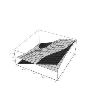
Figure 3: Shown are the plots of $f_{1}(a_{1})=a_{1}$ and $f_{2}(a_{1})=\frac{1}{2}\left(\tanh\Delta+1\right)$ within the inverse temperature range $0\leq\beta\leq 4$ (for $b=2$, $\widetilde{E}_{2}-\widetilde{E}_{1}$ = $0.1\beta$). Notice the appearance of a second stable solution at low temperatures.

For two prior components, i.e., $m=2$, Eq.(42) becomes

$$h=\frac{\bar{t}_{1}+\bar{t}_{2}}{2}+\left(\tanh\Delta\right)\frac{\bar{t}_{1}-\bar{t}_{2}}{2},$$ (44)

with

$$\Delta=\frac{E_{2}-E_{1}}{2}=\frac{\beta}{4}\,b(2a_{1}-1)+\frac{\widetilde{E}_{2}-\widetilde{E}_{1}}{2},$$ (45)

because the matrices $B_{j}$ are in this case zero except $B_{1}(2,2)=B_{2}(1,1)=b$. For $E_{\theta,\beta,j}$ uniform in $j$ we have $(\bar{t}_{1}+\bar{t}_{2})/2$ = $\bar{t}$ so that $a_{j}^{0}$ = $0.5$. The stationarity Eq.(43), being analogous to the celebrated mean field equation of a ferromagnet, can be solved graphically (see Fig.3 and Fig.2 for a comparison with $b_{j}$), the solution is given by the point where

$$a_{1}=\frac{1}{2}\left(\tanh\Delta+1\right).$$ (46)

5 A numerical example

As numerical example we study a two component mixture model for image completion. Assume we expect an only partially known image (corresponding to pixel-wise training data drawn with Gaussian noise from the original image) to be similar to one of the two template images shown in Fig.4. Next, we include hyperparameters parameterising deformations of templates. In particular, we have chosen translations ($\theta_{1}$, $\theta_{2}$) a scaling factor $\theta_{3}$, and a rotation angle (around template center) $\theta_{4}$.

Interestingly, it turned out that due to the large number of data ($\tilde{n}\approx$ 1000) it was easier to solve Eq.(21) for the full discretized image than to invert (32) in the space of training data. A prior operator ${\bf K}_{0}$ has been implemented as a $3\times 3$ negative Laplacian filter. (Notice that using a Laplacian kernel, or another smoothness measure, instead of a straight template matching using simply the squared error between image and template, leads to a smooth interpolation between data and templates.) Completed images $h$ for different $\beta$ have been found by iterating according to

$$h^{k+1}=h^{k}+\eta{\bf A}^{-1}\Big{[}{\bf K}_{T}(t_{T}-h^{k})+{\bf K}_{0}\Big{(}\sum_{j}a_{j}^{k}t_{j}-h^{k}\Big{)}\Big{]},$$ (47)

performed alternating with $\theta$–minimisation. A Gaussian learning matrix ${\bf A}^{-1}$ (implemented by a $5\times 5$ binomial filter) proved to be successful. Typically, the relaxation factor $\eta$ has been set to $0.05$.

Being a mixture model with $m=2$ the situation is that of Fig.3. Typical solutions for large and small $\beta$ are shown in Fig.4.

Figure 4: Top row, from left to right: Data points sampled with Gaussian noise, two template functions $t_{1}$, $t_{2}$. Bottom row, from left to right: Original, reconstructed solutions (regression function $h$, 180$\times$240 pixels) at low and at high temperature.

6 Conclusions

Prior mixture models are capable to build complex prior densities from simple, e.g., Gaussian components. Going beyond classical quadratic regularisation approaches, they still can use the nice analytical features of Gaussians, and allow to control the degree of the resulting non-convexity explicitly. Combined with parameterised component mean functions and covariances they seem to provide a powerful tool.

Acknowledgements The author was supported by a Postdoctoral Fellowship (Le 1014/1–1) from the Deutsche Forschungsgemeinschaft and a NSF/CISE Postdoctoral Fellowship at the Massachusetts Institute of Technology. Part of the work was done during the seminar ‘Statistical Physics of Neural Networks’ at the Max–Planck–Institut für Physik komplexer Systeme, Dresden. The author also wants to thank Federico Girosi, Tomaso Poggio, Jörg Uhlig, and Achim Weiguny for discussions.

References

- [1] Berger, J.O.: Statistical Decision Theory and Bayesian Analysis. New York: Springer Verlag, 1980.
- [2] Doob, J.L.: Stochastic Processes. New York: Wiley, 1953 (New edition 1990).
- [3] Everitt, B.S. & Hand, D.J.: Finite Mixture Distributions. Chapman & Hall, 1981.
- [4] Gelman A., Carlin, J.B., Stern, H.S., & Rubin, D.B.: Bayesian Data Analysis. New York: Chapman & Hall, 1995.
- [5] Girosi, F., Jones, M., & Poggio, T.: Regularization Theory and Neural Networks Architectures. Neural Computation 7 (2), 219–269, 1995.
- [6] Lemm, J.C.: Prior Information and Generalized Questions. A.I.Memo No. 1598, C.B.C.L. Paper No. 141, Massachusetts Institute of Technology, 1996. (available at http://pauli.uni–muenster.de/∼lemm)
- [7] Lemm, J.C.: How to Implement A Priori Information: A Statistical Mechanics Approach. Technical Report MS-TP1-98-12, Universität Münster, 1998. (cond-mat/9808039, also available at http://pauli.uni–muenster.de/∼lemm.)
- [8] Lemm, J.C.: Quadratic Concepts. In Niklasson, L, Boden, M, Ziemke, T.(eds.): Proceedings of the 8th International Conference on Artificial Neural Networks (ICANN 98), Skövde, Sweden, September 2-4, 1998, Springer Verlag, 1998.
- [9] Lemm, J.C.: Bayesian Field Theory. Technical Report MS-TP1-99-1, Universität Münster, 1999. (available at http://pauli.uni–muenster.de/∼lemm.)
- [10] Lemm, J.C., Uhlig, J., & Weiguny, A.: A Bayesian Approach to Inverse Quantum Statistics. Technical Report MS-TP1-99-6, Universität Münster, 1999. (cond-mat/9907013, also available at http://pauli.uni–muenster.de/∼lemm.)
- [11] Robert, C.P.: The Bayesian Choice. New York: Springer Verlag, 1994.
- [12] Sivia, D.S.: Data Analysis: A Bayesian Tutorial. Oxford: Oxford University Press, 1996.
- [13] Tikhonov A.N. & Arsenin V.: Solution of Ill–posed Problems. New York: Wiley, 1977.
- [14] Williams, C.K.I. & Rasmussen, C.E.: Gaussian processes for regression. In Proc. NIPS8, MIT Press, 1996.
- [15] Vapnik, V.N.: Estimation of dependencies based on empirical data. New York: Springer Verlag, 1982.
- [16] Vapnik, V.N.: Statistical Learning Theory. New York: Wiley, 1998.
- [17] Wahba, G.: Spline Models for Observational Data. Philadelphia: SIAM, 1990.
- [18] Whittaker, E.T., On a new method of graduation. Proc. Edinborough Math. Assoc., 78, 81-89, 1923.