On the Viscosity of Emulsions

Abstract

Combining direct computations with invariance arguments, Taylor’s constitutive equation for an emulsion can be extrapolated to high shear rates. We show that the resulting expression is consistent with the rigorous limits of small drop deformation and that it bears a strong similarity to an a priori unrelated rheological quantity, namely the dynamic (frequency dependent) linear shear response. More precisely, within a large parameter region the nonlinear steady–state shear viscosity is obtained from the real part of the complex dynamic viscosity, while the first normal stress difference is obtained from its imaginary part. Our experiments with a droplet phase of a binary polymer solution (alginate/caseinate) can be interpreted by an emulsion analogy. They indicate that the predicted similarity rule generalizes to the case of moderately viscoelastic constituents that obey the Cox–Merz rule.

1 Introduction

Apart from their technological importance, emulsions have served as model systems accessible to rigorous theoretical modeling. The study of emulsions consisting of droplets of a liquid dispersed in another liquid has thus contributed substantially to our understanding of the rheology of complex fluids. However, although major theoretical achievements date back to the beginning of the $20^{\rm th}$ century, further progress turned out to be difficult. The macroscopic rheological properties of emulsions are determined by the reaction of the individual drops to the flow field, which in turn is modified by the presence of other drops. The mutual hydrodynamic interactions of drops complicates substantially the mathematical description. Moreover, depending on system parameters and flow type, droplets may break under steady flow conditions if a certain critical strain rate is exceeded. Rigorous calculations of the constitutive equation have therefore concentrated on very dilute emulsions and on conditions where drops are only weakly deformed. Sometimes, however, it is desirable to have an approximate expression, which — though not rigorous — can serve for practical purposes as a quantitative description in the parameter region beyond the ideal limits. As far as the dependence of the viscoelastic properties of an emulsion on the volume fraction $\phi$ of the dispersed phase is concerned, such an approximation has been given by Oldroyd (1953). It is not rigorous beyond first order in $\phi$ but serves well some practical purposes even at rather high volume fractions. It seems not reasonable to look for a comparably simple approximation for the dependence of shear viscosity $\eta$ on shear rate $\dot{\gamma}$ that covers the whole range of parameters, where all kinds of difficult break–up scenarios are known to occur. In the next section, we propose instead a less predictive expression which contains an average drop size $R$ (that may change with shear rate) as a phenomenological parameter. The latter has to be determined independently either from theory or experiment. It turns out, however, that for a substantial range of viscosity ratios and shear rates, the expression for $\eta(\dot{\gamma})$ is to a large extent independent of morphology. For conditions, where drops do not break outside this region, we point out a similarity relation between this expression and the frequency dependent viscoelastic moduli $G^{\prime}(\omega)$, $G^{\prime\prime}(\omega)$, similar to the Cox–Merz rule in polymer physics. More precisely, we show that in the limit of small drop deformation, the constitutive equation of an emulsion composed of Newtonian constituents of equal density can be obtained from the frequency dependent linear response to leading order in capillary number ${\cal C}$ and (reciprocal) viscosity ratio $\lambda^{-1}$. And we argue that the identification is likely to represent a good approximation beyond this limit in a larger part of the ${\cal C}-\lambda$ parameter plane. Experimentally, this similarity relation can be tested directly, without interference of theoretical modeling, by comparing two independent sets of rheological data. In summary, our theoretical discussion provokes two major empirical questions. (1) If drops break: does the expression for the viscosity derived in Eq.(18) describe the data with $R$ the average drop size at a given shear rate? (2) If drops do not break below a certain characteristic capillary number $C^{*}(\lambda)$: does the proposed similarity rule hold? To what extent does it generalize to non–Newtonian constituents? In Section 3 we address mainly the second question by experiments with a quasi–static droplet phase of a mixture of moderately viscoelastic polymer solutions.

2 Theory

2.1 Taylor’s constitutive equation for emulsions

A common way to characterize the rheological properties of complex fluids such as emulsions, suspensions, and polymer solutions, is by means of a constitutive equation or an equation of state that relates the components $p_{ij}+p\delta_{ij}$ of the stress tensor to the rate–of–strain tensor $e_{ij}$. This relation can account for all the internal heterogeneity and the complexity and interactions of the constituents if only the system may be represented as a homogeneous fluid on macroscopic scales. The form of possible constitutive equations is restricted by general symmetry arguments, which provide guidelines for the construction of phenomenological expressions Oldroyd (1950, 1958). On the other hand, for special model systems the constitutive equations may be calculated directly at least for some restricted range of parameters. An early example for a direct computation of the constitutive equation of a complex fluid is Einstein’s formula

$$\eta=\eta_{c}\left(1+\frac{5}{2}\phi\right)$$ (1)

for the shear viscosity $\eta\equiv p_{12}/e_{12}$ of a dilute suspension (particle volume fraction $\phi\ll 1$). It is obtained by solving Stokes’ equation for an infinite homogeneous fluid of viscosity $\eta_{c}$ containing a single solid sphere. For a sufficiently dilute suspension, the contributions of different particles to the overall viscosity $\eta$ can be added independently, giving an effect proportional to $\phi$. In close analogy Taylor (1932) calculated $\eta$ for a steadily sheared dilute suspension of droplets of an incompressible liquid of viscosity $\eta_{d}\equiv\lambda\eta_{c}$ in another incompressible liquid of viscosity $\eta_{c}$. For weakly deformed drops he obtained

$$\eta=\eta_{c}\left(1+\phi\frac{5\lambda+2}{2\lambda+2}\right)\equiv\eta_{T}\;,$$ (2)

which we abbreviate by $\eta_{T}$ in the following. This expression includes Einstein’s result as the limiting case of a highly viscous droplet, $\lambda\to\infty$. As in Einstein’s calculation, interactions of the drops are neglected. The result is independent of surface tension $\sigma$, shear rate $\dot{\gamma}$, and drop radius $R$; i.e., it is a mere consequence of the presence of a certain amount $\phi$ of dispersed drops, regardless of drop size and deformation (as long as the latter is small). Moreover, the dynamic (frequency dependent) linear response of an emulsion has been calculated by Oldroyd (1953). His results are quoted in section 2.4 below.

Under steady flow conditions, drop deformation itself is proportional to the magnitude of the rate–of–strain tensor $e_{ij}$. More precisely, for simple shear flow with constant shear rate $\dot{\gamma}$, the characteristic measure of drop deformation for given $\lambda$ is the capillary number

$${\cal C}=\frac{\eta_{c}R\dot{\gamma}}{\sigma}\;,$$ (3)

also introduced by Taylor (1934). It appears as dimensionless expansion parameter in a perturbation series of the drop shape under shear. To derive Taylor’s Eq.(2) it is sufficient to represent the drops by their spherical equilibrium shape. Aiming to improve the constitutive equation, Schowalter, Chaffey & Brenner (1968) took into account deformations of drops to first order in $\cal C$. The refined analysis did not affect the off–diagonal elements of the constitutive equation, i.e. Taylor’s Eq.(2) for the viscosity, but it gave the (unequal) normal stresses to order $O({\cal C}\dot{\gamma})$. Another limit, where exact results can be obtained, is the limit of large viscosity ratios $\lambda\to\infty$ Frankel & Acrivos (1970); Rallison (1980). To clarify the physical significance of the different limits we want to give a brief qualitative description of the behavior of a suspended drop under shear, based on work by Oldroyd (1953) and Rallison (1980).

In a quiescent matrix fluid of viscosity $\eta_{c}$, a single weakly deformed drop relaxes exponentially into its spherical equilibrium shape; i.e., defining dimensionless deformation by $D:=(a-b)/(a+b)$ with $a$ and $b$ the major and minor axis of the elongated drop, one has for a small initial deformation $D_{0}$,

$$D=D_{0}\,\text{e}^{-t/\tau_{1}}\;.$$ (4)

The characteristic relaxation time Oldroyd (1953)

$$\tau_{1}=\frac{\eta_{c}R}{\sigma}\frac{(2\lambda+3)(19\lambda+16)}{40(\lambda+1)}$$ (5)

also characterizes the macroscopic stress relaxation in an unstrained region of a dilute emulsion. At $\omega\tau_{1}\simeq 1$ one observes the characteristic relaxation mode in the frequency dependent moduli. The relaxation time diverges for $\lambda/\sigma\to\infty$ since it takes longer for a weak surface tension to drive a viscous drop back to equilibrium. What happens if the matrix is steadily sheared at shear rate $\dot{\gamma}$? For $\dot{\gamma}\tau_{1}\ll 1$, the flow induced in the drop by the external driving is weak compared to the internal relaxation dynamics and the equilibrium state is only slightly disturbed, i.e., the drop is only weakly deformed. Similarly, for large viscosity ratio $\lambda$, the elongation of the drop becomes very slow compared to vorticity, and hence again very small in the steady state, even if $\tau_{1}\dot{\gamma}$ is not small. Technically, this is due to the asymptotic proportionality to $\lambda^{-1}$ of the shear rate within the drop. In both limits of weak deformation, the time $\tau_{1}$ also controls the orientation of the major axis of the drop with respect to the flow according to

$$\frac{\pi}{4}-\frac{1}{2}\arctan(\tau_{1}\dot{\gamma})\;.$$ (6)

Eq.(4) and Eq.(6) both can be used to determine the surface tension $\sigma$ from observations of single drops under a microscope. In passing, we note that the classical method based on the result obtained by Taylor (1934) for the steady–state deformation, can only be used if $\lambda$ is not too large, whereas Eq.(4) and Eq.(6) are more general.

The exact calculations mentioned so far became feasible because (and are applicable if) deviations of the drop from its spherical equilibrium shape are small. On the other hand, if neither the capillary number (or $\tau_{1}\dot{\gamma}$) is small nor the viscosity ratio is large, i.e.,

$${\cal C}\stackrel{{\scriptstyle>}}{{{}_{\sim}}}1\qquad\text{and}\qquad\lambda\stackrel{{\scriptstyle<}}{{{}_{\sim}}}1\;,$$ (7)

drops can be strongly deformed by the symmetric part of the flow field. Experiments with single drops by Grace (1982) and others have shown that this eventually leads to drop break–up if $\lambda$ is smaller than some critical viscosity ratio. No general rigorous result for the viscosity of an emulsion is known in this regime, where arbitrary drop deformations and break–up may occur. Below we will also be interested in such cases, where the conditions required for the rigorous calculations are not fulfilled.

2.2 Second–order theory

For the following discussion we introduce some additional notation. The rate–of–strain tensor $e_{ij}$ and the vorticity tensor $\omega_{ij}$ are defined as symmetric and antisymmetric parts of the velocity gradient $\partial_{j}v_{i}$. In particular, for a steady simple shear flow $v_{i}=\dot{\gamma}x_{2}\delta_{i1}$, and

$$\partial_{j}v_{i}=e_{ij}+\omega_{ij}=\dot{\gamma}(\delta_{i1}\delta_{j2}+\delta_{i2}\delta_{j1})/2+\dot{\gamma}(\delta_{i1}\delta_{j2}-\delta_{i2}\delta_{j1})/2\;.$$ (8)

The components $p_{ij}$ of the stress tensor in the shear plane ($i,j\in\{1,2\}$) as obtained for finite $\lambda$ by Schowalter et al. (1968) read

$$p_{ij}=2\eta_{T}e_{ij}-\eta_{c}\phi\tau_{1}\!\frac{19\lambda+16}{(2\lambda+3)(\lambda+1)}{\cal D}e_{ij}+\eta_{c}\phi\tau_{1}\dot{\gamma}^{2}\!\frac{25\lambda^{2}+41\lambda+4}{14(2\lambda+3)(\lambda+1)^{2}}\delta_{ij}+O(\dot{\gamma}{\cal C}^{2})\;.$$ (9)

As usual, the material derivative has been defined by

$${\cal D}c_{ij}:=\partial_{t}+v_{k}\partial_{k}c_{ij}+\omega_{ik}c_{kj}+\omega_{jk}c_{ik}\;,$$ (10)

where summation over repeated indices is implied, and the first two terms vanish for steady shear flow. Note that since ${\cal D}e_{ij}$ is diagonal, Eq.(9) implies $\eta=\eta_{T}+O({\cal C}^{2})$, and hence Eq.(2) remains valid to first order in ${\cal C}$ as we mentioned already.

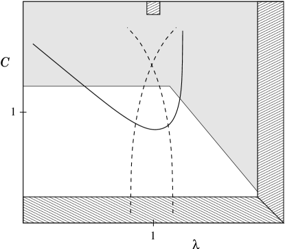
Figure 1: Schematic representation of the limits (hatched) where Eqs.(13), (18) for the viscosity $\eta$ of an emulsion give rigorous results. In the shaded region they predict $\eta$ to be practically independent of capillary number. The frame of the box is meant to comprise the whole $\cal C$-$\lambda$ parameter plane from zero to infinity (small Reynolds number understood). The curved solid line is a sketch of the break–up curve for steadily sheared isolated Newtonian drops according to Grace (1982). Dashed lines indicate schematically our viscosity measurements (see Section 3).

Can we extrapolate the exact second order result Eq.(9) for the stress tensor to arbitrary ${\cal C}$ and $\lambda$ by using the constraints provided by general invariance arguments? For example, since the shear stress has to change sign if the direction of the shear strain is inverted whereas the normal stresses do not, the shear stress and the normal stresses have to be odd/even functions of $\dot{\gamma}$, respectively. From this observation we could have foreseen that Eq.(2) cannot be improved by calculating the next order in $\dot{\gamma}$, i.e., by considering droplet deformation to lowest order. More important are Galilean invariance and invariance under transformations to rotating coordinate frames, which give rise to the material derivative introduced above. Applying the operator $(1+\tau_{1}{\cal D})$ to Eq.(9) adds to the right hand side of the equation a term $2\eta_{T}\tau_{1}{\cal D}e_{ij}$ plus a term of order $O(\dot{\gamma}{\cal C}^{2})$, so that one obtains (in the shear plane)

$$p_{ij}+\tau_{1}{\cal D}\,p_{ij}=2\eta_{T}(e_{ij}+\tau_{2}{\cal D}e_{ij})+\eta_{c}\phi\tau_{1}\dot{\gamma}^{2}\!\frac{25\lambda^{2}+41\lambda+4}{14(2\lambda+3)(\lambda+1)^{2}}\delta_{ij}+O(\dot{\gamma}{\cal C}^{2})\;.$$ (11)

As another short–hand notation we have introduced a second characteristic time $\tau_{2}$, which to the present level of accuracy in $\phi$ is given by

$$\tau_{2}/\tau_{1}=1-\phi\frac{19\lambda+16}{(2\lambda+3)(2\lambda+2)}+O(\phi^{2})\;.$$ (12)

It sets the time scale for strain relaxation in an unstressed region and was named retardation time by Oldroyd (1953). Frankel & Acrivos (1970) realized that up to the partly unknown terms of order $O(\dot{\gamma}{\cal C}^{2})$ on the right–hand side, Eq.(11) belongs to a class of possible viscoelastic equations of state already discussed by Oldroyd (1958). Hence, setting $O(\dot{\gamma}{\cal C}^{2})\equiv 0$ on the right–hand side of Eq.(11), we can define a (minimal) model viscoelastic fluid that behaves identical to the emulsion described by Eq.(9) for small shear rates. In contrast to Eq.(11), the truncated formula for the viscosity

$$\eta=\eta_{T}\frac{1+\tau_{1}\tau_{2}\dot{\gamma}^{2}}{1+(\tau_{1}\dot{\gamma})^{2}}=\frac{\eta_{c}}{1+(\tau_{1}\dot{\gamma})^{2}}\left[1+\phi\frac{5\lambda+2}{2\lambda+2}+\left(1+\phi\frac{5(\lambda-1)}{2\lambda+3}\right)(\tau_{1}\dot{\gamma})^{2}\right]$$ (13)

thus obtained has a manifestly non–perturbative form. However, no phenomenological parameters had to be introduced. Note that Eq.(13) comprises both exactly known limits: ${\cal C}\to 0$ for fixed $\lambda$, and $\lambda\to\infty$ for arbitrary ${\cal C}$. Obviously, Frankel & Acrivos (1970) have forgotten a term $-25\eta_{c}\phi e_{ij}/2$ in their Eq.(3.6) for $p_{ij}$ in the limit $\lambda\to\infty$ for fixed $\cal C$. If the latter is included, Eq.(13) is also in accord with their $O(\lambda^{-1})-$analysis. Moreover, Eq.(13) has the proper limiting behavior for $\lambda=1$, $\sigma\to 0$, i.e. ${\cal C}\to\infty$, which is an extreme case of Eq.(7). Since we assume equal densities for the two phases, the two–phase fluid actually reduces to a one–phase fluid in this degenerate case, and the viscosity is simply $\eta_{c}$, independent of morphology. For illustration, the rigorous limits of Eq.(13) in the ${\cal C}-\lambda$ plane are depicted graphically in Fig. 1. Following Grace (1982), a qualitative break–up curve for single drops under steady shear is also sketched. In summary, Eq.(13) is correct for arbitrary $\lambda$ if ${\cal C}\to 0$, and for arbitrary ${\cal C}$ if $\lambda\to\infty$, and for small and large ${\cal C}$ if $\lambda=1$. Therefore, one can expect that Eq.(13) works reasonably well within a large parameter range (small Reynolds number understood). This is further supported by the observation that the error made in going from Eq.(9) to Eq.(13) rather concerns the shape of the droplet than its extension (it consists in truncating a perturbation series in shape parametrisation). The final result, though sensitive to the latter, is probably less sensitive to the former. Nevertheless, one would not be surprised to see deviations from Eq.(13) when drops become extremely elongated. Finally, due to changes in morphology by break–up and coalescence, the avarage drop size $R$ may change. Observe, however, that for most viscosity ratios ($\lambda$ not close to unity), Eq.(13) is practically independent of capillary number (and thus of $R$) when break–up might be expected according Grace (1982) and others. As an analytic function that is physically known to be bounded from above and from below (the latter at least by the viscosity of a stratified two–phase fluid depicted in Fig. 3), $\eta(\lambda,{\cal C})$ has to have vanishing slope in the ${\cal C}-$direction for large ${\cal C}$. According to Eq.(13), $\eta(\lambda,{\cal C})$ is almost independent of ${\cal C}$ for

$${\cal C}\gg{\cal C}^{*}\approx\frac{40(\lambda+1)}{\sqrt{3}(2\lambda+3)(19\lambda+16)}\;,$$ (14)

where ${\cal C}^{*}$ is the turning point in the dilute limit, determined by $\tau_{1}\dot{\gamma}=1/\sqrt{3}$. For finite volume fractions $\tilde{\tau}_{1}$ from Eq.(16) replaces $\tau_{1}$. Hence, for ${\cal C}\gg{\cal C}^{*}$, Eq.(13) and its extension to higher volume fractions derived below in Eq.(18) are practically independent of drop deformation and morphology. For finite volume fractions a rough interpolation for ${\cal C}^{*}$ derived from Eq.(18) is given by $2.4/(5(1+\phi)+4\lambda)$. In a large part of parameter space we thus expect Eqs.(13), (18) to be applicable to monotonic shear histories with $R$ given by the average initial radius of the droplets. For non–monotonic shear histories, there can of course be hysteresis effects in $\eta(\dot{\gamma})$ that result from morphological changes for ${\cal C}\gg{\cal C}^{*}$. These can only be avoided by substituting for $R$ the radius corresponding to the actual average drop size at the applied shear rate $\dot{\gamma}$.

Figure 2: Self–consistent mean–field description of volume–fraction effects in disordered emulsions and suspensions. The fluid surrounding a test droplet is assumed to have the viscosity $\eta_{c}$ of the continuous phase/the viscosity $\eta$ of the whole emulsion, within/outside the “free–volume–sphere” of radius $R/\phi^{1/3}$.

2.3 Finite volume fractions

A general limitation of the equations discussed so far, is the restriction to small volume fractions. Above, we have implicitly assumed that second order effects from drop interactions are small compared to second order effects from drop deformation. Any direct (coalescence) and indirect (hydrodynamic) interactions of droplets have been neglected in the derivation. Hydrodynamic interactions can approximately be taken into account by various types of cell models. Recently Palierne (1990) proposed a self–consistent method analogous to the Clausius–Mossotti or Lorentz–sphere method of electrostatics. For the case of a disordered spatial distribution of drops his results reduce to those already obtained by Oldroyd (1953). Oldroyd artificially divides the volume around a droplet of viscosity $\eta_{d}\equiv\lambda\eta_{c}$ into an interior “free volume” with a viscosity $\eta_{c}$ of the bare continuous phase and an exterior part with the viscosity $\eta$ of the whole emulsion (see Fig. 2). According to this scheme, an improved version of Eq.(2) should be Oldroyd (1953)

$$\tilde{\eta}_{T}=\eta_{c}\frac{5+3(\eta_{T}/\eta_{c}-1)}{5-2(\eta_{T}/\eta_{c}-1)}\;.$$ (15)

This equation predicts a larger viscosity than its truncation to first order in $\phi$, Eq.(2). Both are shown as dot–dashed lines in Fig. 3. Eq.(15) is qualitatively superior to Eq.(2). We note, however, that the limit $\lambda\to\infty$ deviates in second order in $\phi$ from the result obtained for suspensions by Batchelor & Green (1972). Eq.(15) and likewise all of the following equations containing quantities $\tilde{\eta}_{T}$, $\tilde{\tau}_{1}$, $\tilde{\tau}_{2}$ are only rigorous to first order in $\phi$.

The same reasoning as to the viscosity applies to the characteristic times $\tau_{1}$ and $\tau_{2}$ which now read Oldroyd (1953)

$$\tilde{\tau}_{1}=\frac{\eta_{c}R}{\sigma}\frac{[19\lambda+16][2\lambda+3-2\phi(\lambda-1)]}{40(\lambda+1)-8\phi(5\lambda+2)}\;,$$ (16)

$$\tilde{\tau}_{2}=\frac{\eta_{c}R}{\sigma}\frac{[19\lambda+16][2\lambda+3+3\phi(\lambda-1)]}{40(\lambda+1)+12\phi(5\lambda+2)}\;.$$ (17)

Their ratio $\tilde{\tau}_{2}/\tilde{\tau}_{1}$ is still given by Eq.(12). Finally, Eq.(13) becomes

$$\begin{split}\eta&=\tilde{\eta}_{T}\frac{1+\tilde{\tau}_{1}\tilde{\tau}_{2}\dot{\gamma}^{2}}{1+(\tilde{\tau}_{1}\dot{\gamma})^{2}}\\ &=\frac{\eta_{c}}{1+(\tilde{\tau}_{1}\dot{\gamma})^{2}}\left(\frac{2\lambda+2+3\phi(\lambda+2/5)}{2\lambda+2-2\phi(\lambda+2/5)}+\frac{2\lambda+3+3\phi(\lambda-1)}{2\lambda+3-2\phi(\lambda-1)}(\tilde{\tau}_{1}\dot{\gamma})^{2}\right)\;,\end{split}$$ (18)

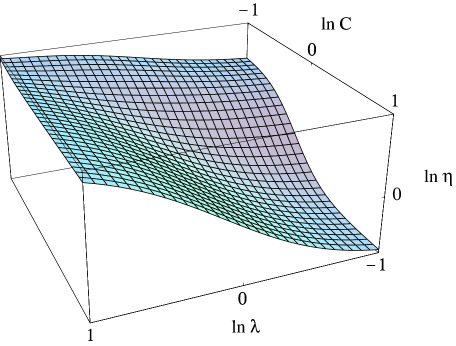
Figure 4: Eq.(18) normalized to $\eta_{c}$ as a function of viscosity ratio $\lambda$ and capillary number ${\cal C}$. The volume fraction of the dispersed phase is chosen to be $\phi=0.3$.

which to our knowledge has not been given before, and is one of our main results. (For a graphical representation see Fig. 4.) In the limit $\tau_{1}\dot{\gamma}\to 0$ it reduces to Eq.(15), whereas for $\tau_{1}\dot{\gamma}\to\infty$ only the second term in parentheses contributes and the curved dashed lines in Fig. 3 are obtained. From the foregoing discussion one should expect Eq.(18) to be applicable within a large range of shear rates, viscosities, and volume fractions.

Finally, we note that more cumbersome expressions for $\tilde{\eta}_{T}$, $\tilde{\tau}_{1}$ and $\tilde{\tau}_{2}$ have been derived within a different cell model by Choi & Schowalter (1975). Here we only quote their expression for $\tilde{\eta}_{T}$,

$$\frac{\tilde{\eta}_{T}}{\eta_{c}}\stackrel{{\scriptstyle C\&S}}{{=}}1+\phi\frac{2[(5\lambda)-5(\lambda-1)\phi^{7/3}]}{4(\lambda+1)-5(5\lambda+2)\phi+42\lambda\phi^{5/3}-5(5\lambda-2)\phi^{7/3}+4(\lambda-1)\phi^{10/3}}$$ (19)

which is also represented graphically by the dotted lines in Fig. 3. Since our data favor Eq.(15) over Eq.(19), and similar observations have been made by others before (see Section 3), we will not pursue this alternative approach further in the present contribution.

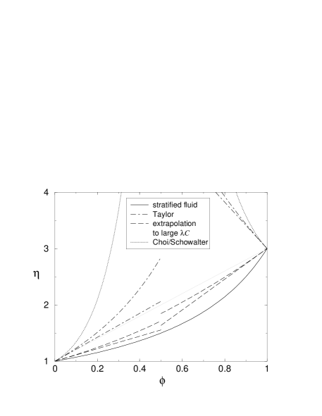
Figure 3: Comparison of different mixing rules for emulsions with viscosity ratio $\lambda=3$ (chosen arbitrarily). The dot–dashed and dashed straight lines pertain to dilute emulsions described by the extrapolation formula Eq.(13), which reduces to Taylor’s formula Eq.(2) for small capillary numbers. The corresponding curved lines are obtained from Eq.(18) where interactions of the droplets are taken into account in a mean–field approximation. The curved dotted lines are the predictions of the cell model by Choi & Schowalter (1975) for small shear rates, Eq.(19). The curved solid line represents the viscosity $\eta=\eta_{c}/[\phi+(1-\phi)\lambda^{-1}]$ of a two–phase stratified fluid and is a lower bound for any viscosity mixing rule.

2.4 A similarity rule

It is interesting to observe that if morphology is conserved (drop size $R$ independent of shear rate) for ${\cal C}\stackrel{{\scriptstyle<}}{{{}_{\sim}}}{\cal C}^{*}$, our Eq.(18) for the nonlinear shear viscosity is closely related to the expressions for the frequency dependent complex viscosity $\eta^{*}(\omega)\equiv\eta^{\prime}(\omega)+\text{i}\eta^{\prime\prime}(\omega)$ of an emulsion of two incompressible Newtonian liquids as derived by Oldroyd (1953),

$$\eta^{*}(\omega)=\tilde{\eta}_{T}\frac{1+\tilde{\tau}_{2}\text{i}\omega}{1+\tilde{\tau}_{1}\text{i}\omega}\;,\qquad\eta^{\prime}(\omega)=\tilde{\eta}_{T}\frac{1+\tilde{\tau}_{1}\tilde{\tau}_{2}\omega^{2}}{1+(\tilde{\tau}_{1}\omega)^{2}}\;,\qquad\eta^{\prime\prime}(\omega)=\tilde{\eta}_{T}\frac{(\tilde{\tau}_{2}-\tilde{\tau}_{1})\omega}{1+(\tilde{\tau}_{1}\omega)^{2}}\;.$$ (20)

For convenience, we also give the corresponding viscoelastic shear modulus $G^{*}(\omega)\equiv\text{i}\omega\,\eta^{*}(\omega)\equiv G^{\prime}(\omega)+\text{i}G^{\prime\prime}(\omega)$,

$$G^{\prime}(\omega)=\omega\tilde{\eta}_{T}\frac{(\tilde{\tau}_{1}-\tilde{\tau}_{2})\omega}{1+(\tilde{\tau}_{1}\omega)^{2}}\;,\qquad G^{\prime\prime}(\omega)=\omega\tilde{\eta}_{T}\frac{1+\tilde{\tau}_{1}\tilde{\tau}_{2}\omega^{2}}{1+(\tilde{\tau}_{1}\omega)^{2}}\;.$$ (21)

Obviously, the shear–rate dependent viscosity of Eq.(18) is obtained from the real part of the complex frequency dependent viscosity $\eta^{*}(\omega)$ by substituting $\dot{\gamma}$ for $\omega$,

$$\eta(\dot{\gamma})\simeq\eta^{\prime}(\omega)\;.$$ (22)

In the same way, the first normal stress difference

$$p_{11}-p_{22}=-2\dot{\gamma}\cdot\phi\,\eta_{c}\,\tau_{1}\,\dot{\gamma}\,\frac{19\lambda+16}{(2\lambda+3)(2\lambda+2)}$$ (23)

from Eq.(9) is obtained to leading order in $\phi$ and $\dot{\gamma}$ from $2\omega\eta^{\prime\prime}(\omega)$, i.e.,

$$p_{11}-p_{22}\simeq 2\omega\eta^{\prime\prime}(\omega)\;.$$ (24)

Reverting the line of reasoning pursued so far, we can conclude that to leading order in ${\cal C}$ and/or $\lambda^{-1}$ the weak deformation limit of the constitutive equation of emulsions is obtained from the linear viscoelastic spectra $G^{\prime}(\omega)$, $G^{\prime\prime}(\omega)$. Further, this identification can possibly be extended (at least approximately) into regions of the ${\cal C}-\lambda$ plane where the critical capillary number for drop breakup is somewhat larger than ${\cal C}^{*}$ of Eq.(14). In hindsight, it is not surprising that in the case of weakly deformed drops the frequency dependent viscosity and the steady shear viscosity are related. Note that under steady shear, drops undergo oscillatory deformations at a frequencey $2\omega=\dot{\gamma}$ if observed from a co–rotating frame turning with vorticity at a frequency $\omega=\dot{\gamma}/2$. If we take Eq.(24) seriously beyond the rigorously known limit, we obtain an interesting prediction for the first normal stress difference. In contrast to Eq.(23), Eq.(24) implies that the first normal stress difference saturates at a finite value $40\,\phi\,\sigma/\!R[2\lambda+3+2\phi(1-\lambda)]^{2}$ for high shear rates. Thus, although the initial slope of the first normal stress difference with $\dot{\gamma}$ increases with $\lambda$, its limit for large $\dot{\gamma}$ decreases with $\lambda$.

Finally, we remark that based on qualitative theoretical arguments, the similarity relation contained in Eq.(22) and Eq.(24) has recently been proposed also for polymer melts Renardy (1997). Usually, in polymer physics a slightly different relation is considered; namely a similarity between $\eta(\dot{\gamma})$ and $|\eta^{*}(\omega)|$, also known as Cox–Merz rule Cox & Merz (1958). In our case, since $\eta^{\prime\prime}\!/\eta^{\prime}=G^{\prime}\!/G^{\prime\prime}=O(\phi)$, we can write

$$\eta(\dot{\gamma})\simeq|\eta^{*}(\omega)|+O(\phi^{2})\;.$$ (25)

Under the conditions mentioned at the beginning of this section, the usual Cox–Merz rule is fulfilled to first order in $\phi$ for an emulsion. Eqs.(22), (24) are interesting from the theoretical point of view, because they suggest a similarity of two a priory rather different quantities. The results of this section also can be of practical use, since they suggest that two different methods may be applied to measure a quantity of interest.

2.5 Non–Newtonian constituents

Generalization of the above theoretical discussion to the case of non–Newtonian constituents is not straightforward. Indeed, as Oldroyd (1953) already knew, his linear–response results quoted in Eq.(20) and Eq.(21) are readily generalized to viscoelastic constituents by replacing the viscosities $\eta_{d,c}$ in the expression for $\eta^{*}$ (or $G^{*}$) by complex viscosities $\eta_{d,c}^{*}(\omega)$ Palierne (1990). As a consequence, the decompositions of $\eta^{*}$ and $G^{*}$ in real and imaginary parts are no longer those of Eqs.(20) and (21), and $\eta^{\prime}$, $\eta^{\prime\prime}$, $G^{\prime}$, $G^{\prime\prime}$ are given by more cumbersome expressions. For the steady–state viscosity, on the other hand, one has to deal with a non–homogeneous viscosity even within homogeneous regions of the emulsion, since the strain rate itself is non–homogeneous and the viscosities are strain rate dependent. We do not attempt to solve this problem here, nor do we try to account for elasticity in the nonlinear case. Yet, it is an intriguing question, whether the similarity rule Eq.(22) can be generalized to the case of non-Newtonian constituents if the constituents themselves obey the Cox–Merz rule (what many polymer melts and solutions do). If both constituents have similar phase angles $\theta\equiv\arctan G^{\prime\prime}\!/G^{\prime}$ the generalized viscosity ratio

$$\lambda^{*}\equiv\frac{\eta_{d}^{*}}{\eta_{c}^{*}}=\frac{|\eta_{d}^{*}|}{|\eta_{c}^{*}|}\text{e}^{\text{i}(\theta_{d}-\theta_{c})}$$ (26)

that enters the expressions for $\eta^{*}$ and $G^{*}$, transforms approximately to $\eta_{d}(\dot{\gamma})/\eta_{c}(\dot{\gamma})$ by applying the Cox–Merz rule. Therefore, in this particular example, Eq.(18) supports the expectation that the generalization may work at least approximately. If, on the other hand, the phase angles of the constituents behave very differently, the answer is less obvious. This problem has been investigated experimentally and is further discussed in Section 3.

In any case, the generalization can only work if the representation of the emulsion by a simple shear–rate dependent viscosity ratio $\eta_{d}(\dot{\gamma})/\eta_{c}(\dot{\gamma})$, with $\dot{\gamma}$ the external shear rate, is justified. In the remainder of this section we construct an argument that allows us to estimate the effective shear–rate dependent viscosity ratio that should replace $\lambda$ in Eq.(18). We take into account the deviation of the strain rate from the externally imposed flow only within the drops, because outside the drops the discrepancy is always small. Inside a drop, the strain rate can be small even for high external shear rates if the viscosity ratio $\lambda=\eta_{d}/\eta_{c}$ is large. Since we are looking for an effective viscosity $\bar{\eta}_{d}(\dot{\gamma})$ for the whole drop to replace the viscosity $\eta_{d}$ at small shear rate, we replace the non–Newtonian drop of non–homogeneous viscosity by an effective pseudo–Newtonian drop of homogeneous but shear–rate dependent viscosity. A possible ansatz for $\bar{\eta}_{d}$ is obtained by requiring that the total energy dissipated within the drop remains constant upon this substitution. Hence, we have

$$\int\!\!dV\;p_{ij}g_{ij}=2\bar{\eta}_{d}\int\!\!dV\;\bar{g}_{ij}\bar{g}_{ij}\;,$$ (27)

where $g_{ij}$ and $\bar{g}_{ij}$ denote the rate–of–strain fields in the real drop and in the corresponding model drop of effective viscosity $\bar{\eta}_{d}$, respectively. They both depend on the position within the drop, whereas the average strain rate

$$\dot{\gamma}^{2}_{\rm eff}\equiv\frac{2}{V}\int\!\!dV\;\bar{g}_{ij}\bar{g}_{ij}$$ (28)

that enters the right–hand side of Eq.(27) does not. Since the strain field $\bar{g}_{ij}$ within a drop of homogeneous viscosity is unique for a given system in a given flow field, $\bar{\eta}_{d}$ itself can be expressed as a function $\bar{\eta}_{d}(\dot{\gamma}_{\rm eff})$ of the average strain rate. Here, we approximate this functional dependence by the strain rate dependence $\eta_{d}(\dot{\gamma})$ of the viscosity of the dispersed fluid. Further, neglecting drop deformation we calculate $\dot{\gamma}_{\rm eff}$ from the velocity field within a spherical drop Bartok & Mason (1958) and obtain

$$\bar{\lambda}\equiv\frac{\bar{\eta}_{d}(\dot{\gamma}_{\rm eff})}{\eta_{c}(\dot{\gamma})}\approx\frac{\eta_{d}\left(\sqrt{2}\dot{\gamma}/(\bar{\lambda}+1)\right)}{\eta_{c}(\dot{\gamma})}\;.$$ (29)

A different prefactor ($\sqrt{7}$ in place of $\sqrt{2}$) in the expression for the effective strain rate $\dot{\gamma}_{\rm eff}$ was obtained by de Bruijn (1989) using instead of the average in Eq.(28) the maximum norm of $\bar{g}_{ij}$. To obtain the correction to Eq.(18) due to Eq.(29) in the case of non–Newtonian constituents, the implicit equation for $\bar{\lambda}$ has to be solved for given functions $\eta_{c}(\dot{\gamma})$ and $\eta_{d}(\dot{\gamma})$. For shear thinning constituents, Eq.(29) implies a tendency of Eq.(18) to overestimate $\eta(\dot{\gamma})$ if $\dot{\gamma}$ and $\lambda$ are large. In the actual case of interest, for the constituents that were used in the experiments discussed in Section 3, the viscosity ratio $\lambda$ ($\eta_{d}$ and $\eta_{c}$ taken at the external shear rate $\dot{\gamma}$) varies almost by a factor of 10. However, the corrections discussed in this Section only become important for high shear rates, where the constituents are shear thinning. In this regime, the viscosity ratio (viscosities taken at the external shear rate) only varies between $1/2$ and $2$, and hence the corrections expected from Eq.(29) are at best marginally significant at the level of accuracy of both Eq.(29) and the present measurements. Therefore, a representation of the drops by pseudo–Newtonian drops of homogeneous but shear–rate dependent viscosity is most probably not a problem for the measurements presented in the following section. The question as to a generalization of the similarity rule Eq.(22) to non–Newtonian constituents seems well defined.

3 Experiment

3.1 Materials and methods

The experimental investigation deals with a phase separated aqueous solution containing a polysaccharide (alginate) and a protein (caseinate). This type of solutions are currently used in the food industry. The methods for characterizing the individual polymers in solution are in general known, especially when dealing with non–gelling solutions where composition and temperature are the only relevant parameters. The polymers are water soluble. When the two biopolymers in solution are mixed, a miscibility region appears in the low concentrations range and phase separation at higher concentrations. The binodal and the tie lines of the phase diagram can then be established by measuring the composition of each phase at a fixed temperature. In general, the rheological behavior of phase separated systems is difficult to investigate, and a suitable procedure is not fully established. In some cases, two–phase solutions macroscopically separate by gravity within a short period of time, but in some other cases (such as ours) they remain stable for hours or days without appearance of any visible interface. These “emulsion type” solutions have no added surfactant. Following approaches developed for immiscible blends, one may try to characterize the partially separated solution as an effective emulsion if the coarsening is slow enough. In order to establish a comparison between phase separated solutions and emulsions, it is necessary to know

• the volume fraction of the phases,

• their shear–rate dependent viscosities (flow curves),

• their viscoelastic spectra,

• the interfacial tension $\sigma$ between the phases,

• the average radius of $R$ the drops

Only the ratio $R/\sigma$ enters rheological equations. Knowledge of either $R$ or $\sigma$ allows the other quantity to be inferred from rheological measurements.

A difficulty when working with phase separated solutions, as opposed to immiscible polymer melts, arises from the fact that each phase is itself a mixture (and not a pure liquid) and therefore the rheology of the phase depends on its particular composition. If one wishes to minimize the number of parameters, it is important to keep the composition of the phases constant upon changing the volume fractions. This can be achieved by working along a tie line of the phase diagram. And this is precisely the procedure that we followed. The polymers were first dissolved, then a large quantity of the ternary mixture was prepared (350 ml) and was centrifuged. The two phases were then collected separately. Both pure phases were found to be viscoelastic and to exhibit shear thinning behavior, which is especially pronounced for the alginate rich phase with $\eta(10^{-1}\;\text{s}^{-1})/\eta(10^{3}\;\text{s}^{-1})\approx 20$, while the caseinate rich phase is almost Newtonian below $10^{2}$ s^-1. The viscosity of the alginate rich phase is higher than that of the caseinate rich phase for shear rates below $2\cdot 10^{2}$ s^-1 and lower for higher shear rates. We checked that both phases obey the usual Cox–Merz rule in the whole range of applied shear rates.

By mixing various amounts of each phase, the volume fraction of the dispersed phase was varied between $10\,\%$ and $30\,\%$ while the composition of each phase was kept constant. In particular, the temperature was kept constant and equal to the centrifugation temperature in order to avoid redissolution of the constituents. To prepare the emulsion, the required quantities of each phase were mixed in a vial and gently shaken. Then the mixture was poured on the plate of the rheometer (AR 1000 from TA Instruments fitted with a cone and plate geometry 6 cm/$2^{\circ}$) and a constant shear rate was applied. The apparent viscosity for a particular shear rate was then recorded versus time until it reached a stable value. By shearing at a fixed shear rate, one may expect to create a steady size distribution of droplets, with a shear rate dependent average size. After each shear experiment a complete dynamic spectrum was performed. In this way, shear rates ranging between $3\cdot 10^{-2}$ s^-1 and $10^{3}$ s^-1 were applied. The analysis of each spectrum according to Palierne (1990) allowed us to derive by curve fitting the average drop radius $R$ at the corresponding shear rate.

More technical details about the experimental investigation along with more experimental results will be presented elsewhere. Here, we concentrate on the analysis of those aspects of the rheological measurements pertinent to the theoretical discussion in Section 2.

3.2 Results and discussion

In this section we present our experimental observations and address the questions posed at the end of the introduction. Before we present our own data we want to comment briefly on related data recently obtained for polymer melts by Grizzuti & Buonocore (1998). These authors measured the shear–rate dependent viscosity of binary polymer melts and compared them to the low volume fraction limit of Eq.(18), i.e. Eq.(13), and to (a truncated form of) results of Choi & Schowalter (1975). They reported much better agreement with Eq.(13) than with the truncated series from Choi & Schowalter (1975). Comparison with the full expressions of Choi & Schowalter (1975) would have made the disagreement even worse (cf. Fig 3). The average radius $R$ that enters the equation, was determined independently for each shear rate applied. The constituents where moderately non–Newtonian polymer melts, the viscosity ratio varying between $\lambda\approx 0.3\dots 3$ over the range of shear rates applied. Hence, these experiments, are located in the interesting parameter range, where Eqs.(18) and Eq.(13) for $\eta(\dot{\gamma})$ are expected to be sensitive to drop deformation and break–up. Surprisingly, the results show that they describe the data very well over the whole range of shear rates although one would not necessarily expect average drop deformation to be very small. Unfortunately, drop sizes have not been reported by the authors, so conclusions concerning the location in the ${\cal C}-\lambda$ parameter plane and the validity of the similarity rule Eq.(22) cannot be drawn. Also the question, whether Eq.(18) holds for small viscosity ratios $\lambda\ll 0.3$, cannot be answered.

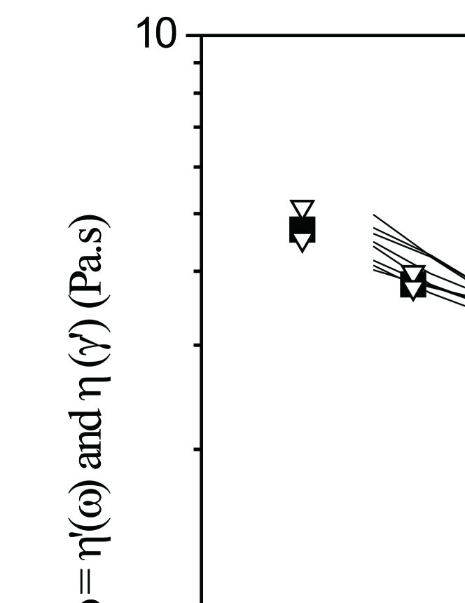
Figure 5: The nonlinear shear viscosity $\eta(\dot{\gamma})$ (opaque squares) and the real part $\eta^{\prime}(\omega)$ of the dynamic viscosity $\eta^{*}(\omega)$ (lines) of a droplet phase of a mixture of weakly viscoelastic polymer solutions (alginate/caseinate). Also shown is Eq.(18) for the viscosity of an emulsion of Newtonian constituents evaluated for the actually non–Newtonian viscosities of the constituting phases with the drop size obtained from the spectra (open triangles). Due to the scatter in the dynamic viscosity at low frequencies there is an uncertainty in the average drop size, resulting in corresponding error bars (multiple points) for Eq.(18).

Our own measurements were located in about the same $\lambda-$range. As we noted in the preceding section, only the ratio $R/\sigma$ enters rheological equations and knowledge of either $R$ or $\sigma$ allows the other quantity to be inferred from rheological measurements. Ding & Pacek (1999) determined the interfacial tension of the alginate/caseinate system used in our experiments by observing drop relaxation under a microscope and analyzing the data according to Section 2. They found $\sigma\simeq 10^{-5}$ N/m. Using this, we obtained an average drop size $R\simeq 10^{-5}$ m from the measured spectra $G^{\prime}(\omega)$, $G^{\prime\prime}(\omega)$ according to Palierne (1990) for the experiments reported in Fig. 5. By the method based on Palierne (1990), we could not detect a decrease in drop size with shear rate as expected from the phenomenological phase diagram for single Newtonian drops under shear as established by Grace (1982) and others. Thus, the limit of high capillary numbers and moderate viscosity ratios (the region above the break–up curve) in Fig. 1 has been accessed experimentally. Corresponding locations have been indicated qualitatively in the figure by dashed lines. With the drop size being constant, one can try to test the proposed similarity rule Eq.(22). By identifying the axis for frequency $\omega$ and shear rate $\dot{\gamma}$, data for the real part $\eta^{\prime}(\omega)$ of the frequency dependent dynamic viscosity $\eta^{*}(\omega)$ are compared to data for the shear–rate dependent viscosity $\eta(\dot{\gamma})$ in Fig. 5. The emulsion containing $30\,\%$ of the alginate rich phase and $70\,\%$ of the caseinate rich phase has been prepared at room temperature as described in the preceding section. Steady shear rates ranging between $3\cdot 10^{-2}$ s^-1 and $10^{3}$ s^-1 corresponding to capillary numbers ${\cal C}\approx 6\cdot 10^{-2}\dots 10^{3}$ have been applied. The shear viscosity (opaque squares) is reported in the figure for each of these individual measurements. The multiple data sets for $\eta^{\prime}$ (lines) taken each between two successive steady shear measurements, superimpose fairly well; i.e. the spectra appear to be remarkably independent of the preceding steady shear rate. The good coincidence of $\eta^{\prime}(\omega)$ and $\eta(\dot{\gamma})$ in Fig. 5 show that the data obey the proposed similarity rule Eq.(22) over a large range of shear rates. The agreement near $\dot{\gamma}\approx 2\cdot 10^{2}$ s^-1 is a consequence of the proximity to the trivial limit $\lambda=1$, ${\cal C}=\infty$. Nevertheless, the data provide strong evidence that Eq.(22) is an excellent approximation for a large range of viscosity ratios and capillary numbers. Similar results (not shown) have been obtained for other volume fractions. Comparison with Eq.(18) represented by the open triangles in Fig. 5, on the other hand, is less successful at large shear rates, although it is still not too far off for a theoretical curve without any adjustable parameter. A discrepancy had to be expected as a consequence of the non–Newtonian character of the constituents at large shear rates, which is definitely not taken into account in Eq.(18). For the plot of Eq.(18) in Fig. 5 we merely substituted $\eta_{d}(\dot{\gamma})/\eta_{c}(\dot{\gamma})$ taken at the external shear rate $\dot{\gamma}$ for $\lambda$. The average drop size $R$ was obtained from fitting the viscoelastic moduli. The scatter in the dynamic viscosity data gives rise to an uncertainty in $R$, which is reflected by the multiple open triangles at low shear rates. It seems that the similarity rule Eq.(22) is more general than Eq.(18), i.e., it still holds for rather viscoelastic constituents (that obey the usual Cox–Merz rule), where the latter fails. This relation certainly deserves further investigation with different materials and methods.

In summary, we have succeeded in establishing an analogy first between a partially phase–separated polymer solution and an emulsion, and further between the viscoelastic spectrum of the system and its nonlinear shear viscosity even in the case of (moderately) non–Newtonian constituents.

This work was supported by the European Community under contract no FAIR/CT97-3022. We thank P. Ding and A. W. Pacek (University of Birmingham) for measuring the surface tension and S. Costeux and G. Haagh for helpful discussions and suggestions.

References

- Bartok & Mason (1958) Bartok, W. & Mason, S. G. 1958 Particle motions in sheared suspensions. J. Colloid Sci. 13, 293.
- Batchelor & Green (1972) Batchelor, G. K. & Green, J. T. 1972 The determination of the bulk stress in a suspension of spherical particles to order . J. Fluid Mech. 56, 401.
- de Bruijn (1989) de Bruijn, R. A. 1989 Deformation and breakup of drops in simple shear flows. PhD thesis, TU Eindhoven, The Netherlands.
- Choi & Schowalter (1975) Choi, S. J. & Schowalter, W. R. 1975 Rheological properties of nondilute suspensions of deformable particles. Phys. Fluids 18, 420.
- Cox & Merz (1958) Cox, W. P. & Merz, E. H. 1958 Correlation of dynamic and steady flow viscosities. J. Polym. Sci. 28, 619.
- Ding & Pacek (1999) Ding, P. & Pacek, A. W. 1999 unpublished.
- Frankel & Acrivos (1970) Frankel, N. A. & Acrivos, A. 1970 The constitutive equation for a dilute emulsion. J. Fluid Mech. 44, 65.
- Grace (1982) Grace, H. P. 1982 Dispersion phenomena in high viscosity immiscible fluid systems and application of static mixers as dispersion devices in such systems. Chem. Eng. Commun. 14, 225.
- Grizzuti & Buonocore (1998) Grizzuti, N. & Buonocore, G. 1998 The morphology-dependent rheological behavior of an immiscible model polymer blend. In Proceedings of the European Rheology Conference (ed. I. Emri & R. Cvelbar), Progress and Trends in Rheology, vol. 5, p. 80. Darmstadt: Steinkopff.
- Oldroyd (1950) Oldroyd, J. G. 1950 On the formulation of rheological equations of state. Proc. Roy. Soc. A 200, 523.
- Oldroyd (1953) Oldroyd, J. G. 1953 The elastic and viscous properties of emulsions and suspensions. Proc. Roy. Soc. A 218, 122.
- Oldroyd (1958) Oldroyd, J. G. 1958 Non-newtonian effects in steady motion of some idealized elasto-viscous liquids. Proc. Roy. Soc. A 245, 278.
- Palierne (1990) Palierne, J. F. 1990 Linear rheology of viscoelastic emulsions with interfacial tension. Rheol. Acta 29, 204.
- Rallison (1980) Rallison, J. M. 1980 Note on the time-dependent deformation of a viscous drop which is almost spherical. J. Fluid Mech. 98, 625.
- Renardy (1997) Renardy, M. 1997 Qualitative correlation between viscometric and linear viscoelastic functions. J. Non-Newtonian Fluid Mech. 68, 133.
- Schowalter et al. (1968) Schowalter, W. R., Chaffey, C. E. & Brenner, H. 1968 Rheological behavior of a dilute emulsion. J. Colloid and Interface Sci. 26, 152.
- Taylor (1932) Taylor, G. I. 1932 The viscosity of a fluid containing small drops of another fluid. Proc. Roy. Soc. A 138, 41.
- Taylor (1934) Taylor, G. I. 1934 The formation of emulsions in definable fields of flow. Proc. Roy. Soc. A 146, 501.