When do finite sample effects significantly affect entropy estimates ?

Abstract

An expression is proposed for determining the error made by neglecting finite sample effects in entropy estimates. It is based on the Ansatz that the ranked distribution of probabilities tends to follow a Zipf scaling.

1 Introduction

The growing interest in complexity measures and symbolic dynamics [1, 2] has brought to the forefront various problems related to the estimation of entropic quantities from finite sequences [3]. Such estimates are known to suffer from a bias, which prevents quantities such as the metric entropy from being meaningfully estimated. The purpose of this letter is to provide an analytical expression for this bias,in order in order to test for finite sample effects in entropy estimates.

Consider the general case of a string of $N$ symbols $\{i_{1}i_{2}\cdots i_{N}\}$, each of which belongs to a finite alphabet ${\mathcal{A}}$. The average informational content of substrings of length $d$ taken from this sequence is expressed by the Shannon entropy [4]

$$H_{d}=-\sum_{i_{1},\ldots,i_{d}\in{\mathcal{A}}}\mu\left([i_{1}i_{2}\cdots i_{d}]\right)\log\mu\left([i_{1}i_{2}\cdots i_{d}]\right)\ ,$$ (1)

where $\mu$ is the natural invariant measure with respect to the shift. Of particular interest is the block or dynamical Shannon entropy $h_{d}=H_{d+1}-H_{d}$ from which one gets the measure-theoretic entropy of the system

$$h(\mu)=\lim_{d\rightarrow\infty}h_{d}\ ,$$ (2)

a quantity that is intimately related to the Kolmogorov-Sinaï entropy in case the string represents the output of a shift dynamical system.

The main problem lies in the estimation of the empirical measure $\mu$ from a finite string of symbols. Direct box counting yields

$$\mu\left([i_{1}i_{2}\cdots i_{d}]\right)\approx\frac{\#[i_{1}i_{2}\cdots i_{d}]}{N-d+1}\ ,$$ (3)

where $\#[i_{1}i_{2}\cdots i_{d}]$ is the occurrence frequency of the block $i_{1}i_{2}\cdots i_{d}$ in the string. It is well known that statistical fluctuations in the sample on average lead to a systematic underestimation of the entropy. This problem becomes particularly acute as the word size increases for a given string length $N$. Since this deviation can easily be mistaken for the signature of a finite memory process, it is of prime importance to determine whether its origin is physical or not.

Several authors have already addressed the problem of making corrections to empirical entropy estimates [3, 5, 6, 7]; their expressions are valid as long as the occurrence frequencies of the observed words are large compared to one. While this may hold for relatively short words, it breaks down for long ones, making it difficult for a small correction to be used as a safe indication for a small deviation. Our objective is to derive a more reliable (although less accurate) expression of the deviation, to be used as a warning signal against the onset of finite sample effects.

As a first guess one could require the sample to be long enough for each word to have a chance to appear. This gives $N\gg N_{\textrm{\scriptsize symb}}^{d}$, where $N_{\textrm{\scriptsize symb}}$ is the cardinality of the alphabet. This criterion, however, is generally found to be too conservative because it does not take into account the grammar, i.e. the rules that cause some words to be forbidden or less frequent than others.

2 The Zipf-ordered distribution

To derive our expression, we first rank the words according to their frequency of occurrence: let $n_{k=1}$ denote the frequency of occurrence of the most probable word, $n_{k=2}$ of the next most probable one etc. Multiple instances of the same frequency get consecutive ranks. This monotonically decreasing distribution is called Zipf-ordered.

The Asymptotic Equipartition Property introduced by Shannon [4] states that the ensemble of words of length $d$ can be divided into two subsets. The first one consists of “typical words” that occur frequently and roughly have the same probability of occurrence. The other subset is made of “rare words” that belong to the tail of the distribution. According to the Shannon-Breiman-MacMillan theorem, the entropy is related to the typical words in the limit where $N\rightarrow\infty$; the contribution of rare words progressively disappears as $N$ increases. In some sense this observation justifies the procedure to be described below.

It was noted by Pareto [8], Zipf [9] and others, and later interpreted by Mandelbrot [10] that the tail of the Zipf-ordered distribution $n_{k}$ tends to follow a universal scaling law

$$n_{k}=\alpha k^{-\gamma}\ ,\ \ \gamma>0\ .$$ (4)

which is found with astonishing reproducibility in economics, social sciences, physics etc. [10]. As shown in [11, 12], many different systems give rise to Zipf laws, whose ubiquity is thought to be essentially a consequence of the ranking procedure.

The physical meaning of Zipf’s law is still an unsettled question, although it does not seem to reflect any particular self-organization (see for example [13, 14]). We just mention that a slow decay is an indication for a “rich vocabulary”, in the sense that rare words occur relatively often.

The key point is that the empirical Zipf-ordered distribution has a cutoff at some finite value $k=N_{\textrm{\scriptsize max}}$ because of the finite length of the symbol string. For the same reason, the occurrence frequencies are necessarily quantized. Our main hypothesis is that the true distribution extends beyond $N_{\textrm{\scriptsize max}}$, up to the lexicon size $K\geq N_{\textrm{\scriptsize max}}$, following Zipf’s law with the same exponent $\gamma$. This Ansatz has already been suggested as a way to estimate entropies from long words [15].

3 Estimating the bias

Let $\hat{H}$ be the Shannon entropy computed from the empirical distribution (using eqs. 1 and 3) and $H$ the entropy one would obtain from a non truncated distribution, in which the frequencies are not quantized anymore and extend beyond $N_{\textrm{\scriptsize max}}$ following Zipf’s law.

$$\hat{H} = -\sum_{k=1}^{N_{\textrm{\tiny max}}}\frac{n_{k}}{\sum_{k=1}^{N_{\textrm{\tiny max}}}n_{k}}\log\frac{n_{k}}{\sum_{k=1}^{N_{\textrm{\tiny max}}}n_{k}}\ ,$$ (5)

$$H = -\sum_{k=1}^{K}\frac{n_{k}}{\sum_{k=1}^{K}n_{k}}\log\frac{n_{k}}{\sum_{k=1}^{K}n_{k}}\ .$$

The truncation has two counteracting effects. It changes the renormalization of the occurrence frequencies and causes some of the least frequent words to be omitted.

The difference $\delta$ between the two entropy estimates

$$\delta=H-\hat{H}\ .$$ (6)

is what we call the bias, to be used as a measure of the deviation resulting from finite sample effects. We shall assume that $N_{\textrm{\scriptsize max}}\gg 1$, which is equivalent to saying that the distribution must have a sufficiently long tail for a power law to make sense.

It is natural to define a small parameter $0\leq\varepsilon\ll 1$, which goes to zero for a non truncated distribution

$$\varepsilon=\frac{1}{N}\sum_{k=N_{\textrm{\tiny max}}+1}^{K}n_{k}\ .$$ (7)

Remember that $N=\sum_{k=1}^{K}n_{k}$ [16].

Now, assuming that Zipf’s law persists for $k>N_{\textrm{\scriptsize max}}$, we have

$$\varepsilon=\frac{1}{N}\!\sum_{k=N_{\textrm{\tiny max}}+1}^{K}\alpha k^{-\gamma}=\frac{\alpha}{N}\big{(}\zeta(\gamma,N_{\textrm{\scriptsize max}}+1)-\zeta(\gamma,K+1)\big{)}\ ,$$ (8)

where $\zeta(\gamma,m)$ is the Hurwitz or generalized Riemann zeta function. For $k>\gamma$, the following approximation holds [17]

$$\zeta(\gamma,m)=\frac{m^{1-\gamma}}{\gamma-1}-\frac{m^{-\gamma}}{2}+\frac{m^{-\gamma-1}}{12}\ .$$ (9)

Since $K,N_{\textrm{\scriptsize max}}\gg 1$, we may write

$$\varepsilon=\frac{\alpha}{N(\gamma-1)}\left({N_{\textrm{\scriptsize max}}^{1-\gamma}-K^{1-\gamma}}\right)\ .$$ (10)

The value of $\alpha$ remains to be determined. To do so, we note that the least frequent words in the Zipf-ordered distribution occur once or a few times only. One may therefore reasonably set $n_{k=N_{\textrm{\tiny max}}}\approx 1$, giving $\alpha\approx N_{\textrm{\scriptsize max}}^{\gamma}$.

The bias $\delta$ can now be expanded in powers of $\varepsilon$. Keeping terms of order ${\mathcal{O}}(\varepsilon)$ only, we have

$$\delta=-\varepsilon\hat{H}+(1+\varepsilon)\left(\varepsilon-\sum_{k=N_{\textrm{\tiny max}}+1}^{K}\frac{n_{k}}{N}\log\frac{n_{k}}{N}\right)\ .$$ (11)

For the conditions stated before, the sum can be approximated by

$$\sum_{k=N_{\textrm{\tiny max}}+1}^{K}\frac{n_{k}}{N}\log\frac{n_{k}}{N}=-\varepsilon\left(\log N-\gamma\log\frac{N_{\textrm{\scriptsize max}}}{K}\right)\ ,$$ (12)

finally giving the result of interest

$$\delta = \varepsilon\left(1+\log N-\hat{H}-\gamma\log\frac{N_{\textrm{\scriptsize max}}}{K}\right)$$ (13)

$$\varepsilon \approx \frac{N_{\textrm{\scriptsize max}}}{N(\gamma-1)}\left(1-\left(\frac{N_{\textrm{\scriptsize max}}}{K}\right)^{\gamma-1}\right)\ .$$

Notice that the true entropy is always underestimated; furthermore $\varepsilon$ is continuous at $\gamma=1$ [18]. Most of the variation comes from the small parameter $\varepsilon$, whose expression reveals two different effects :

1. the ratio $N_{\textrm{\scriptsize max}}/N$ reflects the uncertainty of the frequency estimates.

2. the scaling index $\gamma$, whose value is usually between 0.5 to 1.5, is indicative of the lacunarity of the word distribution. In the case of a shift dynamical system, $\gamma$ reveals how unevenly the rare orbits fill the phase space.

For the sake of comparison, the first order approximation for finite sample effects derived in [5, 6] is

$$\delta=\frac{N_{\textrm{\scriptsize max}}}{2N}\ .$$ (14)

We conclude from eq. 13 that the bias is not just related to statistical fluctuations in the empirical occurrence frequency, but is also caused by the omission of words that are asymptotically rare. If the true distribution of the ranked words were exponential or ultimately ended with an exponential tail, then our criterion would be too conservative but still reliable as such.

The following procedure is proposed for detecting the maximum word length for which entropies can be meaningfully estimated : compute Zipf-ordered distributions for increasing word-lengths $d$. For each length, estimate the bias $\delta$ by least-squares fitting a power law to the tail of the observed distribution. As soon as this bias exceeds a given threshold (say 10% of $\hat{H}$), then entropies computed from longer words are likely to be significantly corrupted by finite sample effects.

Equation 13 supposes that the maximum lexicon size $K$ is known a priori, which is seldom the case. This is not a serious handicap, however, since the value of $K$ has relatively little impact on the bias; a rough approximation such as $K=N_{\textrm{\scriptsize symb}}^{d}$ may do well.

4 Two examples

To briefly illustrate the results, we now consider two examples. The first one is based on a Bernouilli process, whose entropy and Zipf-ordered distribution can be calculated analytically. The string of symbols is drawn from a two letter alphabet, one with probability $\lambda$ and the other with probability $1-\lambda$. The block entropy of this process is independent of the word length and equals

$$h=-\lambda\log\lambda-(1-\lambda)\log(1-\lambda)\ .$$ (15)

Figure 1 compares the true block entropy with estimates drawn from a sample of length $N=2000$ with $\lambda=0.15$. The departure of the empirical estimate from the true one is evident. Without knowledge of the true entropy, however, it is very difficult to tell whether the decrease of the entropy is an artifact or just the signature of a short-time memory.

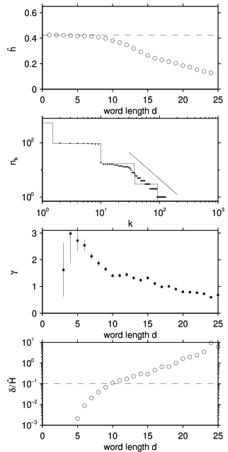
Figure 1: Analysis of a Bernouilli sequence, with $N=2000$ and $\lambda=0.15$. From top to bottom: (1) the empirical block entropy and the true one (dashed), (2) the true (line) and observed (dots) Zipf-ordered distributions for words of length $d=8$; (3) the scaling exponent $\gamma$ obtained by fitting the tail of the Zipf-ordered distribution (error bars represent $\pm 1$ standard deviation resulting from the least-squares fit), (4) the bias $\delta$. In this case, entropies cannot be reliably estimated for word lengths beyond $d=9$. Block entropies are normalized to $\log N_{\textrm{\scriptsize symb}}$, so that the maximum possible value is 1.

The second panel displays the true and the empirical Zipf-ordered distributions as obtained for words of length $d=9$. Zipf’s law clearly holds for words whose rank exceeds about 30. After this, the scaling exponent $\gamma$ is estimated, see the third panel. The decrease of this exponent with the word length $d$ suggests that the contribution of the rare words becomes increasingly important. Finally, the bias $\delta$, which is shown in the fourth panel, suggests that the onset of a significant bias occurs around $d=8$; this value is indeed in agreement with the results of the first panel.

The validity of the bias estimate was tested on various examples and was found to be reliable, provided that $N_{\textrm{\scriptsize max}}\gg 1$.

In the second example, we consider a sequence of $N=10^{4}$ symbols generated by the logistic map $x_{i+1}=\lambda x_{i}(1-x_{i})$ in a chaotic regime with $\lambda=3.8$. The (generating) partition ${\mathcal{P}}=\{[0,0.5[,[0.5,1]\}$ gives us a two-letter alphabet.

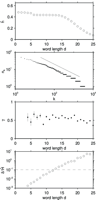
Figure 2: Analysis of a logistic map sequence, with the same legend as the previous figure; the string length is $N=10^{4}$. The second panel shows a Zipf-ordered distribution for $d=18$. The largest word size for which the relative bias is smaller than 10$\%$, is $d=12$.

Figure 2 again shows that the block entropy decreases above a certain word length. In contrast to the previous example, the measured scaling exponent $\gamma$ is small and almost constant, regardless of the word length. We believe this to be a consequence of the intricate structure of the self-similar attractor. This low value of $\gamma$ already suggests that rare words should bring a significant contribution to the entropy. The bias $\delta$ finally suggests stopping at $d=12$.

5 Conclusion

Summarizing, we have derived a simple expression (eq. 13) for detecting the onset of finite sample size effects in entropy estimates. It is based on the empirical evidence that rank-ordered distribution of words tend to follow Zipf’s law. The criterion reveals that rare events can significantly bias the empirical entropy estimate.

References

- [1] C. Beck and F. Schlögl, Thermodynamics of chaotic systems (Cambridge University Press, Cambridge, 1993).
- [2] R. Badii and A. Politi, Complexity: hierarchical structures and scaling in physics (Cambridge University Press, Cambridge, 1997).
- [3] T. Schürmann and P. Grassberger, Chaos 6, 414 (1996).
- [4] R. E. Blahut, Principles and practice of information theory (Addison Wesley, Reading, MS, 1987).
- [5] H. Herzel, Sys. Anal. Mod. Sim. 5, 435 (1988).
- [6] P. Grassberger, Phys. Lett. A 128, 369 (1988).
- [7] A. O. Schmitt, H. Herzel, and W. Ebeling, Europhys. Lett. 23, 303 (1993).
- [8] V. Pareto, Cours d’économie politique (Rouge, Lausanne, 1897).
- [9] G. Zipf, Human behavior and the principle of least effort (Addison-Wesley, Cambridge MA, 1949).
- [10] B. Mandelbrot, Fractals and scaling in finance: discontinuity, concentration, risk (Springer, New York, 1997); B. Mandelbrot, Fractales, hasard et finance (Flammarion, Paris, 1997).
- [11] R. Günther, L. Levitin, B. Schapiro, and P. Wagner, Int. J. Theor. Physics 35, 395 (1996).
- [12] G. Troll and P. beim Graben, Phys. Rev. E 57, 1347 (1998).
- [13] G. A. Miller and E. B. Newman, Am. J. Psychology 71, 209 (1958).
- [14] W. Li, Complexity 3, 10 (1998).
- [15] T. Pöschel, W. Ebeling and H. Rosé, J. Stat. Phys. 80, 1443 (1995).
- [16] To be exact , but we use the fact that .
- [17] J. Spanier and K. B. Oldham, An atlas of functions (Springer, Berlin, 1987), formula 64:9:1.
- [18] The term can be large when and but this divergence becomes effective long after the maximum word size has been exceeded; it is therefore not a matter of concern here.