Physics of Particle Detection

Abstract

In this review the basic interaction mechanisms of charged and neutral particles are presented. The ionization energy loss of charged particles is fundamental to most particle detectors and is therefore described in more detail. The production of electromagnetic radiation in various spectral ranges leads to the detection of charged particles in scintillation, Cherenkov and transition radiation counters. Photons are measured via the photoelectric effect, Compton scattering or pair production, and neutrons through their nuclear interactions.

A combination of the various detector methods helps to identify elementary particles and nuclei. At high energies absorption techniques in calorimeters provide additional particle identification and an accurate energy measurement.

Introduction

The detection and identification of elementary particles and nuclei is of particular importance in high energy, cosmic ray and nuclear physics r:cgru:[1] ; r:cgru:[2] ; r:cgru:[3] ; r:cgru:[4] ; r:cgru:[5] ; r:cgru:[6] . Identification means that the mass of the particle and its charge is determined. In elementary particle physics most particles have unit charge. But in the study e.g. of the chemical composition of primary cosmic rays different charges must be distinguished.

Every effect of particles or radiation can be used as a working principle for a particle detector.

The deflection of a charged particle in a magnetic field determines its momentum $p$; the radius of curvature $\rho$ is given by

$$\rho\propto\frac{p}{z}=\frac{\gamma m_{0}\beta c}{z}$$ (1)

where $z$ is the particle’s charge, $m_{0}$ its rest mass and $\beta=\frac{v}{c}$ its velocity. The particle velocity can be determined e.g. by a time-of-flight method yielding

$$\beta\propto\frac{1}{\tau}\quad,$$ (2)

where $\tau$ is the flight time. A calorimetric measurement provides a determination of the kinetic energy

$$E^{\rm kin}=(\gamma-1)m_{0}c^{2}$$ (3)

where $\gamma=\frac{1}{\sqrt{1-\beta^{2}}}$ is the Lorentz factor.

From these measurements the ratio of $m_{0}/z$ can be inferred, i.e. for singly charged particles we have already identified the particle. To determine the charge one needs another $z$-sensitive effect, e.g. the ionization energy loss

$$\frac{{\rm d}E}{{\rm d}x}\propto\frac{z^{2}}{\beta^{2}}\ln(a\beta\gamma)$$ (4)

($a$ is a material dependent constant.)

Now we know $m_{0}$ and $z$ separately. In this way even different isotopes of elements can be distinguished.

The basic principle of particle detection is that every physics effect can be used as an idea to build a detector. In the following we distinguish between the interaction of charged and neutral particles. In most cases the observed signature of a particle is its ionization, where the liberated charge can be collected and amplified, or its production of electromagnetic radiation which can be converted into a detectable signal. In this sense neutral particles are only detected indirectly, because they must first produce in some kind of interaction a charged particle which is then measured in the usual way.

Interaction of Charged Particles

Kinematics

Four-momentum conservation allows to calculate the maximum energy transfer of a particle of mass $m_{0}$ and velocity $v=\beta c$ to an electron initially at rest to be r:cgru:[2]

$$E^{\rm max}_{\rm kin}=\frac{2m_{e}c^{2}\beta^{2}\gamma^{2}}{1+2\gamma\frac{m_{e}}{m_{0}}+\left(\frac{m_{e}}{m_{0}}\right)^{2}}=\frac{2m_{e}p^{2}}{m_{0}^{2}+m_{e}^{2}+2m_{e}E/c^{2}}\quad,$$ (5)

here $\gamma=\frac{E}{m_{0}c^{2}}$ is the Lorentz factor, $E$ the total energy and $p$ the momentum of the particle.
For low energy particles heavier than the electron ($2\gamma\frac{m_{e}}{m_{0}}\ll 1$; $\frac{m_{e}}{m_{0}}\ll 1$) eq. 5 reduces to

$$E^{\rm max}_{\rm kin}=2m_{e}c^{2}\beta^{2}\gamma^{2}\quad.$$ (6)

For relativistic particles ($E_{\rm kin}\approx E$; $pc\approx E$) one gets

$$E^{\rm max}=\frac{E^{2}}{E+m_{0}^{2}c^{2}/2m_{e}}\quad.$$ (7)

For example, in a $\mu$-$e$ collision the maximum transferable energy is

$$E^{\rm max}=\frac{E^{2}}{E+11}\hskip 56.9055ptE\mbox{ in GeV}$$ (8)

showing that in the extreme relativistic case the complete energy can be transferred to the electron.

If $m_{0}=m_{e}$, eq. 5 is modified to

$$E^{\rm max}_{\rm kin}=\frac{p^{2}}{m_{e}+E/c^{2}}=\frac{E^{2}-m_{e}^{2}c^{4}}{E+m_{e}c^{2}}=E-m_{e}c^{2}\quad.$$ (9)

Scattering

Rutherford Scattering

The scattering of a particle of charge $z$ on a target of nuclear charge $Z$ is mediated by the electromagnetic interaction (figure 1).

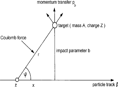
Figure 1: Kinematics of Coulomb scattering of a particle of charge $z$ on a target of charge $Z$

The Coulomb force between the incoming particle and the target is written as

$$\vec{F}=\frac{z\cdot e\cdot Z\cdot e}{r^{2}}\frac{\vec{r}}{r}\quad.$$ (10)

For symmetry reasons the net momentum transfer is only perpendicular to $\vec{p}$ along the impact parameter $b$

$$p_{b}=\int^{+\infty}_{-\infty}F_{b}{\rm d}t=\int^{+\infty}_{-\infty}\frac{z\cdot Z\cdot e^{2}}{r^{2}}\cdot\frac{b}{r}\cdot\frac{{\rm d}x}{\beta c}\quad,$$ (11)

with $b=r\sin\varphi$, d$t={\rm d}x/v={\rm d}x/\beta c$, and $F_{b}$ force perpendicular to $p$.

$$p_{b} = \frac{z\cdot Z\cdot e^{2}}{\beta c}\int^{+\infty}_{-\infty}\frac{b\,{\rm d}x}{(\sqrt{x^{2}+b^{2}})^{3}}=\frac{z\cdot Z\cdot e^{2}}{\beta cb}\underbrace{\int^{+\infty}_{-\infty}\frac{{\rm d}(x/b)}{\left(\sqrt{1+\left(\frac{x}{b}\right)^{2}}\right)^{3}}}_{=2}$$ (12)

$$p_{b} = \frac{2z\cdot Z\cdot e^{2}}{\beta cb}=\frac{2r_{e}m_{e}c}{b\beta}z\cdot Z\quad,$$ (13)

where $r_{e}$ is the classical electron radius. This consideration leads to a scattering angle

$$\Theta=\frac{p_{b}}{p}=\frac{2z\cdot Z\cdot e^{2}}{\beta cb}\cdot\frac{1}{p}\quad.$$ (14)

The cross section for this process is given by the well-known Rutherford formula

$$\frac{{\rm d}\sigma}{{\rm d}\Omega}=\frac{z^{2}Z^{2}r^{2}_{e}}{4}\left(\frac{m_{e}c}{\beta p}\right)^{2}\frac{1}{\sin^{4}\Theta/2}\quad.$$ (15)

Multiple Scattering

From eq. 15 one can see that the average scattering angle $\langle\Theta\rangle$ is zero. To characterize the different degrees of scattering when a particle passes through an absorber one normally uses the so-called “average scattering angle” $\sqrt{\langle\Theta^{2}\rangle}$. The projected angular distribution of scattering angles in this sense leads to an average scattering angle of r:cgru:[6]

$$\sqrt{\langle\Theta^{2}\rangle}=\Theta_{\rm plane}=\frac{13.6\,{\rm MeV}}{\beta cp}z\cdot\sqrt{\frac{x}{X_{0}}}\left\{1+0.038\ln\left(\frac{x}{X_{0}}\right)\right\}$$ (16)

with $p$ in MeV/c and $x$ the thickness of the scattering medium measured in radiation lengths $X_{0}$ (see Bremsstrahlung). The average scattering angle in three dimensions is

$$\Theta_{\rm space}=\sqrt{2}\,\Theta_{\rm plane}=\sqrt{2}\,\Theta_{0}\quad.$$ (17)

The projected angular distribution of scattering angles can approximately be represented by a Gaussian

$$P(\Theta){\rm d}\Theta=\frac{1}{\sqrt{2\pi}\Theta_{0}}\exp\left\{-\frac{\Theta^{2}}{2\Theta^{2}_{0}}\right\}{\rm d}\Theta\quad.$$ (18)

Energy Loss of Charged Particles

Charged particles interact with a medium via electromagnetic interactions by the exchange of photons. If the range of photons is short, the absorption of virtual photons constituting the field of the charged particle gives rise to ionization of the material. If the medium is transparent Cherenkov radiation can be emitted above a certain threshold. But also sub-threshold emission of electromagnetic radiation can occur, if discontinuities of the dielectric constant of the material are present (transition radiation) r:cgru:[7] . The emission of real photons by decelerating a charged particle in a Coulomb field also constitutes an important energy loss (bremsstrahlung).

Ionization Energy-Loss

Bethe-Bloch Formula

This energy-loss mechanism represents the scattering of charged particles off atomic electrons, e.g.

$$\mu^{+}+\mbox{atom}\rightarrow\mu^{+}+\mbox{atom}^{+}+e^{-}\quad.$$ (19)

The momentum transfer to the electron is (see eq. 13)

$$p_{b}=\frac{2r_{e}m_{e}c}{b\beta}z\quad,$$

and the energy transfer in the classical approximation

$$\varepsilon=\frac{p_{b}^{2}}{2m_{e}}=\frac{2r_{e}^{2}m_{e}c^{2}}{b^{2}\beta^{2}}z^{2}\quad.$$ (20)

The interaction probability per (g/cm²), given the atomic cross-section $\sigma$, is

$$\phi({\rm g}^{-1}{\rm cm}^{2})=\frac{N}{A}\sigma[{\rm cm}^{2}/{\rm atom}]$$ (21)

where $N$ is Avogadro’s constant.

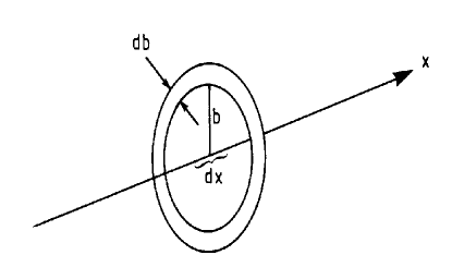
Figure 2: Sketch explaining the differential collision probability

The differential probability to hit an electron in the area of an annulus with radii $b$ and $b+{\rm d}b$ (see figure 2) with an energy transfer between $\varepsilon$ and $\varepsilon+{\rm d}\varepsilon$ is

$$\phi(\varepsilon){\rm d}\varepsilon=\frac{N}{A}2\pi b\,{\rm d}b\,Z\quad,$$ (22)

because there are $Z$ electrons per target atom.

Inserting $b$ from eq. 20 into eq. 22 gives

$$b^{2} = \frac{2r_{e}^{2}m_{e}c^{2}}{\beta^{2}}z^{2}\cdot\frac{1}{\varepsilon}$$

$$2|b\,{\rm d}b| = \frac{2r_{e}^{2}m_{e}c^{2}}{\beta^{2}}z^{2}\cdot\frac{{\rm d}\varepsilon}{\varepsilon^{2}}$$

$$\phi(\varepsilon){\rm d}\varepsilon = \frac{N}{A}\pi\frac{2r_{e}^{2}m_{e}c^{2}}{\beta^{2}}z^{2}\cdot Z\cdot\frac{{\rm d}\varepsilon}{\varepsilon^{2}}$$ (23)

$$= \frac{2\pi r_{e}^{2}m_{e}c^{2}N}{\beta^{2}}\cdot\frac{Z}{A}\cdot z^{2}\cdot\frac{{\rm d}\varepsilon}{\varepsilon^{2}}\quad,$$

showing that the energy spectrum of $\delta$-electrons or knock-on electrons follows an $1/\varepsilon^{2}$ dependence (figure 3, r:cgru:[8] ).

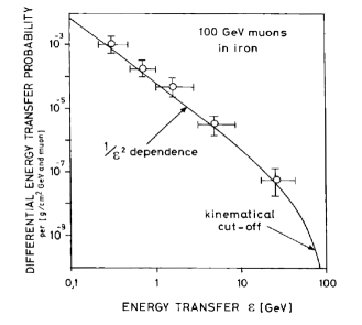
Figure 3: $1/\varepsilon^{2}$-dependence of the knock-on electron production probability r:cgru:[8]

The energy loss is now computed from eq. 22 by integrating over all possible impact parameters r:cgru:[5]

$$-{\rm d}E = \int^{\infty}_{0}\phi(\varepsilon)\cdot\varepsilon\cdot{\ d}x$$

$$= \int^{\infty}_{0}\frac{N}{A}2\pi b\cdot{\rm d}b\cdot Z\cdot\varepsilon\cdot{\rm d}x$$

$$-\frac{{\rm d}E}{{\rm d}x} = \frac{2\pi N}{A}\cdot Z\int^{\infty}_{0}\varepsilon\cdot b\cdot{\rm d}b$$ (24)

$$= 2\pi\frac{Z\cdot N}{A}\cdot\frac{2r_{e}^{2}m_{e}c^{2}}{\beta^{2}}z^{2}\int^{\infty}_{0}\frac{{\rm d}b}{b}\quad.$$

This classical calculation yields an integral which diverges for $b=0$ as well as for $b=\infty$. This is not a surprise because one would not expect that our approximations hold for these extremes.

• The $b=0$ case: Let us approximate the “size” of the target electron seen from the rest frame of the incident particle by half the de Broglie wavelength. This gives a minimum impact parameter of

  $$b_{\min}=\frac{h}{2p}=\frac{h}{2\gamma m_{e}\beta c}\quad.$$ (25)

• The $b=\infty$ case: If the revolution time $\tau_{R}$ of the electron in the target atom becomes smaller than the interaction time $\tau_{i}$, the incident particle “sees” a more or less neutral atom

  $$\tau_{i}=\frac{b_{\max}}{v}\sqrt{1-\beta^{2}}\quad.$$ (26)

The factor $\sqrt{1-\beta^{2}}$ takes into account that the field at high velocities is Lorentz-contracted. Hence the interaction time is shorter. For the revolution time we have

$$\tau_{R}=\frac{1}{\nu_{Z}\cdot Z}=\frac{h}{I}\quad,$$ (27)

where $I$ is the mean excitation energy of the target material, which can be approximated by

$$I=10eV\cdot Z$$ (28)

for elements heavier than sulphur.

The condition to see the target as neutral now leads to

$$\tau_{R}=\tau_{i}\qquad\Rightarrow\qquad\frac{b_{\max}}{v}\sqrt{1-\beta^{2}}=\frac{h}{I}$$

$$b_{\max}=\frac{\gamma h\beta c}{I}\quad.$$ (29)

With the help of eq. 25 and 29 we can solve the integral in eq. 24

$$-\frac{{\rm d}E}{{\rm d}x}=2\pi\cdot\frac{Z}{A}N\cdot\frac{2r_{e}^{2}m_{e}c^{2}}{\beta^{2}}z^{2}\cdot\ln\frac{2\gamma^{2}\beta^{2}m_{e}c^{2}}{I}\quad.$$ (30)

Since for long-distance interactions the Coulomb field is screened by the intervening matter one has

$$-\frac{{\rm d}E}{{\rm d}x}=\kappa z^{2}\cdot\frac{Z}{A}\frac{1}{\beta^{2}}\left[\ln\frac{2\gamma^{2}\beta^{2}m_{e}c^{2}}{I}-\eta\right]\quad,$$ (31)

where $\eta$ is a screening parameter (density parameter) and

$$\kappa=4\pi Nr^{2}_{e}m_{e}c^{2}\quad.$$

The exact treatment of the ionization energy loss of heavy particles leads to r:cgru:[6]

$$-\frac{{\rm d}E}{{\rm d}x}=\kappa z^{2}\cdot\frac{Z}{A}\cdot\frac{1}{\beta^{2}}\left[\frac{1}{2}\ln\frac{2m_{e}c^{2}\gamma^{2}\beta^{2}}{I^{2}}E_{\rm kin}^{\max}-\beta^{2}-\frac{\delta}{2}\right]$$ (32)

which reduces to eq. 31 for $\gamma m_{e}/m_{0}\ll 1$ and $\beta^{2}-\frac{\delta}{2}=\eta$.

The energy-loss rate of muons in iron is shown in Figure 4r:cgru:[6] . It exhibits a $\frac{1}{\beta^{2}}$-decrease until a minimum of ionization is obtained for $3\leq\beta\gamma\leq 4$.

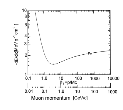
Figure 4: Energy loss of muons in iron r:cgru:[6]

Due to the $\ln\gamma$-term the energy loss increases again (relativistic rise, logarithmic rise) until a plateau is reached (density effect, Fermi plateau).

The energy loss is usually expressed in terms of the area density ${\rm d}s=\rho{\rm d}x$ with $\rho$-density of the absorber. It varies with the target material like $Z/A$ ($\leq 0.5$ for most elements). Minimum ionizing particles lose 1.94 MeV/(g/cm²) in helium decreasing to 1.08 MeV/(g/cm²) in uranium. The energy loss of minimum ionizing particles in hydrogen is exceptionally large, because here $Z/A=1$.

The relativistic rise saturates at high energies because the medium becomes polarized, effectively reducing the influence of distant collisions. The density correction $\delta/2$ can be described by

$$\frac{\delta}{2}=\ln\frac{\hbar\omega_{p}}{I}+\ln\beta\gamma-\frac{1}{2}$$ (33)

where

$$\hbar\omega_{p}=\sqrt{4\pi N_{e}r^{3}_{e}}m_{e}c^{2}/\alpha$$ (34)

is the plasma energy and $N_{e}$ the electron density of the absorbing material.

For gases the Fermi-plateau, which saturates the relativistic rise, is about $60\%$ higher compared to the minimum of ionization. Figure 5 shows the measured energy-loss rates of electrons, muons, pions, kaons, protons and deuterons in the PEP4/9-TPC (185 $dE/dx$ measurements at 8.5 atm in Ar-CH₄ = 80 : 20) r:cgru:[newNM] .

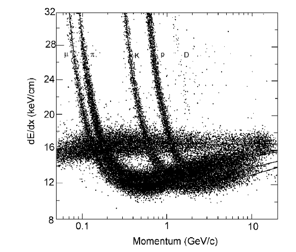
Figure 5: Measured ionization energy loss of electrons, muons, pions, kaons, protons and deuterons in the PEP4/9-TPC r:cgru:[newNM]

Landau Distributions

The Bethe-Bloch formula describes the average energy loss of charged particles. The fluctuation of the energy loss around the mean is described by an asymmetric distribution, the Landau distribution r:cgru:[10] ; r:cgru:[11] .

The probability $\phi(\varepsilon){\rm d}\varepsilon$ that a singly charged particle loses an energy between $\varepsilon$ and $\varepsilon+{\rm d}\varepsilon$ per unit length of an absorber was (eq. 23)

$$\phi(\varepsilon)=\frac{2\pi Ne^{4}}{m_{e}v^{2}}\frac{Z}{A}\cdot\frac{1}{\varepsilon^{2}}\quad.$$ (35)

Let us define

$$\xi=\frac{2\pi Ne^{4}}{m_{e}v^{2}}\cdot\frac{Z}{A}x\quad,$$ (36)

where $x$ is the area density of the absorber:

$$\phi(\varepsilon)=\xi(x)\frac{1}{x\varepsilon^{2}}\quad.$$ (37)

Numerically one can write

$$\xi=\frac{0.1536}{\beta^{2}}\frac{Z}{A}\cdot x\quad\mbox{[keV]}\quad,$$ (38)

where $x$ is measured in mg/cm².

For an absorber of 1 cm Ar we have for $\beta=1$

$$\xi=0.123\,{\rm keV}\quad.$$

We define now

$$f(x,\Delta)=\frac{1}{\xi}\omega(\lambda)$$ (39)

as the probability that the particle loses an energy $\Delta$ on traversing an absorber of thickness $x$. $\lambda$ is defined to be the normalized deviation from the most probable energy loss $\Delta^{\rm m.p.}$

$$\lambda=\frac{\Delta-\Delta^{\rm m.p.}}{\xi}\quad.$$ (40)

The most probable energy loss is calculated to be r:cgru:[10] ; r:cgru:[12]

$$\Delta^{\rm m.p.}=\xi\left\{\ln\frac{2m_{e}c^{2}\beta^{2}\gamma^{2}\xi}{I^{2}}-\beta^{2}+1-\gamma_{E}\right\}\quad,$$ (41)

where $\gamma_{E}=0.577\ldots$ is Euler’s constant.

Landau’s treatment of $f(x,\Delta)$ yields

$$\omega(\lambda)=\frac{1}{\pi}\int^{\infty}_{0}{\rm e}^{-u\ln u-\lambda u}\sin\pi u{\rm d}u\quad,$$ (42)

which can be approximated by r:cgru:[12]

$$\Omega(\lambda)=\frac{1}{\sqrt{2\pi}}\exp\left\{-\frac{1}{2}(\lambda+{\rm e}^{-\lambda})\right\}\quad.$$ (43)

Figure 6 shows the energy loss distribution of 3 GeV electrons in an Ar/CH₄ (80:20) filled drift chamber of 0.5 cm thickness r:cgru:[13] . According to equation 35 the $\delta$-ray contribution to the energy loss falls inversely proportional to the energy transfer squared, producing a long tail, called Landau tail, in the energy-loss distribution up to the kinematical limit (see also figure 3).

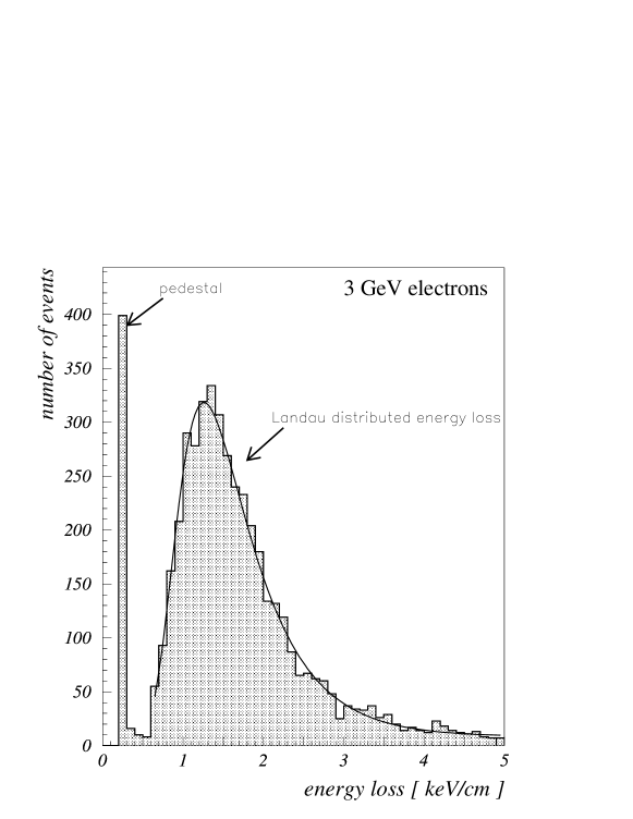
Figure 6: Energy-loss distribution of 3 GeV electrons in a thin-gap multiwire drift chamber r:cgru:[13]

The asymmetric property of the energy-loss distribution becomes obvious for thin absorbers. For larger absorber thicknesses or truncation techniques applied to thin absorbers the Landau distribution gets more symmetric.

Scintillation in Materials

Scintillator materials can be inorganic crystals, organic liquids or plastics and gases. The scintillation mechanism in organic crystals is an effect of the lattice. Incident particles can transfer energy to the lattice by creating electron-hole pairs or taking electrons to higher energy levels below the conduction band. Recombination of electron-hole pairs may lead to the emission of light. Also electron-hole bound states (excitons) moving through the lattice can emit light when hitting an activator center and transferring their binding energy to activator levels, which subsequently deexcite. In thallium doped NaI-crystals about 25 eV are required to produce one scintillation photon. The decay time in inorganic scintillators can be quite long (1$\mu$s in CsI (Tl); 0.62 $\mu$s in BaF₂).

In organic substances the scintillation mechanism is different. Certain types of molecules will release a small fraction ($\approx$ 3%) of the absorbed energy as optical photons. This process is expecially marked in organic substances which contain aromatic rings, such as polystyrene, polyvinyltoluene, and naphtalene. Liquids which scintillate include toluene or xylene r:cgru:[6] .

This primary scintillation light is preferentially emitted in the UV-range. The absorption length for UV-photons in the scintillation material is rather short: the scintillator is not transparent for its own scintillation light. Therefore, this light is transferred to a wavelength shifter which absorbs the UV-light and reemits it at longer wavelengths (e.g. in the green). Due to the lower concentration of the wavelength shifter material the reemitted light can get out of the scintillator and be detected by a photosensitive device. The technique of wavelength shifting is also used to match the emitted light to the spectral sensitivity of the photomultiplier. For plastic scintillators the primary scintillator and wavelength shifter are mixed with an organic material to form a polymerizing structure. In liquid scintillators the two active components are mixed with an organic base r:cgru:[2] .

About 100 eV are required to produce one photon in an organic scintillator. The decay time of the light signal in plastic scintillators is substantially shorter compared to inorganic substances (e.g. 30 ns in naphtalene).

Because of the low light absorption in gases there is no need for wavelength shifting in gas scintillators.

Plastic scintillators do not respond linearly to the energy-loss density. The number of photons produced by charged particles is described by Birk’s semi-empirical formula r:cgru:[6] ; r:cgru:[17] ; r:cgru:[18]

$$N=N_{0}\frac{{\rm d}E/{\rm d}x}{1+k_{B}\,{\rm d}E/{\rm d}x}\quad,$$ (44)

where $N_{0}$ is the photon yield at low specific ionization density, and $k_{B}$ is Birk’s density parameter. For 100 MeV protons in plastic scintillators one has d$E/$d$x\approx 10$ MeV/(g/cm²) and $k_{B}\approx 5$ mg/(cm²MeV), yielding a saturation effect of $\sim 5$% r:cgru:[4] .

For low energy losses eq. 44 leads to a linear dependence

$$N=N_{0}\cdot{\rm d}E/{\rm d}x\quad,$$ (45)

while for very high d$E/$d$x$ saturation occurs at

$$N=N_{0}/k_{B}\quad.$$ (46)

There exists a correlation between the energy loss of a particle that goes into the creation of electron-ion pairs or the production of scintillation light because electron-ion pairs can recombine thus reducing the d$E/$d$x|_{\rm ion}$-signal. On the other hand the scintillation light signal is enhanced because recombination frequently leads to excited states which deexcite yielding scintillation light.

Cherenkov Radiation

A charged particle traversing a medium with refractive index $n$ with a velocity $v$ exceeding the velocity of light $c/n$ in that medium, emits Cherenkov radiation. The threshold condition is given by

$$\beta_{\rm thres}=\frac{v_{\rm thres}}{c}\geq\frac{1}{n}\quad.$$ (47)

The angle of emission increases with the velocity reaching a maximum value for $\beta=1$, namely

$$\Theta_{c}^{\max}=\arccos\frac{1}{n}\quad.$$ (48)

The threshold velocity translates into a threshold energy

$$E_{\rm thres}=\gamma_{\rm thres}m_{0}c^{2}$$ (49)

yielding

$$\gamma_{\rm thres}=\frac{1}{\sqrt{1-\beta^{2}_{\rm thres}}}=\frac{n}{\sqrt{n^{2}-1}}\quad.$$ (50)

The number of Cherenkov photons emitted per unit path length d$x$ is

$$\frac{{\rm d}N}{{\rm d}x}=2\pi\alpha z^{2}\int\left(1-\frac{1}{n^{2}\beta^{2}}\right)\frac{{\rm d}\lambda}{\lambda^{2}}$$ (51)

for $n(\lambda)>1$, $z$ – electric charge of the incident particle, $\lambda$ – wavelength, and $\alpha$ – fine structure constant. The yield of Cherenkov radiation photons is proportional to $1/\lambda^{2}$, but only for those wavelengths where the refractive index is larger than unity. Since $n(\lambda)\approx 1$ in the X-ray region, there is no X-ray Cherenkov emission. Integrating eq. 51 over the visible spectrum ($\lambda_{1}=400$ nm, $\lambda_{2}=700$ nm) gives

$$\frac{{\rm d}N}{{\rm d}x} = 2\pi\alpha z^{2}\frac{\lambda_{2}-\lambda_{1}}{\lambda_{1}\lambda_{2}}\sin^{2}\Theta_{c}$$ (52)

$$= 490\cdot z^{2}\cdot\sin^{2}\Theta_{c}\,[{\rm cm}^{-1}]\quad.$$

The Cherenkov effect can be used to identify particles of fixed momentum by means of threshold Cherenkov counters. More information can be obtained, if the Cherenkov angle is measured by DIRC-counters (Detection of Internally Reflected Cherenkov light). In these devices some fraction of the Cherenkov light produced by a charged particle is kept inside the radiator by total internal reflection. The direction of the photons remains unchanged and the Cherenkov angle is conserved during the transport. When exiting the radiator the photons produce a Cherenkov ring on a planar detector (figure 7).

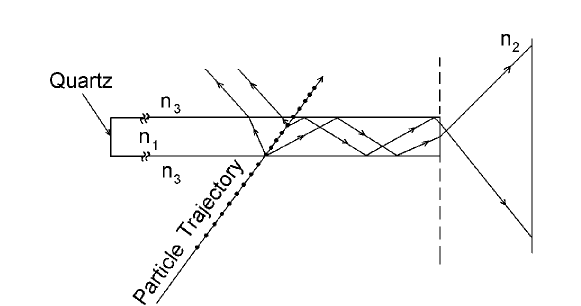
Figure 7: Imaging principle of a DIRC-counter r:cgru:Adam

The pion/proton separation achieved with such a system is shown in figure 8r:cgru:Adam .

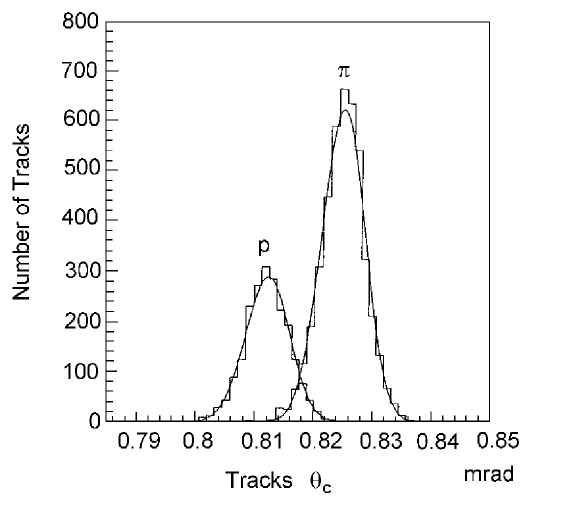
Figure 8: Cherenkov-angle distribution for pions and protons of 5.4 GeV/c in a DIRC-counter r:cgru:Adam .

Ring-imaging Cherenkov-counters (RICH-counters) have become extraordinary useful in the field of elementary particles and astrophysics. Figure 9 shows the Cherenkov ring radii of electrons, muons, pions and kaons in a C₄F₁₀-Ar (75:25) filled Rich-counter read out by a 100-channel photomultipiler of $10*10$ cm² active area r:cgru:Debbe .

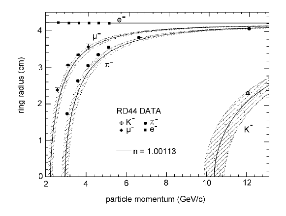
Figure 9: Cherenkov-ring radii of $e,\mu,\pi,K$ in a C₄F₁₀-Ar (75:25) RICH-counter. The solid curves show the expected radii for an index of refraction of n = 1.00113. The shaded regions represent a 5% uncertainty in the absolute momentum scale r:cgru:Debbe

Transition Radiation

Transition radiation is emitted when a charged particle traverses a medium with discontinuous dielectric constant. A charged particle moving towards a boundary, where the dielectric constant changes, can be considered to form together with its mirror charge an electric dipole whose field strength varies in time. The time dependent dipole field causes the emission of electromagnetic radiation. This emission can be understood in such a way that although the dielectric displacement $\vec{D}=\varepsilon\varepsilon_{0}\vec{E}$ varies continuously in passing through a boundary, the electric field does not.

The energy radiated from a single boundary (transition from vacuum to a medium with dielectric constant $\varepsilon$) is proportional to the Lorentz-factor of the incident charged particle r:cgru:[6] ; r:cgru:[17] ; r:cgru:[21] :

$$S=\frac{1}{3}\alpha z^{2}\hbar\omega_{p}\gamma\quad,$$ (53)

where $\hbar\omega_{p}$ is the plasma energy (see equation 34). For commonly used plastic radiators (styrene or similar materials) one has

$$\hbar\omega_{p}\approx 20\,{\rm eV}\quad.$$ (54)

The typical emission angle of transition radiation is proportional to $1/\gamma$. The radiation yield drops sharply for frequencies

$$\omega>\gamma\omega_{p}\quad.$$ (55)

The $\gamma$-dependence of the emitted energy originates mainly from the hardening of the spectrum rather than from the increased photon yield. Since the radiated photons also have energies proportional to the Lorentz factor of the incident particle, the number of emitted transition radiation photons is

$$N\propto\alpha z^{2}\quad.$$ (56)

The number of emitted photons can be increased by using many transitions (stack of foils, or foam). At each interface the emission probability for an X-ray photon is of the order of $\alpha=1/137$. However, the foils or foams have to be of low $Z$ material to avoid absorption in the radiator. Interference effects for radiation from transitions in periodic arrangements cause an effective threshold behaviour at a value of $\gamma\approx 1000$. These effects also produce a frequency dependent photon yield. The foil thickness must be comparable to or larger than the formation zone

$$D=\gamma c/\omega_{p}$$ (57)

which in practical situations ($\hbar\omega_{p}=20\,$eV; $\gamma=5\cdot 10^{3}$) is about 50 $\mu$m. Transition radiation detectors are mainly used for $e/\pi$-setaration. In cosmic ray experiments transition radiation emission can also be employed to measure the energy of muons in the TeV-range.

Bremsstrahlung

If a charged particle is decelerated in the Coulomb field of a nucleus a fraction of its kinetic energy will be emitted in form of real photons (bremsstrahlung). The energy loss by bremsstrahlung for high energies can be described by r:cgru:[2]

$$-\frac{{\rm d}E}{{\rm d}x}=4\alpha N_{A}\frac{Z^{2}}{A}\cdot z^{2}r^{2}E\ln\frac{183}{Z^{1/3}}\quad,$$ (58)

where $r=\frac{1}{4\pi\varepsilon_{0}}\cdot\frac{e^{2}}{mc^{2}}$. Bremsstrahlung is mainly produced by electrons because

$$r_{e}\propto\frac{1}{m_{e}}\quad.$$ (59)

Equation 58 can be rewritten for electrons

$$-\frac{{\rm d}E}{{\rm d}x}=\frac{E}{X_{0}}\quad,$$ (60)

where

$$X_{0}=\frac{A}{4\alpha N_{A}Z(Z+1)r_{e}^{2}\ln(183\,Z^{-1/3})}$$ (61)

is the radiation length of the absorber in which bremsstrahlung is produced. Here we have included also radiation from electrons ($\sim Z$, because there are $Z$ electrons per nucleus). If screening effects are taken into account $X_{0}$ can be more accurately described by r:cgru:[6]

$$X_{0}=\frac{716.4\,A}{Z(Z+1)\ln(287/\sqrt{Z})}\quad[{\rm g/cm}^{2}]\quad.$$ (62)

The important point about bremsstrahlung is that the energy loss is proportional to the energy. The energy where the losses due to ionization and bremsstrahlung for electrons are the same is called critical energy

$$\left.\frac{{\rm d}E_{c}}{{\rm d}x}\right|_{\rm ion}=\left.\frac{{\rm d}E_{c}}{{\rm d}x}\right|_{\rm brems}\quad.$$ (63)

For solid or liquid absorbers the critical energy can be approximated by r:cgru:[6]

$$E_{c}=\frac{610\,{\rm MeV}}{Z+1.24}\quad,$$ (64)

while for gases one has r:cgru:[6]

$$E_{c}=\frac{710\,{\rm MeV}}{Z+0.92}\quad.$$ (65)

The difference between gases on the one hand and solids and liquids on the other hand comes about because the density corrections are different in these substances, and this modifies $\left.\frac{{\rm d}E}{{\rm d}x}\right|_{\rm ion}$.

The energy spectrum of bremsstrahlung photons is $\sim E_{\gamma}^{-1}$, where $E_{\gamma}$ is the photon energy.

At high energies also radiation from heavier particles becomes important and consequently a critical energy for these particles can be defined. Since

$$\left.\frac{{\rm d}E}{{\rm d}x}\right|_{\rm brems}\propto\frac{1}{{\rm m}^{2}}$$ (66)

the critical energy e.g. for muons in iron is

$$E_{c}=\frac{610\,{\rm MeV}}{Z+1.24}\cdot\left(\frac{m_{\mu}}{m_{e}}\right)^{2}=960\,{\rm GeV}\quad.$$ (67)

Direct Electron Pair Production

Direct electron pair production in the Coulomb field of a nucleus via virtual photons (“tridents”) is a dominant energy loss mechanism at high energies. The energy loss for singly charged particles due to this process can be represented by

$$\left.-\frac{{\rm d}E}{{\rm d}x}\right|_{\rm pair}=b(Z,A,E)\cdot E\quad.$$ (68)

It is essentially - like bremsstrahlung - also proportional to the particle’s energy. Because bremsstrahlung and direct pair production dominate at high energies this offers an attractive possibility to build also muon calorimeters r:cgru:[2] . The average rate of muon energy losses can be parametrized as

$$\frac{{\rm d}E}{{\rm d}x}=a(E)+b(E)\cdot E$$ (69)

where $a(E)$ represents the ionization energy loss and $b(E)$ is the sum of direct elektron pair production, bremsstrahlung and photonuclear interactions.

The various contributions to the energy loss of muons in standard rock (Z = 11; A = 22; $\rho=3g/cm^{3}$) are shown in figure 10.

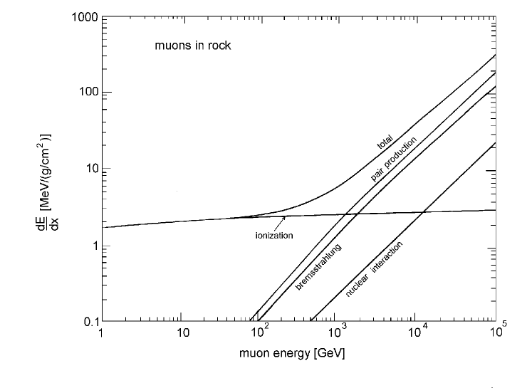
Figure 10: Contributions to the energy loss of muons in standard rock (Z = 11; A = 22; $\rho=3g/cm^{3}$).

Nuclear Interactions

Nuclear interactions play an important role in the detection of neutral particles other than photons. They are also responsible for the development of hadronic cascades. The total cross section for nucleons is of the order of 50 mbarn and varies slightly with energy. It has an elastic ($\sigma_{\rm el}$) and inelastic part ($\sigma_{\rm inel}$). The inelastic cross section has a material dependence

$$\sigma_{\rm inel}\approx\sigma_{0}A^{\alpha}$$ (70)

with $\alpha=0.71$. The corresponding absorption length $\lambda_{a}$ is r:cgru:[2]

$$\lambda_{a}=\frac{A}{N_{A}\cdot\rho\cdot\sigma_{\rm inel}}[{\rm cm}]$$ (71)

($A$ in g/mol, $N_{A}$ in mol^-1, $\rho$ in g/cm³, and $\sigma_{\rm inel}$ in cm²).
This quantity has to be distinguished from the nuclear interaction length $\lambda_{w}$, which is related to the total cross section

$$\lambda_{w}=\frac{A}{N_{A}\cdot\rho\cdot\sigma_{\rm total}}[{\rm cm}]\quad.$$ (72)

Since $\sigma_{\rm total}>\sigma_{\rm inel}$, $\lambda_{w}<\lambda_{a}$ holds.

Strong interactions have a multiplicity which grows logarithmically with energy. The particles are produced in a narrow cone around the forward direction with an average transverse momentum of $p_{T}=350\,$MeV/c, which is responsible for the lateral spread of hadronic cascades.

A useful relation for the calculation of interaction rates per (g/cm²) is

$$\phi(({\rm g/cm}^{2})^{-1})=\sigma_{N}\cdot N_{A}$$ (73)

where $\sigma_{N}$ is the cross section per nucleon and $N_{A}$ Avogadro’s number.

Interaction of Photons

Photons are attenuated in matter via the processes of the photoelectric effect, Compton scattering and pair production. The intensity of a photon beam varies in matter according to

$$I=I_{0}\>{\rm e}^{-\mu x}\quad,$$ (74)

where $\mu$ is mass attenuation coefficient. $\mu$ is related to the photon cross sections $\sigma_{i}$ by

$$\mu=\frac{N_{A}}{A}\sum^{3}_{i=1}\sigma_{i}\quad.$$ (75)

Photoelectric Effect

Atomic electrons can absorb the energy of a photon completely

$$\gamma+\mbox{atom}\rightarrow\mbox{atom}^{+}+e^{-}\quad.$$ (76)

The cross section for absorption of a photon of energy $E_{\gamma}$ is particularly large in the $K$-shell (80% of the total cross section). The total cross section for photon absorption in the $K$-shell is

$$\sigma^{K}_{\rm Photo}=\left(\frac{32}{\varepsilon^{7}}\right)^{1/2}\alpha^{4}Z^{5}\sigma_{\rm Thomson}[{\rm cm}^{2}/{\rm atom}]\quad,$$ (77)

where $\varepsilon=E_{\gamma}/m_{e}c^{2}$, and $\sigma_{\rm Thomson}=\frac{8}{3}\pi r_{e}^{2}=665$ mbarn is the cross section for Thomson scattering. For high energies the energy dependence becomes softer

$$\sigma^{K}_{\rm Photo}=4\pi r_{e}^{2}Z^{5}\alpha^{4}\cdot\frac{1}{\varepsilon}\quad.$$ (78)

The photoelectric cross section has sharp discontinuities when $E_{\gamma}$ coincides with the binding energy of atomic shells. As a consequence of a photoabsorption in the $K$-shell characteristic X-rays or Auger electrons are emitted r:cgru:[2] .

Compton Scattering

The Compton effect describes the scattering of photons off quasi-free atomic electrons

$$\gamma+e\rightarrow\gamma^{\prime}+e^{\prime}\quad.$$ (79)

The cross section for this process, given by the Klein-Nishina formula, can be approximated at high energies by

$$\sigma_{c}\propto\frac{\ln\varepsilon}{\varepsilon}\cdot Z$$ (80)

where $Z$ is the number of electrons in the target atom. From energy and momentum conservation one can derive the ratio of scattered ($E_{\gamma}^{\prime}$) to incident photon energy ($E_{\gamma}$)

$$\frac{E_{\gamma}^{\prime}}{E_{\gamma}}=\frac{1}{1+\varepsilon(1-\cos\Theta_{\gamma})}\quad,$$ (81)

where $\Theta_{\gamma}$ is the scattering angle of the photon with respect to its original direction.

For backscattering ($\Theta_{\gamma}=\pi$) the energy transfer to the electron $E_{\rm kin}$ reaches a maximum value

$$E^{\max}_{\rm kin}=\frac{2\varepsilon^{2}}{1+2\varepsilon}m_{e}c^{2}\quad,$$ (82)

which, in the extreme case ($\varepsilon\gg 1$), equals $E_{\gamma}$.

In Compton scattering only a fraction of the photon energy is transferred to the electron. Therefore, one defines an energy scattering cross section

$$\sigma_{cs}=\frac{E_{\gamma}^{\prime}}{E_{\gamma}}\sigma_{c}$$ (83)

and an energy absorption cross section

$$\sigma_{ca}=\sigma_{c}-\sigma_{cs}=\sigma_{c}\frac{E_{\rm kin}}{E_{\gamma}}\quad.$$ (84)

At accelerators and in astrophysics also the process of inverse Compton scattering is of importance r:cgru:[2] .

Pair Production

The production of an electron-positron pair in the Coulomb field of a nucleus requires a certain minimum energy

$$E_{\gamma}\geq 2m_{e}c^{2}+\frac{2m_{e}^{2}c^{2}}{m_{\rm nucleus}}\quad.$$ (85)

Since for all practical cases $m_{\rm nucleus}\gg m_{e}$, one has effectively $E_{\gamma}\geq 2m_{e}c^{2}$.

The total cross section in the case of complete screening $\left(\varepsilon\gg\frac{1}{\alpha Z^{1/3}}\right)$; i.e. at reasonably high energies $(E_{\gamma}\gg 20\,$MeV), is

$$\sigma_{\rm pair}=4\alpha r^{2}_{e}Z^{2}\left(\frac{7}{9}\ln\frac{183}{Z^{1/3}}-\frac{1}{54}\right)\quad[{\rm cm}^{2}/{\rm atom}]\quad.$$ (86)

Neglecting the small additive term $1/54$ in eq. 86 one can rewrite, using eq. 58 and eq. 61,

$$\sigma_{\rm pair}=\frac{7}{9}\frac{A}{N_{A}}\cdot\frac{1}{X_{0}}\quad.$$ (87)

The partition of the energy to the electron and positron is symmetric at low energies $(E_{\gamma}\ll 50\,$MeV) and increasingly asymmetric at high energies $(E_{\gamma}>1\,$GeV) r:cgru:[2] .

Figure 11 shows the photoproduction of an electron-positron pair in the Coulomb-field of an electron ($\gamma+e^{-}\rightarrow e^{+}+e^{-}+e^{-}$) and also a pair-production in the field of a nucleus ($\gamma+\mbox{nucleus}\rightarrow e^{+}+e^{-}+\mbox{nucleus}^{\prime}$) r:cgru:Close .

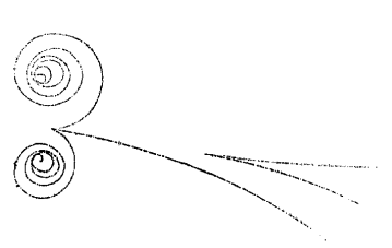
Figure 11: Photoproduction in the Coulomb-field of an electron ($\gamma+e^{-}\rightarrow e^{+}+e^{-}+e^{-}$) and on a nucleus ($\gamma+\mbox{nucleus}\rightarrow e^{+}+e^{-}+\mbox{nucleus}^{\prime}$) r:cgru:Close

Mass-Attenuation Coefficients

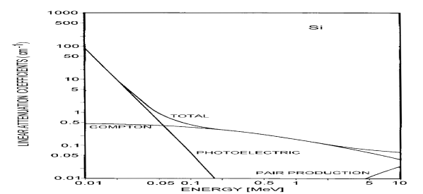
Figure 12: Mass attenuation coefficients for photon interactions in silicon r:cgru:[30]

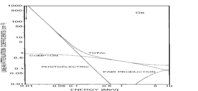
Figure 13: Mass attenuation coefficients for photon interactions in germanium r:cgru:[30]

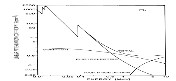
Figure 14: Mass attenuation coefficients for photon interactions in lead r:cgru:[30]

The mass-attenuation coefficients for photon interactions are shown in figures 14-14 for silicon, germanium and lead r:cgru:[30] . The photoelectric effect dominates at low energies ($E_{\gamma}<100\,$keV). Superimposed on the continuous photoelectric attenuation coefficient are absorption edges characteristic of the absorber material. Pair production dominates at high energies ($>10$ MeV). In the intermediate region Compton scattering prevails.

Interaction of Neutrons

In the same way as photons are detected via their interactions also neutrons have to be measured indirectly. Depending on the neutron energy various reactions can be considered which produce charged particles which are then detected via their ionization or scintillation r:cgru:[2] .

• Low energies ($<20\,$MeV)

  $$n+{{}^{6}{\rm Li}} \rightarrow \alpha+{{}^{3}{\rm H}}$$

  $$n+{{}^{10}{\rm B}} \rightarrow \alpha+{{}^{7}{\rm Li}}$$

  $$n+{{}^{3}{\rm He}} \rightarrow p+{{}^{3}{\rm H}}$$ (88)

  $$n+p \rightarrow n+p$$

  The conversion material can be a component of a scintillator (e.g. LiI (Tl)), a thin layer of material in front of the sensitive volume of a gaseous detector (boron layer), or an admixture to the counting gas of a proportional counter (BF₃, ³He, or protons in CH₄).

• Medium energies ($20\,{\rm MeV}\leq E_{\rm kin}\leq 1\,$GeV)
  The ($n,p$)-recoil reaction can be used for neutron detection in detectors which contain many quasi-free protons in their sensitive volume (e.g. hydrocarbons).

• High energies ($E>1\,$GeV)
  Neutrons of high energy initiate hadron cascades in inelastic interactions which are easy to identify in hadron calorimeters.

Neutrons are detected with relatively high efficiency at very low energies. Therefore, it is often useful to slow down neutrons with substances containing many protons, because neutrons can transfer a large amount of energy to collision partners of the same mass. In some fields of application, like in radiation protection at nuclear reactors, it is of importance to know the energy of fission neutrons, because the relative biological effectiveness depends on it. This can e.g. be achieved with a stack of plastic detectors interleaved with foils of materials with different threshold energies for neutron conversion r:cgru:[28] .

Interactions of Neutrinos

Neutrinos are very difficult to detect. Depending on the neutrino flavor the following inverse beta decay like interactions can be considered:

$$\nu_{e}+n \rightarrow p+e^{-}$$

$$\bar{\nu}_{e}+p \rightarrow n+e^{+}\vspace{1mm}$$

$$\nu_{\mu}+n \rightarrow p+\mu^{-}$$

$$\bar{\nu}_{\mu}+p \rightarrow n+\mu^{+}\vspace{1mm}$$ (89)

$$\nu_{\tau}+n \rightarrow p+\tau^{-}$$

$$\bar{\nu}_{\tau}+p \rightarrow n+\tau^{+}$$

The cross section for $\nu_{e}$-detection in the MeV-range can be estimated as r:cgru:[32]

$$\sigma(\nu_{e}N) = \frac{4}{\pi}\cdot 10^{-10}\left(\frac{\hbar p}{(m_{p}c)^{2}}\right)^{2}$$ (90)

$$= 6.4\cdot 10^{-44}{\rm cm}^{2}\mbox{ for 1\,MeV}\quad.$$

This means that the interaction probability of e.g. solar neutrinos in a water Cherenkov counter of $d=100$ meter thickness is only

$$\phi=\sigma\cdot N_{A}\cdot d=3.8\cdot 10^{-16}\quad.$$ (91)

Since the coupling constant of weak interactions has a dimension of 1/GeV², the neutrino cross section must rise at high energies like the square of the center-of-mass energy. For fixed target experiments we can parametrize

$$\sigma(\nu_{\mu}N) = 0.67\cdot 10^{-38}E_{\nu}[{\rm GeV}]\quad{\rm cm}^{2}/{\rm nucleon}$$

$$\sigma(\bar{\nu}_{\mu}N) = 0.34\cdot 10^{-38}E_{\nu}[{\rm GeV}]\quad{\rm cm}^{2}/{\rm nucleon}$$ (92)

This shows that even at 100 GeV the neutrino cross section is lower by 11 orders of magnitude compared to the total proton-proton cross section.

Electromagnetic Cascades

The development of cascades induced by electrons, positrons or photons is governed by bremsstrahlung of electrons and pair production of photons. Secondary particle production continues until photons fall below the pair production threshold, and energy losses of electrons other than bremsstrahlung start to dominate: the number of shower particles decays exponentially.

Already a very simple model can describe the main features of particle multiplication in electromagnetic cascades: A photon of energy $E_{0}$ starts the cascade by producing an $e^{+}e^{-}$-pair after one radiation length. Assuming that the energy is shared symmetrically between the particles at each multiplication step, one gets at the depth $t$

$$N(t)=2^{t}$$ (93)

particles with energy

$$E(t)=E_{0}\cdot 2^{-t}\quad.$$ (94)

The multiplication continues until the electrons fall below the critical energy $E_{c}$

$$E_{c}=E_{0}\cdot 2^{-t_{\max}}\quad.$$ (95)

From then on ($t>t_{\max}$) the shower particles are only absorbed. The position of the shower maximum is obtained from eq. 95

$$t_{\max}=\frac{\ln E_{0}/E_{c}}{\ln 2}\propto\ln E_{0}\quad.$$ (96)

The total number of shower particles is

$$S = \sum^{t_{\max}}_{t=0}N(t)=\sum 2^{t}=2^{t_{\max}+1}-1\approx 2^{t_{\max}+1}$$

$$S = 2\cdot 2^{t_{\max}}=2\cdot\frac{E_{0}}{E_{c}}\propto E_{0}\quad.$$ (97)

If the shower particles are sampled in steps $t$ measured in units of $X_{0}$, the total track length is obtained as

$$S^{\ast}=\frac{S}{t}=2\frac{E_{0}}{E_{c}}\cdot\frac{1}{t}\quad,$$ (98)

which leads to an energy resolution of

$$\frac{\sigma}{E_{0}}=\frac{\sqrt{S^{\ast}}}{S^{\ast}}=\frac{\sqrt{t}}{\sqrt{2E_{0}/E_{c}}}\propto\frac{\sqrt{t}}{\sqrt{E_{0}}}\quad.$$ (99)

In a more realistic description the longitudinal development of the electron shower can be approximated by r:cgru:[6]

$$\frac{{\rm d}E}{{\rm d}t}=\mbox{const}\cdot t^{a}\cdot{\rm e}^{-bt}\quad,$$ (100)

where $a$, $b$ are fit parameters.

Figure 15 shows muon induced electromagnetic cascades in a multi-plate cloud chamber r:cgru:[new34] .

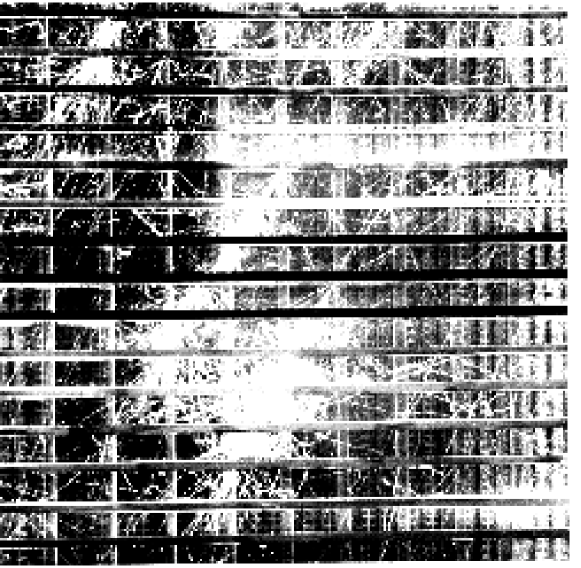
Figure 15: Some muon induced electromagnetic cascades in a multi-plate cloud chamber operated in a concrete shielded air shower array r:cgru:[new34]

The lateral spread of an electromagnetic shower is mainly caused by multiple scattering. It is described by the Molière radius

$$R_{m}=\frac{21\,{\rm MeV}}{E_{c}}X_{0}\>[{\rm g/cm}^{2}]\quad.$$ (101)

95% of the shower energy in a homogeneous calorimeter is contained in a cylinder of radius $2R_{m}$ around the shower axis.

Figure 16 demonstrates the interplay of the longitudinal and lateral development of an electromagnetic shower r:cgru:[2] .

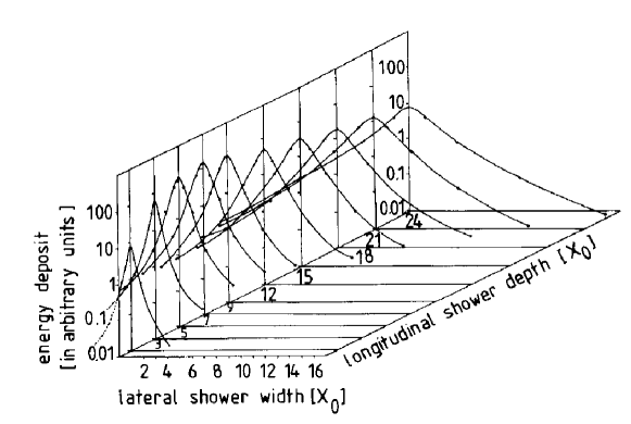
Figure 16: Sketch of the longitudinal and lateral development of an electromagnetic cascade in a homogeneous absorber r:cgru:[2]

Hadron Cascades

The longitudinal development of electromagnetic cascades is characterized by the radiation length $X_{0}$ and their lateral width is determined by multiple scattering. In contrast to this, hadron showers are governed in their longitudinal structure by the nuclear interaction length $\lambda$ and by transverse momenta of secondary particles as far as lateral width is concerned. Since for most materials $\lambda\gg X_{0}$, and $\langle p_{T}^{\rm interaction}\rangle\gg\langle p_{T}^{\rm multiple\>scattering}\rangle$ hadron showers are longer and wider.

Part of the energy of the incident hadron is spent to break up nuclear bonds. This fraction of the energy is invisible in hadron calorimeters. Further energy is lost by escaping particles like neutrinos and muons as a result of hadron decays. Since the fraction of lost binding energy and escaping particles fluctuates considerably, the energy resolution of hadron calorimeters is systematically inferior to electron calorimeters.

The longitudinal development of pion induced hadron cascades is plotted in figure 17. Figure 18 shows a comparison between proton, iron, and photon induced cascades in the atmosphere r:cgru:knapp .

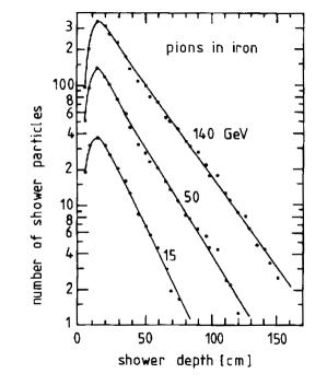
Figure 17: Longitudinal development of pion induced hadron cascades r:cgru:[37]

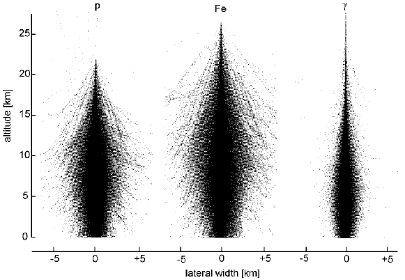
Figure 18: Comparison between proton, iron, and photon induced cascades in the atmosphere. The primary energy in each case is 10¹⁴eV r:cgru:knapp .

The different response of calorimeters to electrons and hadrons is an undesirable feature for the energy measurement of jets of unknown particle composition. By appropriate compensation techniques, however, the electron to hadron response can be equalized.

Particle Identification

Particle identification is based on measurements which are sensitive to the particle velocity, its charge and its momentum. Figure 19 sketches the different possibilities to separate photons, electrons, positrons, muons, charged pions, protons, neutrons and neutrinos in a mixed particle beam using a general purpose detector.

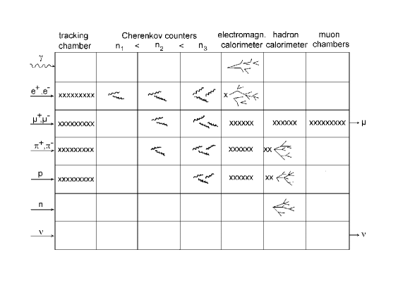
Figure 19: Particle identification using a detector consisting of a tracking chamber, Cherenkov counters, calorimetry and muon chambers.

Figure 20 shows the particle separation power of a balloon borne experiment using momentum, time-of-flight, dE/dx and Cherenkov radiation measurements r:cgru:Mitchell .

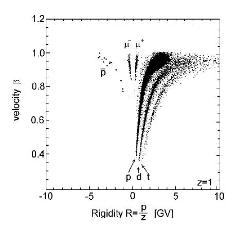
Figure 20: Particle identification in a balloon borne experiment using momentum, time-of-flight, dE/dx and Cherenkov radiation information r:cgru:Mitchell .

Even the abundance of different helium isotopes can be determined from a velocity and momentum measurement (figure 21 r:cgru:Simon ). This is feasable, because at fixed momentum the lighter isotope ³He is faster than the more abundant ⁴He.

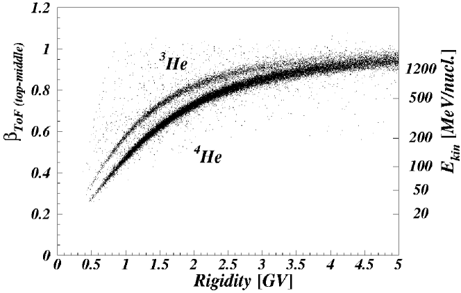
Figure 21: Isotopic abundance of energetic cosmic ray helium nuclei r:cgru:Simon

Conclusion

Basic physical principles can be used to identify all kinds of elementary particles and nuclei. The precise measurement of the particle composition in high energy physics experiments at accelerators and in cosmic rays is essential for the insight into the underlying physics processes. This is an important ingredient for the progress in the fields of elementary particles and astrophysics aiming at the unification of forces and the understanding of the evolution of the universe.

References

- (1) K. Kleinknecht, Detectors for Particle Radiation , Cambridge University Press 1998
- (2) C. Grupen, Particle Detectors , Cambridge University Press 1996
- (3) R. Fernow, Introduction to Experimental Particle Physics , Cambridge University Press 1989
- (4) W.R. Leo, Techniques for Nuclear and Particle Physics Experiments , Springer, Berlin 1987
- (5) B. Rossi, High Energy Particles , Prentice-Hall (1952)
- (6) Particle Data Group, R.M. Barnett et al., Phys.Rev. D54 (1996) 1; Eur. Phys. J. C3 (1998) 1
-
(7)
W.W.M. Allison, P.R.S. Wright, Oxford Univ. Preprint 35/83
(1983) and
W.W.M. Allison, J.H. Cobb, Ann.Rev.Nucl.Sci. 30 (1980) 253 - (8) C. Grupen, Ph.D. Thesis, University of Kiel 1970
- (9) D. R. Nygren, J. N. Marx, Physics Today 31 (1978) 46
- (10) D.H. Wilkinson, Nucl.Instr.Meth. A 383 (1996) 513
- (11) L.D. Landau, J.Exp.Phys. (USSR) 8 (1944) 201
- (12) S. Behrens, A.C. Melissinos, Univ. of Rochester Preprint UR-776 (1981)
- (13) K. Affholderbach et al., Nucl. Instr. Meth. A 410 (1998) 166
- (14) R.C. Fernow, Brookhaven Nat.Lab. Preprint BNL-42114 (1988)
- (15) J. Birks, Theory and Practice of Scintillation Counting , MacMillan 1964
- (16) I. Adam et al. SLAC-Pub-7706, Nov. 1997; and hep-ex/9712001
- (17) R. Debbe et al. hep-ex/9503006 (1995)
- (18) S. Paul, CERN-PPE 91-199 (1991)
- (19) F. Close, M. Marten, C. Sutton, The Particle Explosion, Oxford University Press 1987
- (20) Harshaw Chemical Company (H. Lentz, L. van Gelderen, Th. Courbois) 1969
- (21) E. Sauter, Grundlagen des Strahlenschutzes , Thiemig, München 1982
- (22) D.H. Perkins Introduction to High Energy Physics , Addison-Wesley, 1986
- (23) W. Wolter, private communication 1999
- (24) J. Knapp, D. Heck Luftschauer-Simulationsrechnungen mit dem Corsika-Programm Forschungszentrum Karlsruhe Nachrichten 30 (1998) 27
- (25) M. Holder et al., Nucl.Instr.Meth. 151 69 (1978)
- (26) J. W. Mitchell et al. Phys. Rev. Lett. 76 (1996) 3057
- (27) M. Simon, H. Göbel, private communication 1999