Identifying nonlinear wave interactions in plasmas
using two-point measurements:
A case study of Short Large Amplitude
Magnetic Structures (SLAMS)

Abstract

Two fundamental quantities for characterizing nonlinear wave phenomena in plasmas are the spectral energy transfer associated with the energy redistribution between Fourier modes, and the linear growth rate. It is shown how these quantities can be estimated simultaneously from dual-spacecraft data using Volterra series models. We consider magnetic field data gathered upstream the Earth’s quasiparallel bow shock, in which Short Large Amplitude Magnetic Structures (SLAMS) supposedly play a leading role. The analysis attests the dynamic evolution of the SLAMS and reveals an energy cascade toward high-frequency waves. These results put constraints on possible mechanisms for the shock front formation.

1 Introduction

In this paper, a Volterra series representation is used to describe the nonlinear evolution in time and in space of a fluctuating wave field. The basis for this approach is that plasmas can often be viewed as a causal nonlinear system (a “black box”) that reacts to a given excitation by giving a response. By modeling the nonlinear transfer function associated with this system, deeper insight can be gained into the underlying physics.

The analysis of the nonlinear transfer function is detailed here for the particular case where two-point measurements are available. First, we show how to model the dynamical response. Then, the physical interpretation of the model coefficients is given. Particular attention is paid to the linear growth rate, which expresses the linear instability of the wave field, and to the spectral energy transfer, which describes how the instabilities saturate through nonlinear wave interactions.

We apply this method to magnetic field data gathered by the dual AMPTE satellites near the Earth’s quasiparallel bow shock. This data set corresponds to a regime of quasi-stationary turbulence in a collisionless plasma; it has received much interest in relation with the existence of Short Large Amplitude Magnetic Structures (SLAMS) [Schwartz et al., 1992]. It is shown how a transfer function analysis reveals the role played by these nonlinear structures.

This paper is divided in three parts. The experimental context is described in section 2. Sections 3 to 7 are devoted to data analysis aspects with a description of the model, the choice of its parameters, and its validation. Finally, in sections 8 and 9, experimental data are analyzed and interpreted.

2 The Experimental Context

The magnetic field data of interest were gathered by the dual Active Magnetospheric Particle Tracer Explorers spacecraft (United Kingdom Satellite (AMPTE-UKS) and Ion Release Module (AMPTE-IRM)) on day 304 of 1984 just upstream the Earth’s quasi-parallel bow shock. Several studies have already been devoted to this particular event [Schwartz and Burgess, 1991, Schwartz et al., 1992; Mann et al., 1994; Dudok de Wit and Krasnosel’skikh, 1995; Dudok de Wit et al., 1995], which provides a paradigm for nonlinear effects in turbulence. The spacecraft were closely following each other on the same outbound orbit (with a separation of $\delta x=144$ km), depicted in Figure 1.

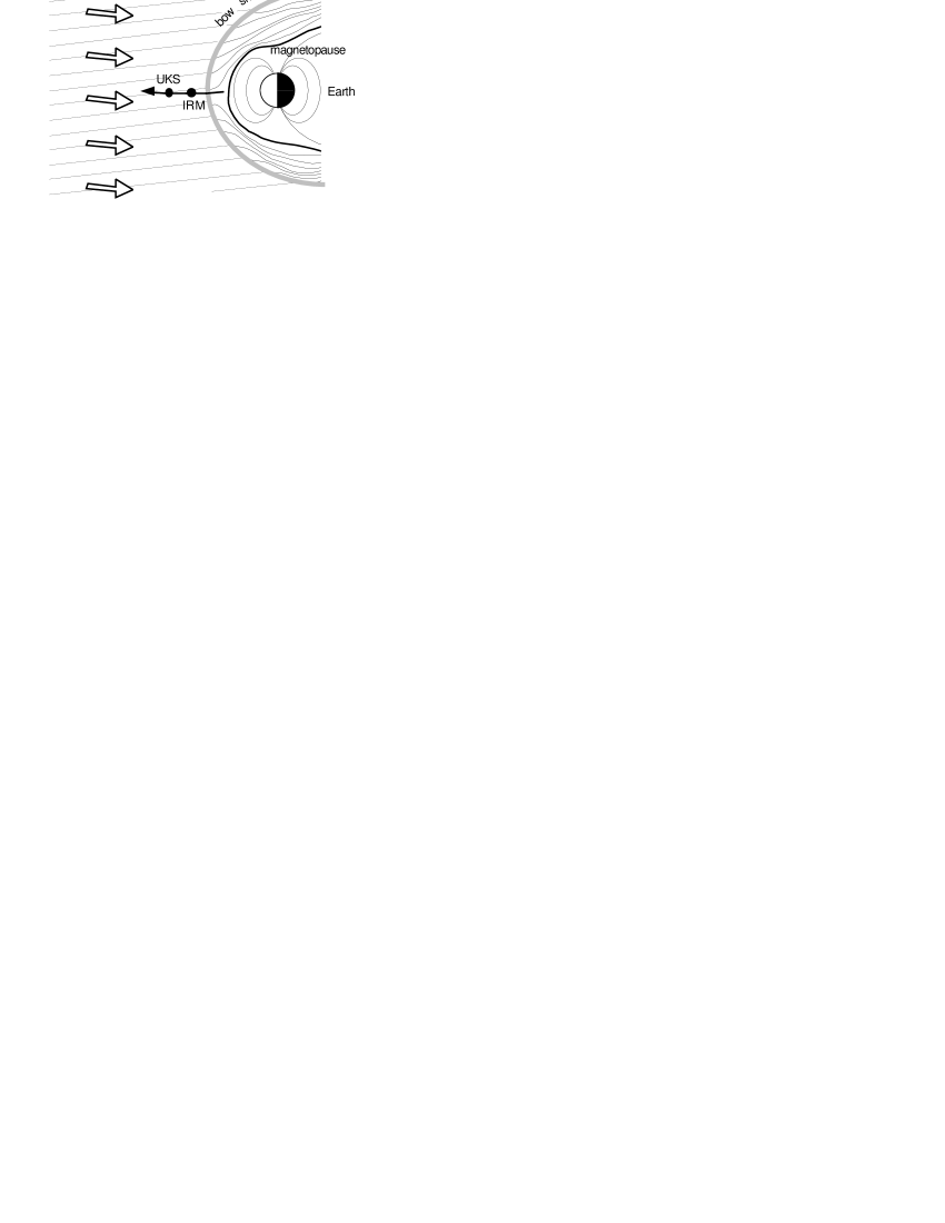
Figure 1: Configuration of the Earth’s bow shock showing the magnetic field lines, the orientation of the solar wind, and the orbit of the spacecraft for the event considered in this paper.

A distinctive feature of the studied region is the occurrence of SLAMS, which supposedly play a leading role in the shock front formation [Schwartz et al., 1992]. The shock wave is caused by the sudden deceleration of the supersonic solar wind at the encounter of the Earth’s magnetosphere. The SLAMS grow out of low-frequency waves that propagate away from the shock front but are convected back toward the Earth by the solar wind [Thomsen et al., 1990]. This steepening process is likely to result from an interaction with ion beams coming from the shock front [Scholer, 1993].

There are several open questions regarding the role played by SLAMS. Quasi-parallel shocks are currently viewed either as an entity [Winske et al., 1990] or as a patchy transition zone made by a merging of SLAMS [Schwartz and Burgess, 1991]. The relationship between the SLAMS and the whistler wave packets that frequently occur at their leading edge is not well understood either, although there is numerical [Omidi and Winske, 1990] and experimental [Dudok de Wit and Krasnosel’skikh, 1995] evidence for a causal link between the two.

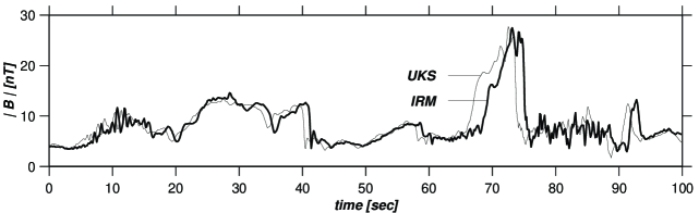
Figure 2: Excerpt of the time evolution of the magnetic field amplitude, as measured by the two spacecraft. A typical SLAMS appears at $t=$71 s. The precursor whistler wave appears at its trailing edge since the wave field is convected backward by the strong solar wind.

An excerpt of the magnetometer data is shown in Figure 2. The trajectory of the spacecraft, the prevailing magnetic field and the average solar wind velocity ($v_{sw}=$ 370 km/s) are all parallel within a few degrees. This is an important point since it means that both spacecraft see the same structures, separated by a time interval of about 1 s. A comparative analysis should therefore reveal how the wave field, and in particular the SLAMS, evolve as they move from one spacecraft to the other. We do this by building a Volterra model that tries to predict the wave field of AMPTE-IRM using the data of AMPTE-UKS as input.

Each spacecraft provides a data set which consists of the three components of the magnetic field, measured immediately upstream the shock front. For each component the number of samples is $4521$; the data were sampled at a constant rate of 8 Hz after being low-pass filtered at 4 Hz. We have chosen to consider the three components as different ensembles, thereby artificially increasing the sample size by a factor of 3. The anisotropy of the wave field a priori does not justify such an approximation, but no significant differences were found between the model coefficients as estimated separately from each component. An obvious future extension would be to have a model that takes into account the vectorial nature of the wave field.

The power spectral density of the wave field is illustrated in Figure 3a and can be qualified as being continuous and essentially featureless. Notice that all frequencies are expressed in the spacecraft reference frame, in which they are Doppler-shifted by the strong solar wind. The spectral densities are almost the same for the two spacecraft. Figure 3b shows the wave field probability distribution, which has non-Gaussian tails. The departure from Gaussianity should be underlined, since it is a necessary condition for having nonlinear wave-wave interactions [Kim and Powers, 1979].

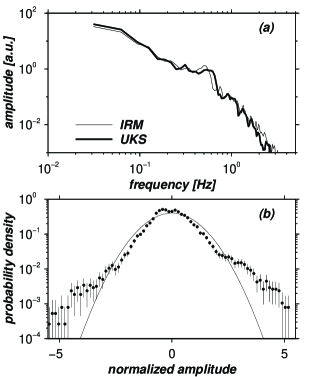
Figure 3: (a) Power spectral density and (b) probability distribution of the magnetic field of AMPTE-UKS projected along the direction of maximum variance. The solid line corresponds to a Gaussian distribution with the same variance; all amplitudes are normalized to have unit variance.

3 Modeling the Nonlinear Transfer Function

Much work has been done on the theory of nonlinear transfer functions in turbulence [e.g., Monin and Yaglom, 1975; Krommes, 1997] but relatively little is known about their inference from experimental data, which can be an unwieldy task. Early results were obtained in the context of neutral fluid turbulence [Uberoi, 1963; Van Atta and Chen, 1969; Lii et al., 1982; Ritz et al., 1988a] and later in plasmas [Ritz and Powers, 1986; Ritz et al., 1988b; Ritz et al., 1989; Kim et al., 1996]. Powers, Ritz and their coworkers contributed to the development of a computational framework for two-point measurements [Ritz and Powers, 1986; Ritz et al., 1989], thereby rendering the technique easily accessible to a large class of experiments. Their results, however, have remained overlooked, presumably because of the apparent computational investment and the difficulty in validating estimates that are prone to errors. In this paper we show how to increase the robustness of the estimates by using continuous wavelet transforms instead of the usual Fourier transform.

3.1 Volterra Series

Consider a stationary wave field which is measured in time and in space, and let $y(x,t)$ denote fluctuations around a fixed value. We are interested in describing the dynamics of this wave field with the following general model:

$$\frac{\partial{y(x,t)}}{\partial x}=F\big{(}y(x,t)\big{)}\ ,$$ (1)

where $F(y)$ is a continuous, nonlinear and time-invariant operator. Wiener [1958] showed that for a large class of causal systems $F(y)$ can be expanded as a Volterra (or Volterra-Fréchet-Wiener) series [Schetzen, 1980], which we write here after taking the Fourier transform of the time variable

$$\frac{\partial{y(x,\omega)}}{\partial x}=\Gamma(\omega)\>y(x,\omega)$$

$$+ \int\Gamma(\omega_{1},\omega_{2})\>y(x,\omega_{1})\>y(x,\omega_{2})$$

$$\hskip 19.91692pt\times\ \delta(\omega_{1}+\omega_{2}-\omega)\;d\omega_{1}d\omega_{2}$$

$$+ \int\!\!\!\int\Gamma(\omega_{1},\omega_{2},\omega_{3})\>y(x,\omega_{1})\>y(x,\omega_{2})$$

$$\hskip 19.91692pt\times\ y(x,\omega_{3})\>\delta(\omega_{1}+\omega_{2}+\omega_{3}-\omega)\>d\omega_{1}d\omega_{2}d\omega_{3}$$

$$+ \cdots$$

The kernels $\Gamma$ are directly related to the higher-order spectra of the process and have a physical meaning. $\Gamma(\omega)$, $\Gamma(\omega_{1},\omega_{2})$, and $\Gamma(\omega_{1},\omega_{2},\omega_{3})$ are respectively called the linear, quadratic, and cubic interaction terms. The generic situation corresponds to a leading linear term, which describes the linear dynamics of the system, such as the linear growth rate and the dispersion. The quadratic term expresses three-wave processes in which interactions occur within triads of waves that satisfy the resonance condition

$$\omega=\omega_{1}+\omega_{2}\ .$$ (3)

The cubic term similarly describes four-wave processes whose frequencies satisfy the selection rules

$$\omega=\omega_{1}+\omega_{2}+\omega_{3}\ \ \mbox{\rm or}\ \ \omega+\omega_{1}=\omega_{2}+\omega_{3}\ .$$ (4)

The main motivation for using a Volterra series expansion stems from its ability to describe various weakly nonlinear processes in plasmas [Kadomtsev, 1982], ranging from generic drift wave turbulence [Balk et al., 1990; Horton and Hasegawa, 1994] to Langmuir turbulence as described by the Zakharov equations [Musher et al., 1995]. Particular attention has been given to Hamiltonian systems [Zakharov et al., 1985] in which the kernels can be calculated explicitly. The resonant interactions defined by (3) and (4) are further known to be the building elements of turbulence as observed in collisionless plasmas: the decay and modulational instabilities, for example, are adequately described in terms of three-wave and four-wave interactions [Krasnosel’skikh and Lefeuvre, 1993].

Theoretical and experimental considerations show that for weak turbulence the low-order Volterra kernels are the predominant ones. Indeed, the characteristic timescale associated with the action of a $q$th-order kernel increases with $q$, making low-order kernels much more likely to rule the dynamics [Zakharov et al., 1985]. In practice, (3.1) may thus safely be truncated after the cubic term and quite often even a quadratically nonlinear model suffices.

3.2 Strong Versus Weak Turbulence

The nonlinear model of (3.1) formally applies to weak turbulence only, in which the dispersion and the characteristic growth rates of the Fourier modes are small. Solar wind turbulence, on the other hand, is often considered as being of the strong turbulence type. The region we study is actually a mixture between the two since the dynamical properties of the wave field are dominated by a small population of energetic ions interacting with a plasma of the weak turbulence type. The weakness of the dispersion [Dudok de Wit et al.,, 1995] and the relatively small value of the linear growth rate (see Section 8) support the validity of the weak turbulence approximation here.

The extension from weak to strong turbulence as a first approximation implies a loosening of the resonance conditions (equations (3)-(5)) to account for the finite bandwidth of the wave packets [Horton and Hasegawa, 1994]. We shall take this spectral broadening implicitly into account by projecting the wave field on wavelets instead of Fourier modes (see Section 5).

3.3 Spatial Versus Temporal Description

Equation (3.1) is actually a particular case of a class of models that describe both the spatial and the temporal structure of the wave field. In a more general setting, both wavenumbers and frequencies must satisfy resonance conditions. Energy and momentum conservation force three-wave interactions to occur along the resonant manifold

$$\omega({\mathbf{k}}_{1}+{\mathbf{k}}_{2})=\omega_{1}({\mathbf{k}}_{1})+\omega_{2}({\mathbf{k}}_{2})\ ,$$ (5)

where ${\mathbf{k}}$ denotes the wave-number vector.

The wavenumber dependence of the interaction is often omitted by lack of spatially resolved experiments. It raises an important point, which is the separation between spatial and temporal scales, and the distinction between stationarity and homogeneity. In our experiment, the wave field is convected past the satellites by the solar wind and so the angular frequency $\omega_{sat}$ we observe in the spacecraft frame is in fact Doppler-shifted, giving, $\omega_{sat}=\omega_{pl}+{\mathbf{k}}\cdot{\mathbf{v}}_{sw}$. However, because the wavenumber ${\mathbf{k}}$ and the solar wind velocity ${\mathbf{v}}_{sw}$ are almost parallel, and because of the fast solar wind, we may approximate $\omega_{sat}\approx\omega_{pl}+k\,v_{sw}\approx k\,v_{sw}$. This expression suggests that the spatial structure of the wave field, projected on the solar wind velocity vector, can be probed simply by measuring the time evolution and viceversa. This approximation is known as the Taylor hypothesis and allows us to exchange temporal dynamics and spatial structure

$$\frac{\partial y}{\partial t}\longleftrightarrow v_{sw}\frac{\partial y}{\partial x}\ .$$ (6)

There now remains to convert the Eulerian representation of the experiment into a Lagrangian one, in which the magnetic structures are followed from one spacecraft to the other. A space-time representation of the spacecraft (see Figure 4) indeed reveals that by taking the difference of the spacecraft signals, we mix the wave field time derivative and the spatial gradient. A Galilean transformation is needed $y(x,t)\rightarrow y(x,t^{\prime}=t-x/v_{sw})$, which we do by shifting the AMPTE-IRM time series by $\tau=-\delta x/v_{sw}=-0.39$ s. An additional correction of $-0.28$ s is needed to compensate for differences in timing conventions [see Schwartz et al., 1992].

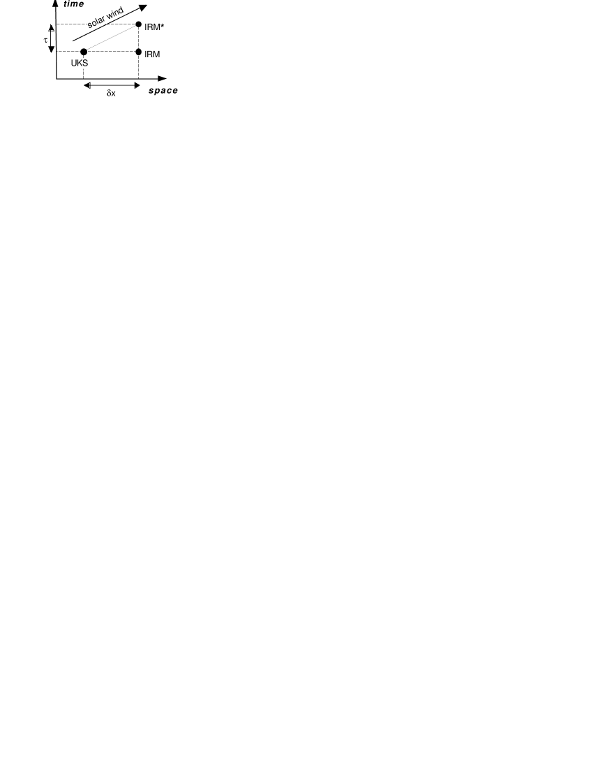
Figure 4: Representation of the spacecraft in space-time, showing the correspondence between spatial separation $\delta x$ and time delay $\tau$. The actual position of IRM must be moved to IRM^∗ to compensate for the effect of the solar wind.

3.4 Inferring the Model Coefficients

Physical insight into our model can be gained by introducing the real-valued density of waves $E(\omega,x)$, by analogy to the number of quasi particles in condensed matter theory. For a large ensemble of waves with different frequencies, the random-phase approximation holds, giving

$$\langle y(\omega_{1},x)y^{*}(\omega_{2},x)\rangle=E(\omega_{1},x)\delta(\omega_{1}-\omega_{2})\ .$$ (7)

Angle brackets denote ensemble-averaging, which is often replaced by time averaging, assuming ergodicity. From equations (3.1) and (7) we obtain the kinetic equation

$$\frac{\partial{E(\omega,x)}}{\partial t}=2\overline{\gamma}(\omega)E(\omega,x)$$

$$+ 2\>\int\!\!\int T(\omega_{1},\omega_{2})\;\delta(\omega_{1}+\omega_{2}-\omega)\;d\omega_{1}\>d\omega_{2}$$

$$+ \cdots$$

which models the nonlinear evolution taking place between the two spacecraft. Notice that we used the Taylor hypothesis (equation (6)) to interchange spatial and temporal derivatives. The quantities of interest are the average linear growth rate in time

$$\overline{\gamma}(\omega)=v_{sw}\>{\mathrm{R}e}\left[\Gamma(\omega)\right]$$ (9)

and the average quadratic energy transfer rate

$$T(\omega_{1},\omega_{2})=v_{sw}\>{\mathrm{R}e}\left[\>\Gamma(\omega_{1},\omega_{2})\right.$$

$$\times \left.\langle y(\omega_{1},x)\>y(\omega_{2},x)\>y^{*}(\omega_{1}+\omega_{2},x)\rangle\>\right]\ .$$

The latter attests the existence of non local interactions which are a hallmark of nonlinearity. Equation (3.4) shows that the energy flux in Fourier space $\partial{E}/\partial{t}$ results from a balance between energy dissipation (or gain) at a given frequency $\omega$ and spectral energy transfers between $\omega$ and other frequencies.

Nonlinear transfer functions have the advantage of revealing both the magnitude and the orientation of spectral energy fluxes: positive values of $T(\omega_{1},\omega_{2})$ correspond to three-wave interactions in which spectral components with angular frequencies $\omega_{1}>0$ and $\omega_{2}>0$ transfer energy to the component $\omega=\omega_{1}+\omega_{2}$. We shall write this as $\omega_{1}+\omega_{2}\rightarrow\omega$. Conversely, negative values correspond to decay processes $\omega\rightarrow\omega_{1}+\omega_{2}$.

There is a close resemblance between the definition of the energy transfer function (equation (3.4)) and that of the auto bispectrum [Mendel, 1991],

$$B(\omega_{1},\omega_{2})=\langle y(\omega_{1},x)\>y(\omega_{2},x)\>y^{*}(\omega_{1}+\omega_{2},x)\rangle\ ,$$ (11)

which has been widely used for quantifying quadratic wave interactions in plasmas [Kim and Powers, 1979; Lagoutte et al., 1989; LaBelle and Lund, 1992; Pécseli et al., 1993; Dudok de Wit and Krasnosel’skikh, 1995; Bale et al., 1996]. Transfer functions, however, are more informative since they detect the presence of nonlinear interactions between the observation points irrespective of what happened farther upstream. Consider for example a wave field that underwent nonlinear interactions during its early history but is now fully static. This wave field will have a nonzero cross-bispectrum even though nonlinear interactions aren’t actually taking place. A nonzero bispectrum thus does not necessarily attest the existence of wave-wave interactions at the observation point. Such a caveat was put forward in an analytic example by Pécseli and Trulsen [1993]. The energy transfer function on the contrary detects whether energy is being exchanged between spectral modes, causing the amplitudes and the phases to vary locally in time and in space. This new information can be accessed only by comparing the wave field as it goes from one observation point to the other. Finally, we note that the existence of energy transfers presupposes a weak nonstationarity or inhomogeneity of the wave field.

3.5 Symmetries

The real-valued nature of the data and the definition of the transfer function automatically give rise to a number of symmetry relations, which shrink the principal domain in frequency space, significantly reducing the number of model coefficients to be computed [see Nam and Powers, 1994]. The principal domain of the energy transfer function is even smaller, since for $\omega_{1}+\omega_{2}=\omega$ we have

$$T(\omega_{1},\omega_{2})=T(\omega_{2},\omega_{1})=-T(\omega,-\omega_{1})=-T(\omega,-\omega_{2})\ .$$ (12)

4 Estimating the Nonlinear Transfer Function

Our principal problem is the robust estimation of Volterra kernels from finite and noise-corrupted data. This problem may be alleviated by assuming a Gaussian probability distribution of the wave field, since the different regressors can then be identified separately. This assumption, however, rarely holds in practice. Incidentally, it is precisely the nonlinearity that causes the distribution to depart from Gaussianity. We therefore follow a more general procedure along the line developed by Ritz and Powers [1986] and later improved by Kim and Powers, [1988].

For discrete values of the frequency and with two-point measurements, (3.1) becomes

$$\frac{y_{\omega}(x\!+\!\delta x)-y_{\omega}(x)}{\delta x} = \Gamma_{\omega}\>y_{\omega}(x)$$

$$+ \frac{1}{2}\!\!\!\sum_{\mathop{{}_{\omega_{1},\omega_{2}}}\limits_{\omega=\omega_{1}+\omega_{2}}}\!\!\!\Lambda_{\omega_{1},\omega_{2}}^{\omega}\>y_{\omega_{1}}(x)\>y_{\omega_{2}}(x)$$

$$+ \cdots$$

where $y_{\omega}(x)$ is the discrete Fourier transform of $y(x,t)$ and $\{\omega\}=\{\omega_{1},\omega_{2},\cdots,\omega_{N_{\omega}}\}$ are the regularly spaced frequencies. Without loss of generality we assume that the ensemble average vanishes $\langle y(x,t)\rangle=0$. It is convenient to express the complex wave field $y_{\omega}(x)$ as

$$y_{\omega}(x)=|y_{\omega}(x)|e^{j\phi_{\omega}(x)}\ .$$ (14)

From (4) and (14) and in the limit where $\delta x\rightarrow 0$, we obtain a new system [Ritz and Powers, 1986]

$$Y_{\omega}=L_{\omega}U_{\omega}+\frac{1}{2}\sum_{\mathop{{}_{\omega_{1},\omega_{2}}}\limits_{\omega=\omega_{1}+\omega_{2}}}Q_{\omega_{1},\omega_{2}}^{\omega}U_{\omega_{1}}U_{\omega_{2}}+\cdots$$ (15)

with

$$Y_{\omega} = y_{\omega}(x+\delta x)$$ (16)

$$U_{\omega} = y_{\omega}(x)$$

$$L_{\omega} = (\Gamma_{\omega}\delta t+1-j\>\delta\phi_{\omega})\;e^{j\>\delta\phi_{\omega}}$$

$$Q_{\omega_{1},\omega_{2}}^{\omega} = \Lambda_{\omega_{1},\omega_{2}}^{\omega}\>\delta t\>e^{j\>\delta\phi_{\omega}}$$

$$\delta t = \delta x/v_{sw}$$

$$\delta\phi_{\omega} = \phi_{\omega}(x+\delta x)-\phi_{\omega}(x)\ .$$

From this system, the physical quantities $\Gamma_{\omega}$ and $\Lambda_{\omega_{1},\omega_{2}}^{\omega}$ can be computed directly, as shown by Ritz et al. [1989].

Equation (15) formally represents a nonlinear transfer function that links an output $Y_{\omega}$ (the waveform of AMPTE-IRM) to an input $U_{\omega}$ (the waveform of AMPTE-UKS). The estimation of the linear part of such a transfer function is a central problem in system identification, for which well-established techniques exist [Ljung, 1987; Priestley, 1981]. Comparatively few experimental efforts, however, have been directed toward the robust estimation of quadratic and higher-order transfer functions [Tick, 1961; Brillinger, 1970; Billings, 1980; Bendat, 1990]. For the sake of simplicity, we shall henceforth restrict ourselves to quadratically nonlinear models.

The simplest solution consists in selecting the model whose coefficients minimize the squared residual errors $\varepsilon_{\omega}$ between the measured wave field and the predicted one ${\hat{Y}}_{\omega}$

$$\varepsilon_{\omega}=|Y_{\omega}-{\hat{Y}}_{\omega}|^{2}\ .$$ (17)

The problem then reduces to a multiple linear regression with a unique solution. For each angular frequency $\omega$ we solve for ${\mathsf{H}}_{\omega}$,

$${\mathsf{U}}_{\omega}{\mathsf{H}}_{\omega}={\mathsf{Y}}_{\omega}\ ,$$ (18)

with

$${\mathsf{U}}_{\omega} = \left[\begin{array}[]{cccc}U_{\omega}(1)&U_{\omega_{1}}(1)\;U_{\omega-\omega_{1}}(1)&U_{\omega_{2}}(1)\;U_{\omega-\omega_{2}}(1)&\\ U_{\omega}(2)&U_{\omega_{1}}(2)\;U_{\omega-\omega_{1}}(2)&U_{\omega_{2}}(2)\;U_{\omega-\omega_{2}}(2)&\cdots\\ \vdots&\vdots&\vdots&\\ U_{\omega}(N_{ens})&U_{\omega_{1}}(N_{ens})\;U_{\omega-\omega 1}(N_{ens})&U_{\omega_{2}}(N_{ens})\;U_{\omega-\omega_{2}}(N_{ens})&\end{array}\right]\ \ \ \ \ (19)$$

$${\mathsf{H}}_{\omega} = \left[L_{\omega},Q_{\omega_{1},\omega-\omega_{1}}^{\omega},Q_{\omega_{2},\omega-\omega_{2}}^{\omega},\cdots\right]^{T}$$

$${\mathsf{Y}}_{\omega} = \left[Y_{\omega}(1),Y_{\omega}(2),\cdots,Y_{\omega}(N_{ens})\right]^{T}\ .$$

Numbers refer to different ensembles collected under identical conditions, ${\footnotesize T}$ denotes transposition and the number of unknown coefficients is $N_{c}$. The conceptual simplicity of this approach and its straightforward generalization to cubic and higher-order interactions are clear advantages.

The nonlinear transfer function can be obtained by solving the overdetermined set of equations (equation (18)) using conventional least squares techniques but deeper insight can be gained by multiplying these equations on the left by ${\mathsf{U}}_{\omega}^{*}$, giving

$$\left[\begin{tabular}[]{c|c}$\langle|U_{\omega}|^{2}\rangle$&$\langle U_{\omega}^{*}\>U_{\omega^{\prime}}\>U_{\omega-\omega^{\prime}}\rangle$\\ \\ \hline\cr\\ $\langle U_{\omega}\>U_{\omega^{\prime}}^{*}\>U_{\omega-\omega^{\prime}}^{*}\rangle$&$\;\;\langle U_{\omega^{\prime}}^{*}\>U_{\omega-\omega^{\prime}}^{*}\>U_{\omega^{\prime\prime}}\>U_{\omega-\omega^{\prime\prime}}\rangle$\\ \end{tabular}\right]{\mathsf{H}}_{\omega}=\left[\begin{array}[]{c}\langle U_{\omega}^{*}\>Y_{\omega}\rangle\\ \langle U_{\omega^{\prime}}^{*}\>U_{\omega-\omega^{\prime}}^{*}\>Y_{\omega}\rangle\\ \langle U_{\omega^{\prime\prime}}^{*}\>U_{\omega-\omega^{\prime\prime}}^{*}\>Y_{\omega}\rangle\\ \vdots\end{array}\right]\ .\ \ \ \ \ (20)$$

The leading matrix (also called higher-order autocovariance matrix) can be divided into four blocks, one with a second order moment (the power spectral density), two with third-order moments (the bispectra) and one with fourth-order moments. The fact that moments of various orders are needed to properly estimate the linear properties of the wave field recalls the well-known closure problem which is ubiquitous in the spectral modelling of turbulence. Equation (20) also shows how the non-Gaussian nature of the wave field enters the results. If the wave field were Gaussian, then the off-diagonal blocks of the higher-order autocovariance matrix would vanish and a separate estimation of the different Volterra kernels would be possible.

5 Wavelet Versus Fourier Transform

For the solution of (20) to be numerically stable and physically relevant, it is essential to have $N_{ens}\gg N_{c}$ ($N_{c}$ is the number of unknown coefficients) and ${\mathsf{U}}_{\omega}$ nonsingular. A compromise is thus needed between $N_{ens}$ and the number of different Fourier modes $N_{\omega}$, hereafter referred to as the mesh resolution. Usually, time series are divided into (possibly overlapping) sequences, each of which is Fourier transformed. A better compromise can be achieved with wavelets, which offer additional resolution in time at the expense of a lower frequency resolution. The continuous wavelet transform of $y(t)$ is defined as

$$y(a,\tau)=\int y(t)\frac{1}{\sqrt{a}}\>h^{*}\left(\frac{t-\tau}{a}\right)\>dt\ ,$$ (21)

where $h(t)$ is the analyzing wavelet and $a$ its scale. The optimum tradeoff between time and frequency resolution is achieved with Gaussian or Morlet wavelets

$$h(t)=\frac{1}{\pi^{1/4}\>\sigma^{1/2}}e^{2\pi jt}\;e^{-t^{2}/2\sigma^{2}}\ ,$$ (22)

for which each scale is related to an instantaneous angular frequency $\omega=2\pi/a$. The frequency resolution, defined in terms of the cutoff frequency at 3 dB is $\Delta\omega/\omega=1/4\sigma$ and the usual Fourier transform is recovered for $\sigma\rightarrow\infty$.

Compared to windowed Fourier transforms, the wavelet transforms yield statistically better behaved estimates of the spectral properties [van Milligen et al., 1995; Dudok de Wit and Krasnosel’skikh, 1995]. Our motivation, however, is not just computational but also stems from the ability of wavelets to resolve transient and soliton-like features [Farge et al., 1996]. Indeed, the strongly turbulent magnetic field shows transient structures that are more akin to wavelets than to coherent waves with an infinite extension.

The main drawback of this approach is its greater computational burden, since the number of ensembles $N_{ens}$ now almost equals the number of samples. Furthermore, we are left with a free parameter, the wavelet width $\sigma$. Since a fixed mesh resolution is wanted, with no spectral overlap between adjacent components $Y_{\omega_{j}}$ and $Y_{\omega_{j+1}}$, we adapt the wavelet width to the frequency in order to have $\sigma\geq\omega/4\delta\omega$. An additional condition $\sigma\geq 1$ is imposed to prevent the analyzing wavelet from being too much distorted.

6 Validation Criteria for the Transfer Function Model

Validation is a key issue in Volterra model identification. There exists no single satisfactory criterion for performing such a validation, but to a large extent we can rely on well-established techniques that have been developed for linear systems [Ljung, 1987].

Since our problem involves the solution of a linear system of equations, a good starting point is an inspection of the degree of independence between the columns of the matrix ${\mathsf{U}}_{\omega}$ (equation (19)) and the output ${\mathsf{Y}}_{\omega}$. The correlation function between ${\mathsf{Y}}_{\omega}$ and the first column of ${\mathsf{U}}_{\omega}$

$$\gamma_{L}^{2}(\omega)=\frac{|\langle Y_{\omega}U_{\omega}^{*}\rangle|^{2}}{\langle|Y_{\omega}|^{2}\rangle\langle|U_{\omega}|^{2}\rangle}$$ (23)

indicates how well the linear transfer function succeeds in predicting the output. This is the coherence function, which is bounded between 0 and 1. Likewise, the correlation function between the output and other columns of the matrix gives

$$\gamma_{Q}^{2}(\omega_{1},\omega_{2})=\frac{|\langle Y_{\omega_{1}+\omega_{2}}U_{\omega_{1}}^{*}U_{\omega_{2}}^{*}\rangle|^{2}}{\langle|Y_{\omega_{1}+\omega_{2}}|^{2}\rangle\langle|U_{\omega_{1}}U_{\omega_{2}}|^{2}\rangle}\ .$$ (24)

This is the cross-bicoherence, i.e., the cross-bispectrum normalized to the power spectral density. Its value is bounded between zero for uncorrelated waves and unity for triads of waves whose phases are totally correlated. For a cubic model, one similarly defines the cross-tricoherence, which quantifies the strength of four-wave interactions

$$\gamma_{C}^{2}(\omega_{1},\omega_{2},\omega_{3})=\frac{|\langle Y_{\omega_{1}+\omega_{2}+\omega_{3}}U_{\omega_{1}}^{*}U_{\omega_{2}}^{*}U_{\omega_{3}}^{*}\rangle|^{2}}{\langle|Y_{\omega_{1}+\omega_{2}+\omega_{3}}|^{2}\rangle\langle|U_{\omega_{1}}U_{\omega_{2}}U_{\omega_{3}}|^{2}\rangle}\ .$$ (25)

Note that there exist variants of these definitions [e.g. Kravtchenko-Berejnoi et al., 1995].

Higher-order coherence functions reveal which spectral components are likely to be involved in nonlinear interactions. They do not, however, tells us whether the model is actually good in predicting the wave field. A high bicoherence, for example, does not yet justify the choice of a quadratically nonlinear model. A more global figure of merit is obtained by comparing the measured output signal $Y_{\omega}$ to the model prediction $\hat{Y}_{\omega}$

$$\gamma_{Y\hat{Y}}^{2}(\omega)=\frac{|\langle Y_{\omega}\hat{Y}_{\omega}^{*}\rangle|^{2}}{\langle|Y_{\omega}|^{2}\rangle\langle|\hat{Y}_{\omega}|^{2}\rangle}\ .$$ (26)

In practice, one half of the data is used to estimate the transfer function while the other half is kept for cross-validation. These simple prescription tools can be complemented by tests on the residuals, etc.

7 Choosing the Right Model

The choice of the model parameters involves three main issues. More specific aspects are deferred to the appendix.

7.1 Choice of the Model Order

The basic question of the model order should ideally be answered by computing Volterra kernels for various orders and truncating the series as soon as they become negligible. The finite size of the data does not allow this, so the question should rather be: How faithfully does a truncated low-order model reproduce the observed dynamics ?

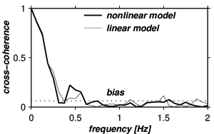
Figure 5: Cross-coherence between the measured and the simulated output, for a linear and a nonlinear model. Values close to or below the bias level are not considered to be significant [Bendat and Piersol, 1986].

As mentioned before, there are several reasons to believe that a low-order model should capture most of the dynamics, especially in weak turbulence. This can be verified in different ways. Ritz and Powers [1986] considered nonlinear correlations between linear and nonlinear terms. We focus instead on the predictive capacity of the models, using the cross-validation defined in (26). We built first-, second-, and third-order models, all of which were tested against the data (the third order model could could not have as much frequency resolution because of its large number of degrees of freedom).

Figure 5 shows the result of the cross-validation applied to a linear and to a quadratically nonlinear model. Both models succeed relatively well in predicting the low frequency part of the AMPTE-IRM waveform. The performance drop with increasing frequency is a well-known effect, which cannot be compensated simply by increasing the model complexity. Possible causes are the decreasing signal-to-noise ratio, the finite lifetime and the dispersion of the wave packets, fluctuations in the solar wind velocity, and the 1-D approximation of our model.

The central result here is the close performance of the linear and the quadratic models, which attests the predominantly linear behavior of the wave field and a priori supports the choice of a low-order model. A notable exception occurs around $f=\omega/2\pi\approx 0.5$ Hz, where a quadratic model brings some improvement. This shall see later that nonlinear effects are indeed important in that frequency band.

7.2 Choice of the Frequency Range

There is a strong impetus for reducing as much as possible the number of degrees of freedom of our model. One way of doing this is by reducing the frequency range. As shown in Figure 5, fluctuations with frequencies beyond 0.8 Hz cannot be satisfactorily modeled and so one may safely truncate the frequency range at 1 Hz, above which the power spectral content becomes negligible anyway. We checked that higher-order coherence functions vanish as well above 1 Hz.

A further reduction in the number of degrees of freedom can in principle be achieved by discarding in the linear system (equation (18)) those columns of the matrix which are not significantly correlated with the output ${\mathsf{Y}}_{\omega}$. Such a reduction is permitted when the nonlinear interactions are very localized in frequency space.

7.3 Choice of the Mesh Resolution

The frequency spacing $\delta\omega$ (which is proportional to $1/N_{\omega}$) must be small enough to distinguish important features such as spectral lines and yet as large as possible to prevent the model from being overdetermined. Since we deal with broadband turbulence, a relatively coarse mesh should a priori suffice. Nonlinear parametric models [Billings, 1980] may be needed when closely spaced lines must be resolved.

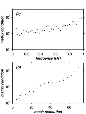
Figure 6: Condition number of the matrix ${\mathsf{U}}_{\omega}$ versus (a) frequency with a fixed mesh resolution $N_{\omega}=20$, and (b) versus $N_{\omega}$ for a fixed frequency $f\approx 0.5$ Hz.

The impact of the mesh resolution is best revealed by the condition number [Golub and Van Loan, 1993] of the matrix ${\mathsf{U}}_{\omega}$, which gives a figure of merit for the ill-posedness of (18). The condition number is at best $1$ and typically should not exceed a few hundreds; its value is displayed in Figure 6 for different mesh resolutions. The condition degrades for increasing $N_{\omega}$ because more coefficients have to be estimated from the same sample; another reason is the increasing collinearity between columns of ${\mathsf{U}}_{\omega}$. These problems may be partially alleviated by projecting ${\mathsf{U}}_{\omega}$ on an orthogonal basis [see Im et al., 1996].

From these considerations, we choose a quadratically nonlinear model with $N_{\omega}=40$ and a frequency range from 0 to 1 Hz.

8 Linear Properties of the Wave Field

We now focus on the interpretation of the model and start with the leading term, which is the linear one. The linear kernel $\Gamma_{\omega}$ can conveniently be split into a real and an imaginary part

$$\Gamma(\omega)=\overline{\gamma}(\omega)+j\overline{\theta}(\omega)\ .$$ (27)

The imaginary part

$$\overline{\theta}(\omega)\approx\frac{1}{\delta t}{\mathrm{I}m}\left[\log\langle U_{\omega}^{*}\>Y_{\omega}\rangle\right]$$ (28)

expresses the average phase-shift undergone by the wave-packets as they move from one spacecraft to the other. It is therefore related to the wavenumber $\overline{k}$, averaged over the power spectral density, by $\overline{k}=\overline{\theta}/v_{sw}$.

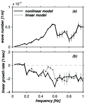
Figure 7: (a) Imaginary and (b) real parts of the linear transfer function, as calculated using a linear and a nonlinear model. Error bars correspond to $\pm$ one standard deviation. The results are inaccurate above 0.6 Hz because the model fails to reproduce small-amplitude fluctuations correctly.

The average dispersion relation $\overline{k}(\omega)$ is shown in Figure 7. Given our timing convention, we are in the plasma rest frame and positive wavenumbers correspond to a sunward motion. Error bars correspond to one standard deviation as calculated from the least-squares fit of the model.

Figure 7 shows that the wave field is essentially dispersionless up to about 0.5 Hz. Above this frequency, the dispersion becomes positive, and high-frequency waves move ahead of low-frequency ones. We refer to previous work [Dudok de Wit et al., 1995] for a discussion on this, but just note that the modeling fails above 0.6 Hz, presumably because of the low power spectral density.

The real part of the Volterra kernel

$$\overline{\gamma}(\omega)\approx\frac{1}{\delta t}\left(\frac{\left|\langle U_{\omega}^{*}\>Y_{\omega}\rangle\right|}{\langle U_{\omega}^{*}\>U_{\omega}\rangle}-1\right)\ ,$$ (29)

gives the linear growth averaged as before over $k$. The results are shown in Figure 7. The negative value of $\overline{\gamma}(\omega)$ attests a damping of the waves, so we conclude that the wave field is on average linearly stable. An exception occurs below 0.2 Hz, where the wave field grows as it goes from one spacecraft to the other. Although this growth rate is subject to a rather large uncertainty, its positive sign is statistically significant. Interestingly, this unstable frequency band coincides with that of the SLAMS and therefore lends strong support to the instability of these structures. The unstable nature of the SLAMS has already been conjectured [Schwartz and Burgess, 1991], but we now have the first direct evidence for a dynamic evolution.

From the linear growth rate, one can estimate the characteristic time needed for the SLAMS to grow, assuming that there is no nonlinear mechanism to saturate such a growth. We find $\tau=1/\overline{\gamma}\approx$ 10 s, a value that should be compared to the characteristic lifetime of these structures

$$\frac{\tau}{T}=\frac{\overline{\theta}}{\overline{\gamma}}=\frac{{\mathrm{I}m}(\Gamma)}{{\mathrm{R}e}(\Gamma)}\approx 10\%\ .$$ (30)

This ratio is sufficiently small to justify a linearization of the growth process (and the weak turbulence approximation) and yet large enough to make the instability of the SLAMS easily detectable.

It is instructive to check here the assumption of nonlinearity by comparing these results to what we would obtain by fitting a linear model. The two growth rates are compared in Figure 7 and a discrepancy appears. We attribute this to the energy redistribution process between Fourier modes, which is neglected in the linear model and correctly taken into account in the nonlinear one. As we shall see later, the linear model tries to compensate an energy flux around 0.5 Hz by artificially lowering the damping rate. The use of a nonlinear model for assessing linear properties should therefore not be underestimated.

9 Nonlinear Properties of the Wave Field

We now consider the properties of the second-order Volterra kernel. As mentioned before, this is the only nonlinear term we can reliably estimate given the amount of data.

9.1 Phase Couplings

The second-order Volterra kernels $\Gamma(\omega_{1},\omega_{2})$ as such are not very informative, even though they contain all the relevant information on the quadratic couplings. Better insight can be gained by looking at the the cross-bicoherence (equation (24)), which is indicative of the strength of the quadratic interactions. In the same way, we compute the cross-tricoherence (equation (25)) to study cubic interactions, even though the third-order kernel itself cannot be reliably estimated.

Figure 8: The cross-bicoherence, displayed in the principal domain, for frequency-adding interactions only ($f_{1},f_{2}\geq 0$). Its value is bounded between 0 and 1.

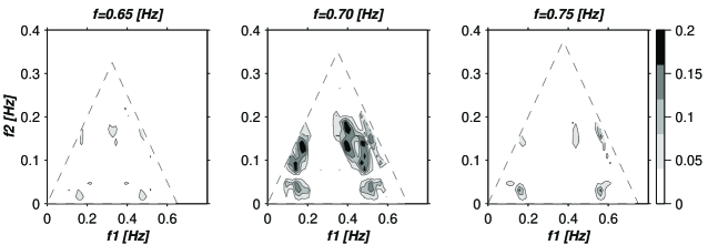
Figure 9: Cross-tricoherence, shown here for interactions of the type $f_{1}+f_{2}+f_{3}=f$ Hz only, with $f_{1},f_{2},f_{3}\geq 0$. Values are bounded between 0 and 1, and the dashed line refers to the principal domain.

The cross-bicoherence and cross-tricoherence are displayed in Figures 8 and 9 respectively. In both Figures 8 and 9 the support is restricted to the nonredundant and positive frequency domain. The most conspicuous result is the presence of local maxima that attest the existence of phase couplings between specific spectral modes. We conclude from the cross-bicoherence that a significant phase coupling occurs between wave packets whose frequencies satisfy the summation rule $0.1+0.45=0.55$ Hz. The cross-tricoherence reveals a significant coupling for $0.1+f_{l}+f_{m}=0.55$ Hz, with $0.1\leq f_{l}\leq f_{m}\leq 0.55$ Hz. Both couplings relate wave packets whose frequencies are about 0.1 Hz and 0.55 Hz, with possibly some intermediate frequencies to enable the phase coupling. As shown in previous work [Dudok de Wit and Krasnosel’skikh, 1995], these characteristic frequencies respectively correspond to the SLAMS and to the discrete whistler wave packets that frequently occur at the leading edge of SLAMS. The nonzero cross-bicoherence and cross-tricoherence thus reveal the existence of a causal relationship between the SLAMS and the whistlers.

9.2 Energy Transfers

The last step now consists in determining whether the SLAMS and the whistlers are exchanging energy or if they are just remnants of a process that took place farther upstream. To do so, we compute the quadratic energy transfer function, shown in Figure 10. A significant energy flux appears at $0.1+0.45\rightarrow 0.55$ Hz, which corresponds to an energy transfer going from the SLAMS to the whistlers. This is the central result of our paper, from which we conclude that the whistlers are much more likely to be a decay product of the SLAMS than some instability triggered by them. Such a conclusion was partly anticipated, but only the energy transfer function can give unambiguous evidence for it.

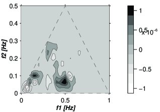
Figure 10: Spectral energy transfer rate (in arbitrary units) using the same representation as for the cross-bicoherence. The confidence interval is about equal to the spacing between two contour levels.

The other patterns in Figure 10 also have an interpretation. The $0.1+0.1\rightarrow 0.2$ Hz transfer corresponds a first harmonic generation due the nonlinear steepening of the SLAMS.

9.3 Power Balance

Further insight into the dynamics of the wave field can be gained by studying the power balance. Consider the truncated second-order wave kinetic equation (equation (3.4))

$$\frac{\partial{E_{\omega}}}{\partial t}\;=\;2\overline{\gamma}_{\omega}\,E_{\omega}+2\sum_{\stackrel{{\scriptstyle\omega_{1},\omega_{2}}}{{\omega=\omega_{1}+\omega_{2}}}}T_{\omega_{1},\omega_{2}}\ .$$ (31)

Stationarity ($\partial{E_{\omega}}/\partial{t}=0$) is approximately reached when the two terms on the right-hand side cancel; these two terms are plotted in Figure 11.

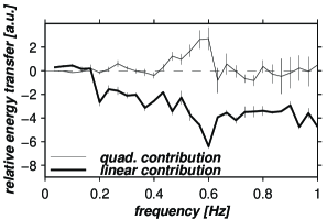
Figure 11: Relative change of spectral power showing the contributions of the linear growth term ($2\overline{\gamma}_{\omega}$), and of the three-wave interactions ($2\sum T_{\omega_{1},\omega_{2}}/E_{\omega}$). The results are unreliable above 0.6 Hz.

At low frequencies ($f<$ 0.2 Hz) the growth rate and the energy transfer indeed approximately cancel each other and so the wave field amplitude should not vary much in time. We conclude that the decay of the SLAMS is approximately compensated by their linear instability. At higher frequencies the power balance becomes increasingly negative, suggesting that the waves are on average damped. A plausible damping mechanism would be resonant particle damping, but the various approximations made in our model may actually cause the damping to be overestimated at high frequencies (see the appendix).

9.4 Interpretation

A coherent scenario now emerges, which is schematized in Figure 12. The SLAMS appear as dynamically evolving structures that progressively grow out of the wave field by drawing energy from energetic ions. As they grow, nonlinear effects enter into play. The transfer function analysis shows that the dominant process is a nonlinear wave interaction that compensates the growth by an energy transfer toward high-frequency whistler waves (some energy may also go into low-frequency waves). The whistler waves in turn move ahead of the SLAMS because of the positive dispersion and are eventually damped by dissipation.

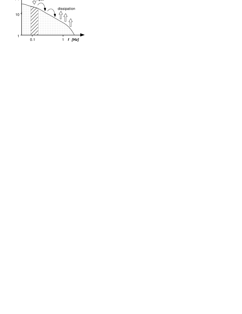
Figure 12: Schematic representation of the power spectral density of the magnetic field, showing where the energy enters the wave field and where it is transferred before being dissipated. The SLAMS are located in the hatched zone.

The emergence of such right-handed circularly polarized waves out of the left-handed linearly polarized SLAMS shows some striking similarities with the expected behavior of solitary waves [Hada et al., 1989] and also recalls the behavior of shock fronts in weakly dispersive media [Karpman, 1975]. All these phenomena have in common a competition between dispersion and nonlinearity, whose distinctive manifestation is the resilience of the shape of the SLAMS.

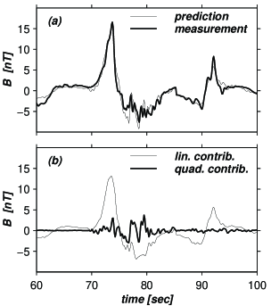
Figure 13: Excerpt of Figure 2, showing one component of the magnetic field with a typical SLAMS at $t=$70-76 s and its whistler precursor at $t=$76-82 s. (a) The wave field measured by AMPTE-IRM is compared with the model prediction. (b) The model prediction is split into its linear and quadratic constituents.

To finish, let us visualize how the nonlinear interactions show up in the time domain. Figure 13 represents a particular SLAMS with the measured and the predicted wave field. We decomposed the latter into its linear and quadratic contributions. As expected, the linear contribution captures most of the dynamics but does not correctly reproduce the fast oscillations at the leading edge of the SLAMS and which correspond to a distorted whistler wave packet. A quadratic contribution is definitely needed here to fit the observations.

10 Conclusions

This study reveals how Volterra models can be used to infer nonlinear properties from a turbulent wave field using two-point measurements. Provided the model is carefully validated, it can give direct access to the wave field growth rate and to the energy transfer function.

We used the Volterra approach to analyze plasma turbulence as observed just upstream the Earth’s quasi-parallel bow shock by the AMPTE spacecraft. An important feature of the wave field is the occurrence of nonlinear magnetic structures termed SLAMS. Our analysis attests the coexistence of two competing mechanisms: the SLAMS progressively grow by drawing energy from hot ions but before overturning they saturate and release the excess of energy into high frequency whistler waves that move ahead of them due to dispersion. The dynamical evolution of the SLAMS and their differential velocity [Schwartz et al., 1992] support the conjecture in which they supposedly merge into an extended front that constitutes the bow shock.

The method we advocate here is applicable to other types of events provided they are recorded by multiple-spacecraft missions whose configuration satisfies some constraints (see the appendix). A number of improvements can be made, such as the generalization to vector fields, which would allow anisotropy effects to be included. In some cases the addition of a source term that enforces the stationarity of the wave field may be desirable.

Acknowledgments

We would like to thank Steven Schwartz for making valuable comments on the manuscript. Discussions with Arnaud Masson on the tricoherence and with Mikhail Balikhin are also acknowledged.

Michel Blanc thanks Hans Pécseli and Vincenzo Carbone for their assistance in evaluating this paper.

Appendix A Appendix: Limitations of the Technique

The nonlinear transfer function cannot be meaningfully assessed without keeping in mind several limitations and potential pitfalls. The most important ones are listed here.

A.1 One-Dimensional Approach

Restricting the analysis to two probes means that we can only study structures propagating parallel to the spacecraft separation vector. Structures propagating obliquely to it will cause an overestimation of the damping rate and an underestimation of the energy transfer.

A.2 Anisotropy

Our scalar model can in principle be generalized to vectorial quantities with the interesting perspective of addressing anisotropy effects. The price to pay for this is a larger number of degrees of freedom. Neglecting the vectorial nature of the variables may actually alter the power balance because of the omission of the wave field rotation. Although the rotation we measure is quite small, we believe this effect to be sufficient to accentuate the globally negative trend observed in Figure 11.

A.3 Taylor Hypothesis

Another problem comes from the connection between frequency and wavenumber space, for which the Taylor hypothesis was invoked at the beginning. The dispersionless approximation remains valid up to about 0.5 Hz. Above this limit, the dispersion becomes positive and hence the resonance conditions (equations (3)-(5)) are altered. The finite frequency resolution of the wavelets can easily accommodate such small detunings in the resonance conditions.

A.4 Validity of the Model

The weakest point of our approach is the difficulty in justifying the validity of a low-order model in a definite way. A quadratically nonlinear model suffices for describing the main features of the wave field (section 7), but Figure 9 reminds us that cubic interactions cannot be neglected. Although we are confident in the conclusions drawn from our second-order model, one should keep in mind that the results remain approximate as long as cubic and possibly even higher-order effects are not taken into account.

A.5 Calibration of the Probes

It is essential that the two probes (the magnetometers here) be properly calibrated and have the same instrumental transfer function for our analysis to be meaningful. Although this is not a problem for the frequency range we are considering, it may exclude diagnostics that have either an unreliable calibration or a nonlinear response.

References

• Bale, S. D., D. Burgess, P. J. Kellogg, K. Goetz, R. L. Howard, and S. J. Monson, Evidence of three-wave interactions in the upstream solar wind, Geophys. Res. Lett., 23, 109–112, 1996.

• Balk, A. M., V. E. Zakharov, and S. V. Nazarenko, Nonlocal turbulence of drift waves, Sov. Phys. JETP, 71, 249–260, 1990.

• Bendat, J. S., Nonlinear System Analysis and Identification from Random Data, John Wiley, New York, 1990.

• Bendat, J. S. and A. G. Piersol, Random Data: Analysis and Measurement Procedures, 2nd ed., John Wiley, New York, 1986.

• Billings, S. A., Identification of Nonlinear Systems-A Survey, IEE Proc., Part D, 127, 272–285, 1980.

• Brillinger, D. R., The identification of polynomial systems by means of higher order spectra, J. Sound Vibr., 12, 301–313, 1970.

• Dudok de Wit, T., and V. V. Krasnosel’skikh, Wavelet bicoherence analysis of strong plasma turbulence at the Earth’s quasiparallel bow shock, Phys. Plasmas, 2, 4307–4311, 1995.

• Dudok de Wit, T., V. V. Krasnosel’skikh, S. D. Bale, M. Dunlop, H. Lühr, S. J. Schwarz, and L. J. C. Woolliscroft, Determination of dispersion relations in quasi-stationary plasma turbulence using dual satellite data, Geophys. Res. Lett., 22, 2653–2656, 1995.

• Farge, M., N. Kevlahan, V. Perrier, and E. Goirand, Wavelets and turbulence, Proc. IEEE, 84, 639–669, 1996.

• Golub, G. H., and C. F. Van Loan, Matrix Computations, 2nd ed., Johns Hopkins Press, Baltimore, Md., 1989.

• Hada, T., C. F. Kennel, and B. Buti, Stationary nonlinear Alfvén waves and solitons, J. Geoph. Res., 94, 65–77, 1989.

• Horton, W. and A. Hasegawa, Quasi-two-dimensional dynamics of plasmas and fluids Chaos, 4, 227–251, 1994.

• Im, S., E. J. Powers, and I. S. Park, Applications of higher-order statistical signal processing to nonlinear phenomena, in Transport, Chaos and Plasma Physics II, edited by S. Benkadda, F. Doveil, and Y. Elskens, pp. 74–88, World Sci., Singapore, 1996.

• Kadomtsev, B. B., Plasma Turbulence, Pergamon, New York, 1982.

• Karpman, V. I., Non-linear Waves in Dispersive Media, Pergamon, New York, 1975.

• Kim, J. S., R. D. Durst, R. J. Fonck, E. Fernandez, A. Ware, and P. W. Terry, Technique for the experimental estimation of nonlinear energy transfer in fully developed turbulence, Phys. Plasmas, 3, 3998–4009, 1996.

• Kim, K. I., and E. J. Powers, A digital method of modeling quadratically nonlinear systems with a general random input, IEEE Trans. Acoust. Speech Signal Process., ASSP-36, 1758–1769, 1988.

• Kim, Y. C., and E. J. Powers, Digital bispectral analysis and its applications to nonlinear wave analysis, IEEE Trans. Plasma Sci., PS-7, 120–131, 1979.

• Krasnosel’skikh, V. V., and F. Lefeuvre, Strong Langmuir turbulence in space plasmas, the problem of recognition, in START: Spatio-temporal analysis for resolving plasma turbulence, Doc. WPP-047, pp. 237–242, Eur. Space Agency, Paris, 1993.

• Kravtchenko-Berejnoi, V., F. Lefeuvre, V. V. Krasnosel’skikh, and D. Lagoutte, On the use of tricoherent analysis to detect non-linear wave-wave interactions, Signal Proc., 42, 291–309, 1995.

• Krommes, J. A., Systematic statistical theories of plasma turbulence and intermittency: Current status and future prospects, Phys. Rep., 283, 5–48, 1997.

• LaBelle, J., and E. J. Lund, Bispectral analysis of equatorial spread $F$ density irregularities, J. Geoph. Res., 97, 8643–8651, 1992.

• Lagoutte, D., F. Lefeuvre, and J. Hanasz, Application of bicoherence analysis in study of wave interactions in space plasma, J. Geoph. Res., 94, 435–442, 1989.

• Lii, K. S., K. N. Helland, and M. Rosenblatt, Estimating three-dimensional energy transfer in isotropic turbulence, J. Time Ser. Anal., 3, 1–28, 1982.

• Ljung, L., System Identification, Prentice-Hall, Englewood Cliffs, N. J., 1987.

• Mann, G., H. Lühr, and W. Baumjohann, Statistical analysis of short large-amplitude magnetic field structures in the vicinity of the quasi-parallel bow shock, J. Geoph. Res., 99, 13315–13323, 1994.

• Mendel, J. M., Tutorial on higher-order statistics (spectra) in signal processing and system theory: Theoretical results and some applications, Proc. IEEE, 79, 278–305, 1991.

• Monin, A. S., and A. M. Yaglom, Statistical Fluid Mechanics, vol. 2, MIT Press, Cambridge, Mass., 1975.

• Musher, S. L., A. M. Rubenchik, and V. E. Zakharov, Weak Langmuir turbulence, Phys. Rep., 252, 177–274, 1995.

• Nam, S. W., and E. J. Powers, Application of higher order spectral analysis to cubically nonlinear system identification, IEEE Trans. Acoust. Speech Signal Process., ASSP-42, 1746–1765, 1994.

• Omidi, N., and D. Winske, Steepening of kinetic magnetosonic waves into shocklets: simulations and consequences for planetary shocks and comets, J. Geoph. Res., 95, 2281–2300, 1990.

• Pécseli, H. L., and J. Trulsen, On the interpretation of experimental methods for investigating nonlinear wave phenomena, Plasma Phys. Controlled Fusion, 25, 1701–1715, 1993.

• Pécseli, H. L., J. Trulsen, A. Bahnsen, and F. Primdahl, Propagation and nonlinear interaction of low-frequency electrostatic waves in the polar cap $E$ region, J. Geoph. Res., 98, 1603–1612, 1993.

• Priestley, M. B., Spectral Analysis and Time Series, Academic Press, San Diego, Calif., 1981.

• Ritz, C. P., and E. J. Powers, Estimation of nonlinear transfer functions for fully developed turbulence, Phys. D, 20, 320–334, 1986.

• Ritz, C. P., E. J. Powers, R. W. Miksad, and R. S. Solis, Nonlinear spectral dynamics of a transitioning flow, Phys. Fluids, 31, 3577–3588, 1988a.

• Ritz, C. P., et al., Advanced plasma fluctuation analysis techniques and their impact on fusion research, Rev. Sci. Instrum., 59, 1739–1744, 1988b.

• Ritz, Ch. P., E. J. Powers, and R. D. Bengtson, Experimental measurement of three-wave coupling and energy cascading, Phys. Fluids B, 1, 153–163, 1989.

• Schetzen, M., The Volterra and Wiener Theories of Nonlinear Systems, John Wiley, New York, 1980.

• Scholer, M., Upstream waves, shocklets, short large-amplitude magnetic structures and the cyclic behavior of oblique quasi-parallel collisionless shocks, J. Geoph. Res., 98, 45–57, 1993.

• Schwartz, S. J., and D. Burgess, Quasi-parallel shocks: A patchwork of three-dimensional structures, Geophys. Res. Lett., 18, 373–376, 1991.

• Schwartz, S. J., D. Burgess, W. P. Wilkinson, R. L. Kessel, M. Dunlop, and H. Lühr, Observations of short large-amplitude magnetic structures at a quasi-parallel shock, J. Geoph. Res., 97, 4209–4227, 1992.

• Thomsen, M. F., D. T. Gosling, S. J. Bame, and C. T. Russell, Magnetic pulsations at a quasi-parallel shock, J. Geoph. Res., 95, 957–966, 1990.

• Tick, L. J., The estimation of “transfer functions” of quadratic systems, Technometrics, 3, 563–567, 1961.

• Uberoi, M. S., Energy transfer in isotropic turbulence, Phys. Fluids, 6, 1048–1056, 1963.

• van Milligen, B. P., E. Sánchez, T. Estrada, C. Hidalgo, B. Brañas, B. Carreras, and L. García, Wavelet bicoherence: a new turbulence analysis tool, Phys. Plasmas, 2, 3017–3032, 1995.

• Van Atta, C. W., and W. Y. Chen, Measurements of spectral energy transfer in grid turbulence, J. Fluid Mech., 38, 743–763, 1969.

• Wiener, N., Nonlinear Problems in Random Theory, MIT Press, Cambridge, Mass., 1958.

• Winske, D., N. Omidi, K. B. Quest, and V. Thomas, Reforming supercritical quasi-parallel shocks, 2, mechanism for wave generation and front reformation, J. Geoph. Res., 95, 18821–18827, 1990.

• Zakharov, V. E., S. L. Musher, and A. M. Rubenchik, Hamiltonian approach to the description of non-linear plasma phenomena, Phys. Rep., 129, 285–366, 1985.