A Bayesian test for the appropriateness of a model in the biomagnetic inverse problem

Abstract

This paper extends the work of Clarke [e:Clarke94] on the Bayesian foundations of the biomagnetic inverse problem. It derives expressions for the expectation and variance of the a posteriori source current probability distribution given a prior source current probability distribution, a source space weight function and a data set. The calculation of the variance enables the construction of a Bayesian test for the appropriateness of any source model that is chosen as the a priori infomation. The test is illustrated using both simulated (multi-dipole) data and the results of a study of early latency processing of images of human faces.

Keywords

Biomagnetic inverse problem, Bayesian.

1 Introduction

The magnetoencephalographic (MEG) inverse problem (sometimes known as the biomagnetic inverse problem) is the process of identifying the source current distribution inside the brain that gives rise to a given set of magnetic field measurements outside the head. The problem is difficult because the detectors are limited in number and are sensitive to widespread source currents, and because of the existence of silent and near-silent sources. ’Silent sources’ are configurations of current density inside the brain which give zero magnetic field outside the head (e.g. all radial sources are silent when the head is modelled as a conducting sphere). It follows that the general biomagnetic inverse problem is ill-posed and under-determined.

The most common way of reducing the problem and rendering it tractable is by characterising the source in terms of a limited number of effective current dipoles. Such source descriptions provide links with the dominant functional architecture model of the brain in which processing is described in terms of localised activity with interactions between essentially separate regions. Multiple dipole models have enjoyed considerable success in the analysis of sensory and motor cortex (e.g. [e:Vanni96, e:Buchner95, e:Mauguiere97, e:Hoshiyama97]).

Growing evidence for the existence of more diffuse brain networks have led to an interest in distributed source algorithms. Several have been proposed [Hamalainen84, e:Hamalainen94, p:Ioannides89, e:Wang92, e:Marqui94, e:Gorodnitsky95]. These algorithms have been designed to cope with the non-uniqueness of the problem, primarily by restriction of the source space and by regularisation. Each algorithm leads to a unique solution (from the infinite number available) through its particular choice of source basis, weight functions, noise assumptions, and, in many cases, cost function. There has been an extended debate about the accuracy and value of these methods. This proceeds at two levels; the technical ability of the various algorithms to recover a simulated source distribution (often quoted in terms of one or more source current dipoles), and the electrophysiological appropriateness of the type of source structure favoured by particular algorithm parameters. So, for example the simple minimum norm solution [e:Hamalainen94], which tends to produce a grossly smeared and superficial source distribution may be compared with the LORETA solution [e:Marqui94] which favours smooth but regionally confined current distributions. The issues have been fully debated in recent conferences [e:ISBET-loreta, e:Wood98]).

The many to one nature of the mapping of sources to magnetic fields suggests that a probabilistic approach to reconstructing the sources from the magnetic field could be used. A Bayesian probabilistic approach was first proposed by Clarke [e:Clarke94]. More recently, Baillet et al have described an iterative approach which combines both spatial and temporal constraints within a unified Bayesian framework designed to allow the estimation of source activity that varies rapidly with position, e.g. across a sulcus [e:Baillet97]. Schmidt et al have developed a probabilistic algorithm in which a bridge is made between distributed and local source solutions through the use of a regional descriptor within the source representation [e:Schmidt97]. In this case, a Monte Carlo method is used in the absence of an analytic solution for the expectation value of the source current.

Here, we are proposing an alternative Bayesian approach. It includes the explicit assumption of both a prior source current probability distribution and a source space weight function, and allows the calculation of the expectation and variance of the a-posteriori source current probability distribution. The derivation of these quantities is detailed in Section 3. The inclusion of the prior probability and the calculation of the variance provide a means by which the consistency of a model (assumed as the prior) can be tested against the data to reveal those parts of the source distribution that are statistically robust and, conversely, where the model is inadequate. Numerical calculation of significance is possible. A straightforward extension of this idea is the direct comparison of two data sets to reveal where, within a given model, there are significant differences in their associated source distributions. In the final part of this paper, both simulated and real data will be used to illustrate these various uses of the technique.

2 Specification of the problem

The arrangement of sources and detectors for the biomagnetic inverse problem is shown in Figure 1. The sources giving rise to the measurements are assumed to be restricted within a source space $Q$, which may be smaller than the whole head volume (e.g. if the sources are assumed to be cortical). The current density within the volume $Q$ is assumed to belong to the space of square integrable vector fields on $Q$, which we call $J$.

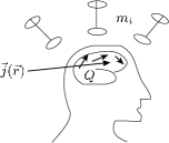
Figure 1: A schematic experimental geometry.

The measurement process typically gives successive sets of data ($\sim 100$ channels) every millisecond. In this paper the data for each time instant is processed independently, and the data from a single time instant is collected into a vector $\mbox{$\tilde{m}$}\in\mbox{$\mathbb{R}$}^{N}$. If $\mbox{$\vec{j}$($\vec{r}$)}\in J$ then the measurement process can be represented by a functional $z:J\rightarrow\mbox{$\mathbb{R}$}^{N}$. A subscript notation will be used to identify the sensor, i.e. $z_{i}$ is the ideal reading from the $i$th sensor. So the basic equation is:

$$\mbox{$\tilde{m}$}_{i}=z_{i}(\mbox{$\vec{j}$})+e_{i}$$

where the $e_{i}$ are the measurement errors, which are assumed to be normally distributed with zero mean and covariance matrix $\alpha^{2}D$ (where $\alpha$ is the standard deviation of the errors and $D$ is a symmetric, positive definite matrix).

To compute the functional $z(\ )$ on a computer (i.e. to solve the forward problem) requires a volume conductor model of the head. In this paper the precise model used is irrelevant, so the final results will be written in terms of $z$. This is done is via the Green’s functions $\vec{L}_{i}$ for the problem, which are defined by

$$z_{i}(\mbox{$\vec{j}$})=\int_{Q}\mbox{$\vec{L}_{i}$}\mbox{($\vec{r}$)}\cdot\mbox{$\vec{j}$($\vec{r}$)}\;{\rm d}\vec{r}$$

Stated simply, the inverse problem is to estimate $\vec{j}$($\vec{r}$) given the data vector $\tilde{m}$. Obviously the given data are not enough to determine $\vec{j}$($\vec{r}$) uniquely (for several reasons). The approach adopted here starts from the same point as used in Clarke [e:Clarke94], a statement of Bayes’s theorem:

$$\mbox{$\cal P$}(\mbox{$\vec{j}$}\in A|m\in B)=\frac{\mbox{$\cal P$}(m\in B|\mbox{$\vec{j}$}\in A)\mbox{$\cal P$}(\mbox{$\vec{j}$}\in A)}{\mbox{$\cal P$}(m\in B)}$$

where $A$ is a set of currents and $B$ is a set of measurements. This equation reads, the a posteriori probability of a current set $A$ after the measurement $B$ is proportional to the probability of producing the measurement $B$ given that the current is in the set $A$ times the a priori probability of the current set $A$. ($\mbox{$\cal P$}(m\in B)$ is a constant for any measurement set $B$).

In this paper the probability distributions (both the prior probability and the errors) are assumed to be gaussian and so it is permissible to work with probability density functions. A further simplification is achieved by shrinking the measurement set $B$ to a single point $\{\mbox{$\tilde{m}$}\}$ (this ignores the finiteness of the precision of the measurements). Equation 2 then becomes:

$$\rho_{\mbox{$\tilde{m}$}}(\mbox{$\vec{j}$})\propto\rho(\mbox{$\vec{j}$})\;\times\;\epsilon(\mbox{$\tilde{m}$}-z(\mbox{$\vec{j}$}))$$

where $\rho$ is the a priori distribution, $\rho_{\mbox{$\tilde{m}$}}$ is the a posteriori distribution and $\epsilon$ is the error distribution. Throughout the paper, probability density functions will only be determined up to a constant. The constant of proportionality is found by requiring that the probability is normalised to one. In this paper both $\rho$ and $\epsilon$ are assumed to be Gaussian and then $\rho_{\mbox{$\tilde{m}$}}$ is calculated to be Gaussian. An error probability density function $\epsilon$ consistent with the Gaussian assumption may be written:

$$\epsilon(e)\propto\exp\left\{-\frac{1}{2\alpha^{2}}{e}^{\mbox{\rm\tiny T}}{D}^{-1}e\right\}$$

This generally valid expression will be retained throughout the derivation in this paper. In practice, the noise covariance matrix $D$ may be difficult to estimate and, for simplicity, the simple form $D=I$ will be used in the later illustrations.

3 Derivation

In this section formulae for the maximum likelihood current distribution and also the expected error distribution are derived under specific assumptions. First, an inner product on $J$ is defined by:

$$\left\langle\mbox{$\vec{j}$}_{1}\;,\;\mbox{$\vec{j}$}_{2}\right\rangle=\int_{Q}\frac{\mbox{$\vec{j}$}_{1}\mbox{($\vec{r}$)}\cdot\mbox{$\vec{j}$}_{2}\mbox{($\vec{r}$)}}{\omega\mbox{($\vec{r}$)}}\;{\rm d}\vec{r}$$

where $\omega\mbox{($\vec{r}$)}$ is a weighting distribution defined on the source space $Q$. This provides a method of inputting prior information of the location of sources (e.g. gained from MRI images) into the algorithm.

Clarke [e:Clarke94] assumed that the maximum likelihood prior current density was identically zero. Here that restriction is avoided and an arbitrary prior current ${\vec{j}}^{p}$ will be introduced as a parameter of the method. The a priori probability distribution on $J$ is defined using ${\vec{j}}^{p}$ and the inner product:

$$\rho(\mbox{$\vec{j}$})\propto\exp\left\{-\frac{1}{2\beta^{2}}\left\langle\mbox{$\vec{j}$}-\mbox{${\vec{j}}^{p}$}\;,\;\mbox{$\vec{j}$}-\mbox{${\vec{j}}^{p}$}\right\rangle\right\}$$

where $\beta$ is the assumed a priori standard deviation.

To proceed further a basis is needed for $J$. A ‘natural’ choice is a basis that is related to the measurement functional $z$. So an obvious candidate is a basis derived from the adjoint map to the measurement map from $J$ to $\mbox{$\mathbb{R}$}^{N}$. This gives a map $\vec{z}:\mbox{$\mathbb{R}$}^{N}\rightarrow J$ (since $J$ is self-dual) defined by:

$$\left\langle\vec{z}(a)\;,\;\mbox{$\vec{j}$}\right\rangle={a}^{\mbox{\rm\tiny T}}z(\mbox{$\vec{j}$})$$

Explicitly this gives the set of linearly independent distributions $\{\omega\mbox{($\vec{r}$)}\mbox{$\vec{L}_{i}$}\mbox{($\vec{r}$)}\}$. This set is extended into a basis of $J$ that includes the silent sources by adding vectors $\{\mbox{$\vec{\cal L}_{i}$}\}$ which are chosen to be orthogonal to the $\{\omega\mbox{$\vec{L}_{i}$}\}$ i.e.

$$\left\langle\omega\mbox{$\vec{L}_{i}$}\;,\;\mbox{$\vec{\cal L}_{j}$}\right\rangle=0\hskip 28.45274pt\forall i,j$$

Since $\{\omega\mbox{($\vec{r}$)}\mbox{$\vec{L}_{i}$}\}\bigcup\{\mbox{$\vec{\cal L}_{i}$}\}$ is a basis of $J$ a general current density $\vec{j}$($\vec{r}$) can be written in terms of this basis as

$$\mbox{$\vec{j}$($\vec{r}$)}=\sum_{i=1}^{N}a_{i}\omega\mbox{($\vec{r}$)}\mbox{$\vec{L}_{i}$}\mbox{($\vec{r}$)}+\sum_{i}b_{i}\mbox{$\vec{\cal L}_{i}$}\mbox{($\vec{r}$)}$$

To simplify the notation the components of currents are written in column vector notation:

$$\mbox{$\vec{j}$}=\left(\begin{array}[]{@{}l@{}}a\\ b\end{array}\right),\qquad\mbox{${\vec{j}}^{p}$}=\left(\begin{array}[]{@{}l@{}}{a}^{p}\\ {b}^{p}\end{array}\right)$$

A simple computation gives

$$\left\langle\mbox{$\vec{j}$}-\mbox{${\vec{j}}^{p}$}\;,\;\mbox{$\vec{j}$}-\mbox{${\vec{j}}^{p}$}\right\rangle={\left(\begin{array}[]{@{}l@{}}a-{a}^{p}\\ b-{b}^{p}\end{array}\right)}^{\mbox{\rm\tiny T}}\left(\begin{array}[]{@{}ll@{}}P&0\\ 0&Q\end{array}\right)\left(\begin{array}[]{@{}l@{}}a-{a}^{p}\\ b-{b}^{p}\end{array}\right)$$

where $P_{ij}=\left\langle\omega\mbox{$\vec{L}_{i}$}\;,\;\omega\mbox{$\vec{L}_{j}$}\right\rangle$ and $Q_{ij}=\left\langle\mbox{$\vec{\cal L}_{i}$}\;,\;\mbox{$\vec{\cal L}_{j}$}\right\rangle$ since by construction $\left\langle\omega\mbox{$\vec{L}_{i}$}\;,\;\mbox{$\vec{\cal L}_{j}$}\right\rangle=0$.

Now the two a priori probability density functions (Equation 3 and Equation 2) may be combined with Bayes’s theorem (Equation 2) to obtain the a posteriori probability density:

$$\rho_{\mbox{$\tilde{m}$}}(\mbox{$\vec{j}$})\propto\exp\left\{-\frac{1}{2\beta^{2}}{\left(\begin{array}[]{@{}l@{}}a-{a}^{p}\\ b-{b}^{p}\end{array}\right)}^{\mbox{\rm\tiny T}}\left(\begin{array}[]{@{}ll@{}}P&0\\ 0&Q\end{array}\right)\left(\begin{array}[]{@{}l@{}}a-{a}^{p}\\ b-{b}^{p}\end{array}\right)\right\}\exp\left\{-\frac{1}{2\alpha^{2}}{(\mbox{$\tilde{m}$}-z(\mbox{$\vec{j}$}))}^{\mbox{\rm\tiny T}}{D}^{-1}(\mbox{$\tilde{m}$}-z(\mbox{$\vec{j}$}))\right\}$$

The task now is to manipulate this equation so that it is explicitly in the form of a gaussian distribution. As a first step the exponentials are combined:

$$\rho_{\mbox{$\tilde{m}$}}(\mbox{$\vec{j}$})\propto\exp\left\{-\frac{1}{2\alpha^{2}}\left[{\left(\begin{array}[]{@{}l@{}}a-{a}^{p}\\ b-{b}^{p}\end{array}\right)}^{\mbox{\rm\tiny T}}\left(\begin{array}[]{@{}ll@{}}\zeta P&0\\ 0&\zeta Q\end{array}\right)\left(\begin{array}[]{@{}l@{}}a-{a}^{p}\\ b-{b}^{p}\end{array}\right)+{(\mbox{$\tilde{m}$}-Pa)}^{\mbox{\rm\tiny T}}{D}^{-1}(\mbox{$\tilde{m}$}-Pa)\right]\right\}$$

where $\zeta=\alpha^{2}/\beta^{2}$ and $z(\mbox{$\vec{j}$})$ has been replaced by $Pa$. Next, the terms involving operators on $a$ are simplified by completing the square All constant terms can be absorbed into the normalization constant of the probability density function and are ignored in this derivation.

$$\halign to=0.0pt{\hskip\@centering$ \displaystyle# {} \@lign$\relax& \global\@eqcnt\@ne$ \displaystyle\@emptyord# \@lign$\hskip\@centering \relax& \global\@eqcnt\tw@\hskip\@centering#\relax\cr 0.0pt plus 1000.0pt$ \displaystyle\mbox{Operators on $a$} &{}= {(a-{a}^{p})}^{\mbox{\rm\tiny T}}\zeta P(a-{a}^{p})+{(\mbox{$\tilde{m}$}-Pa)}^{\mbox{\rm\tiny T}} {D}^{-1} (\mbox{$\tilde{m}$}-Pa) \\ $\hskip 0.0pt plus 1000.0pt&0.0pt plus 1000.0pt={a}^{\mbox{\rm\tiny T}}\zeta Pa-2{a}^{\mbox{\rm\tiny T}}\zeta P{a}^{p}+{a}^{\mbox{\rm\tiny T}}P{D}^{-1}Pa-2{a}^{\mbox{\rm\tiny T}}P{D}^{-1}\mbox{$\tilde{m}$}+\mbox{const.}\\&={a}^{\mbox{\rm\tiny T}}\left(\zeta P+P{D}^{-1}P\right)a-2{a}^{\mbox{\rm\tiny T}}[P{D}^{-1}\mbox{$\tilde{m}$}+\zeta P{a}^{p}]+\mbox{const.}\\&}$$