Front dynamics during diffusion-limited corrosion
of ramified electrodeposits.

Abstract

Experiments on the diffusion-limited corrosion of porous copper clusters in thin gap cells containing cupric chloride are reported. By carefully comparing corrosion front velocities and concentration profiles obtained by phase-shift interferometry with theoretical predictions, it is demonstrated that this process is well-described by a one-dimensional mean-field model for the generic reaction $\mbox{A}+\mbox{B\ (static)}\rightarrow\mbox{C\ (inert)}$ with only diffusing reactant (cupric chloride) and one static reactant (copper) reacting to produce an inert product (cuprous chloride). The interpretation of the experiments is aided by a mathematical analysis of the model equations which allows the reaction-order and the transference number of the diffusing species to be inferred. Physical arguments are given to explain the surprising relevance of the one-dimensional mean-field model in spite of the complex (fractal) structure of the copper clusters.

I Introduction

Diffusion-limited processes are ubiquitous in physics [1], chemistry [2] and biology [3]. Reaction-diffusion processes have been the subject of intense and continuous interest since the work of Smoluchowski [4, 5, 6]. A crucial feature of many such processes controlling pattern formation and reaction efficiency is the “reaction front”, a dynamic but localized region where reactions are most actively occurring which separates regions rich in the individual reactants. The simplest theoretical model of a reaction front, introduced more than a decade ago by Gálfi and Rácz [7], is the “mean-field” model for two initially separated species A and B reacting to produce an inert species C. Since then, the case of two diffusing reactants A and B has been thoroughly studied analytically [7, 8, 9, 10] and numerically [11, 12, 13, 14, 15, 16, 17, 18, 19, 20, 21], and some predictions of the mean-field model have been checked in experiments [21, 22, 23, 24, 25, 26, 27, 28, 29, 30].

In contrast, the case of only one diffusing reactant A and one static reactant B (confined on a fixed matrix) has not yet been studied experimentally. We show in this paper that the corrosion of a porous solid (B) immersed in a chemically active fluid suspension (A) can also be described by such a mean-field model. Some analytical [10, 31] and numerical [11, 32] studies exist for this case as well, but since it is more microscopically complex (for a real porous interface) than the case of two diffusing reactants (in a homogeneous medium) an experimental test of the model is needed.

The mean-field model of a planar reaction front for the chemical reaction

$$\mbox{A (diffusing) \ + \ B (static) \ $\rightarrow$ \ C (inert)},$$ (1)

postulates that the concentrations $\rho_{A}(X,T)$ and $\rho_{B}(X,T)$ of species A and B, respectively, evolve according to a pair of coupled partial differential equations [10, 31],

$$\frac{\partial\rho_{A}}{\partial T} = D_{A}\frac{\partial^{2}\rho_{A}}{\partial X^{2}}-R(\rho_{A},\rho_{B})$$ (2)

$$\frac{\partial\rho_{B}}{\partial T} = -R(\rho_{A},\rho_{B}),$$ (3)

where $D_{A}$ is the diffusion constant for species A and $R(\rho_{A},\rho_{B})$ is the reaction rate density. The most frequently used initial conditions assume that the reactants are uniformly distributed and completely separated at first, $\rho_{A}(X,0)=\rho_{A}^{o}H(X)$ and $\rho_{B}^{o}(X,0)=\rho_{B}^{o}H(-X)$, where $H(X)$ is the Heaviside unit step function. Such initial conditions are easier to reproduce in experiments than those involving uniformly mixed reactants. There are several assumptions behind Eqs. (2)–(3): $(i)$ The product $C$ is generated in small enough quantities that its presence does not significantly affect the dynamics; $(ii)$ The concentrations are dilute enough that the diffusivities are constant; $(iii)$ The fixed matrix containing reactant B (static) is porous enough that reactant A can freely diffuse through it; and $(iv)$ The reaction rate is a function of only the local concentrations and not any fluctuations or many-body effects (which is the “mean-field approximation”). It is common to make the mean-field approximation under the assumption $R(\rho_{A},\rho_{B})=k\rho_{A}^{m}\rho_{B}^{n}$, but in the interpretation of our experiments we will not assume anything about the form of $R(\rho_{A},\rho_{B})$ a priori since the reaction takes place at a solid-liquid interface. Moreover, this interface is highly ramified, and therefore, the underlying microscopic dynamics is expected to be more complex than for simple homogeneous kinetics.

In this paper we carefully test the validity of these assumptions with experiments on a particular porous-solid corrosion system: copper clusters corroded by a cupric chloride (CuCl₂) electrolyte. The clusters are obtained by a thin-gap cell electrodeposition from a CuCl₂ electrolyte at fixed current. This process builds a depletion layer of CuCl₂ ahead of the copper deposit. When the current is switched off, this CuCl₂ depletion layer relaxes toward the copper cluster bringing Cu²⁺ cations which react with copper according to:

CuCl₂ (aq)  +  Cu (solid, red)  $$\rightarrow$$  2 CuCl (solid, white) (4)

where the cuprous chloride (CuCl) is produced in the form of small (white) crystallites which drop down to the bottom of the cell.

In section II we describe the experimental set-up and the method used to prepare the porous clusters to be corroded. In section III we report the experimental evidence that our corrosion system behaves like a 1D diffusion-reaction process with one static reactant. In section IV, a mathematical analysis is presented which makes quantitative predictions based on the experimental data of section II, within the theoretical framework of the mean-field model, Eqs. (2)–(3). In the last section IV, the experimental results are revisited to refine the comparison with the theoretical model and to discuss in some detail of its physical limitations.

II Experimental Methods

A Apparatus

The experiments are performed in a thin-gap electrodeposition cell, which is depicted schematically in Fig. 1. The cell consists of an unsupported, aqueous solution of CuCl₂ confined to a narrow region of dimensions $W=5\mbox{cm}\times L=8\mbox{cm}\times\delta=50\mu\mbox{m}$ between two closely spaced, optically flat glass plates ($\lambda/4$ over 80mm$\times$50mm). Two parallel, ultrapure copper and silver wires (50$\mu$m diameter, Goodfellow 99% purity) are inserted between the two glass plates to act both as spacers and as electrodes. During the electrodeposition (prior to corrosion) the wires are polarized so that the silver wire acts as the cathode and the copper wire as the anode. The solutions of CuCl₂ (ACS reagent) are prepared from deionized water, carefully cleaned of any trace of dissolved oxygen by bubbling nitrogen through it for one hour. The anodic part of the cell (not shown in Fig. 1) is filled by a dilute solution of CuCl₂ to postpone the precipitation of the salt due to saturation effects by dissolution of the anode. The copper electrodeposits are all grown at constant current, and the entire experiment is performed at room temperature ($\approx 20^{\circ}C$).

Digitized color pictures of the copper clusters are obtained by direct imaging of the cluster through a lens, using a three-CDD camera coupled with an $8$-bit frame grabber from Data Translation driven by the public domain software IMAGE [33] which successively captures three RGB frames and from them reconstructs the color image.

A phase-shift Mach Zehnder interferometer is used independently to resolve the concentration field, averaged over the depth of the cell. A sketch of the interferometer can be found in ref.[34]. The interference patterns are recorded through a CCD camera coupled to the same frame grabber [33] with a 768$\times$512 pixel resolution. Phase-shift interferometry offers several significant advantages over traditional interferometry in that it provides an accurate reconstruction of the entire concentration field, using a set of successive interference pictures recorded for shifted values of the phase difference between two optical wavefronts, and can also be used as an holographic interferometer [35].

B Preparation of Copper Clusters by Electrodeposition

When current flows from the anode to the cathode, charge transfer occurs at the cathode, leading to the reduction of copper cations into copper metal according to [34, 36, 37]:

$\displaystyle\mbox{Cu}^{2+}+2\mbox{e}^{-}\rightarrow\mbox{Cu}\;\;.$

The actual mechanism of deposition is much more complex than this two electron transfer process since competitive reactions involving the solvent species are likely to occur. Nevertheless, in CuCl₂ electrolytes, we have observed that the formation of cuprous oxide (Cu₂O) in competition with copper by reduction of Cu²⁺ cations is not favored, contrary to what is observed in copper sulphate (CuSO₄) solutions [38, 39, 40], which can be partly explained by the strong adsorption and complexation properties of chloride anions [37]. This reduction process on the cathode implies a local depletion of the copper cations close to the cathode and, therefore, also their replenishment by a global transport process, namely diffusion. Although electromigration also contributes to transport, it does not act independently of diffusion in regions where electroneutrality is maintained [41], which means everywhere in the cell outside the $10-100\AA$ thick double layer [42, 43]. This often misunderstood fact was given a firm theoretical basis by Newman over 30 years ago in his asymptotic analysis of the transport equations for a rotating disk electrode [44], but only recently has it been quantitatively verified in experiments (by our group) for the case of constant boundary flux at a fixed cathode [34, 36]. In summary, the theoretical and experimental evidences indicate that in the absence of convection the concentration $\rho_{A}$ of a dilute, binary electrolyte evolves according to the classical diffusion equation,

$$\frac{\partial\rho_{A}}{\partial t}=D_{A}\nabla^{2}\rho_{A},$$ (5)

where $D_{A}$ is the “ambipolar diffusion coefficient” for the electrolyte given by a certain weighted average of the diffusion constants of the individual ions [41].

When the interfacial concentration of metal cation Cu²⁺ approaches zero, the interface becomes unstable and develops into a forest of fine spikes which compete between each other to invade the cell [45, 46]. In some cases, a “dense-branched” pattern is selected [36, 47, 48, 49, 50]. This morphology is characterized by a dense array of branches of invariant width advancing at constant velocity $v$ through the cell, whose tips delimit a nearly planar front between the copper salt electrolyte and the deposit zone. We have shown recently that this growth regime can be modeled via a 1D diffusion model through the measurement of the copper salt concentration field ahead of the growing deposit by interferometry [36, 50]. The experimental concentration field closely fits the “traveling-wave” solution to Eq. (5),

$$\rho_{A}(X)=\rho_{A}^{o}\left(1-\exp^{-X/L_{d}}\right)$$ (6)

where $L_{d}=D_{A}/v$, and $X$ is the distance to the front edge of the copper deposit, in the direction normal to the front, oriented toward the bulk electrolyte. The diffusion length $L_{d}$ is proportional to $\rho_{A}^{o}/j$, where $\rho_{A}^{o}$ is the initial bulk concentration in copper cations and $j$ is the current density. This diffusion length tends to zero as $j/\rho_{A}^{o}$ increases, and in that limit the concentration profile looks like a step function. Note that $\rho_{A}(X\leq 0)\approx 0$ and $\rho_{A}(X\gg L_{d})\approx\rho_{A}^{o}$, i.e. the metallic copper deposit leaves behind it a region entirely depleted in copper cations pushing in front of it a diffusion layer of constant width extending into the bulk electrolyte. Due to the conservation of copper during the deposition process, a linear relation exists between the velocity $v$ of the growth and the interfacial flux of cations $J$, namely $v\rho_{B}=J$, where $\rho_{B}$ is the mean concentration of (metallic) copper in the region of the deposit.

Using the relation $v=D_{A}/L_{d}$, the ratio of the copper concentration in the bulk electrolyte $\rho_{A}^{o}$ (where it takes the form of cupric ions) to that in the region of the deposit $\rho_{B}^{o}$ (where it mostly takes the metallic form) is easily calculated from the basic properties of the electrolyte [36, 48, 49, 50]

$$q\ \equiv\ \frac{\rho_{A}^{o}}{\rho_{B}^{o}}\ =\ 1-t^{+},$$ (7)

where $t^{+}$ is the transference number [41, 43] of the copper cation in a CuCl₂ electrolyte. Practically, $t^{+}$ is a characteristic of the electrolyte and therefore $q$ will not be a free parameter in our experiments (neither $t^{+}$ nor $q$ depend on the current density $j$). The closer $t^{+}$ is to 1, the greater the concentration of copper inside the cluster. In CuCl₂ electrolytes, $t^{+}$ is expected to be smaller than 0.5, which implies that the copper composition of the deposited zone will not go beyond twice the original concentration of CuCl₂ in the electrolyte. Therefore, the copper clusters obtained by thin gap electrodeposition in CuCl₂ are in fact highly porous.

The large porosity of the deposited copper clusters is of fundamental importance in our subsequent study of the corrosion of the copper deposits once the current has been switched off (and the electrodeposition halted) because, as a consequence, the cupric ions are able to diffuse freely through the dendrites with approximately their bulk diffusivity and then react with a large exposed surface of metallic copper. The low density of the deposit also suggests that the product of the corrosion reaction, cuprous chloride (CuCl) crystal, is produced in small enough quantities that its presence should not significantly affect the dynamics of the reaction-diffusion process. Therefore, by interrupting the current during electrodeposition we can observe a simple reaction-diffusion system with two initially separated reactants, copper chloride (A) and metallic copper (B), only one of which is free to diffuse. Since the initial interface between the bulk electrolyte and the ramified electrodeposit is planar and the deposit is disordered, it is likely that the dynamics of the corrosion process will be effectively “one-dimensional” (1D), in the sense that there might be nearly perfect translational symmetry in the two spatial directions ($Y$ and $Z$) perpendicular to direction of the front propagation. Moreover, since the dynamics occurs in three dimensions (as opposed to two for a surface or one for a molecular channel), it is also likely that a mean-field, continuum model will be valid, although this may not seem obvious a priori in light of the complex geometry of the electrodeposits, which is known to be fractal  [51, 52, 53].

The rest of the paper is devoted to a careful, experimental validation of these hypotheses, showing that our system is indeed accurately described by a one-dimensional, mean-field model for the generic chemical reaction, A$+$B$\mbox{(static)}\rightarrow$C. We begin in the next section by describing the scaling behavior of the reaction front and accompanying depletion layer of CuCl₂. In the following section, a mathematical analysis of the one-dimensional, mean-field model is presented which incorporates the observed scalings and makes quantitative predictions regarding the reaction front speed and the concentration evolution. Finally, these predictions are checked with a more detailed analysis of the experimental data in the last section, and arguments are given to explain the relevance of the one-dimensional, mean-field model for our experimental system.

III Preliminary Experimental Results

A Temporal Evolution of the Corrosion Front

At the moment when the current is switched off, the region of the copper deposit is entirely depleted of cupric ions, which are thus initially separated from the metallic copper in the deposit. At later times, cupric ions diffuse amidst the copper dendrites and react at the metal surfaces, leaving behind cuprous chloride (CuCl) crystallites. In Fig. 2 (a) and (b) are shown images of a copper deposit just prior to corrosion and after 30 minutes of corrosion, respectively. Note that in Fig. 2 (b) the interfacial region between the red copper (the grey color in this picture) and the white CuCl is rather flat and thin.

Focusing on the temporal evolution of this red/white interface, we have observed that, while at first the white layer of CuCl appears at the tips of the copper-deposit branches, it gradually becomes flatter and flatter. As a result, the system approaches translational invariance along the $Y$ direction, normal to the growth direction $X$, thus justifying a one-dimensional model for the system involving the single spatial coordinate $X$ (normal to the reaction front).

By carefully comparing the concentration field of cupric ions obtained by phase-shift interferometry and the red/white, Cu/CuCl interface observed on the deposit, the location and extent of the reaction front, where there is a significant overlap of metallic copper and cupric ions, can be identified. Following a transient regime (which we describe in the last section), it is observed that the reaction front approaches a constant width $w\sim T^{\alpha}$ with $\alpha=0$, which is consistent with certain mean-field models [10, 11, 31]. Using the theoretical methods pioneered by Gálfi and Rácz [7] in the case of two diffusing reactants, this scaling was first predicted by Jiang and Ebner [11] using physical arguments supported by computer simulations and later by Koza [31] using asymptotic analysis.

Recently, Bazant and Stone [10] have considered the case of higher-order reactions $mA+nB\mbox{(static)}\rightarrow C$ represented by the mean-field reaction rate $R(\rho_{A},\rho_{B})=k\rho_{A}^{m}\rho_{B}^{n}$ and proved that the scaling exponent for the front width is given (uniquely) by the formula

$$\alpha=\frac{m-1}{2(m+1)},$$ (8)

which holds for any real number $m\geq 1$. (The scaling solution does not exist for $m<1$.) In light of this result, the experimental observation $\alpha=0$ is consistent with the usual one-dimensional, mean-field theory only in the case $m=1$. If higher-order reactions were present $m>1$, the theory would predict that the reaction front width increases in time ($\alpha>0$) although always more slowly than diffusion ($\alpha<\frac{1}{2}$).

The position of the reaction front $X_{f}(T)$ during the corrosion of a copper deposit (grown from a 0.5M CuCl₂ solution at $j=40$ mA/cm²) is plotted in Fig 3. Note that, after initial transients have vanished ($T>500~{}s$), the reaction front itself “diffuses” with its position given by the scaling, $X_{f}\sim T^{\sigma}$ with $\sigma=\frac{1}{2}$, which is is also consistent with predictions of the one-dimensional mean-field model[7, 11, 31]. In fact, this diffusive movement of the reaction front after long times is a robust feature of all mean-field models for two initially separated species, regardless of the reaction orders $m,n\geq 1$ or the number of diffusing reactants (one or two), as long as there is no relative advection of the two species (due to fluid flow or some other external forcing) [10] or impermeable membrane to one of the reactants [54].

B Temporal Evolution of the Diffusion Layer

At $T=0$ when the current is interrupted, the reactants Cu and CuCl₂ are completely separated, since the concentration of CuCl₂ is negligibly small in the immediate vicinity of the metallic Cu electrodeposit. During the subsequent corrosion process the concentration of CuCl₂ remains very small in the reaction front, which leads to the modification of the initial depletion layer of CuCl₂ (produced by the electrodeposition process) into a region where the concentration smoothly interpolates to the value of the bulk solution far behind the front. The term “diffusion layer” is used to describe this region because it is characterized by the transport of fresh CuCl₂ by diffusion from the bulk, relatively unaffected by chemical reactions due to the negligible (or vanishing) concentration of metallic Cu remaining behind the reaction front.

The temporal evolution of the diffusion layer is revealed by precise interferometric measurements of the concentration profile of CuCl₂. In Fig. 4 are shown three contour plots of the concentration field computed from the integrated index along the depth of the cell. Since the experiments are performed in thin-gap cells ($50\mu$m) and the depletion layer spreads over distances larger than this gap, it is safely assumed that the concentration of CuCl₂ does not change appreciably along the $Z$ direction (parallel to the laser beam [36]). If Fig. 4, the shadow of the Cu/CuCl cluster is also clearly seen. A close inspection of the panels (b) and (c), which correspond to eroded clusters, reveals that in the zone of the copper cluster where CuCl₂ has diffused (recognizable where the leftmost isoconcentration contours have moved through the cluster), the cluster has been broken down in smaller crystallites, which, as indicated by their color in Fig. 2, are made of CuCl.

Typical experimental concentration profiles of CuCl₂ measured at different times (averaged along the $Y$ direction, normal to the growth direction) are shown in Fig. 5. The shape of these concentration profiles is discussed in the next two sections, but here we focus on the scaling of the width $W_{d}(T)$ of the diffusion layer (defined as the region of non-negligible gradients). Fig. 6 shows that at long times ($T>500~{}s$), the diffusion layer approaches a self-similar structure, with the diffusive flux entering the reaction front obeying the scaling law, $J_{d}\propto(\partial\rho_{A}/\partial X)|_{X=X_{f}}\sim T^{-\delta}$, and that, therefore, the width of the diffusion layer has the familiar scaling [7, 9, 11, 31] $W_{d}\sim T^{\delta}$ with $\delta=\frac{1}{2}$, which is another robust feature of the mean-field models [10].

A physical argument based on mass conservation between the diffusion layer and reaction front [7, 11] can be used to predict the scaling of the reaction rate (per unit volume) in the front $R\sim T^{-\beta}$ from the preceding experimental observations. The total reaction rate in the front (per unit area) scales as $wR\sim T^{\alpha-\beta}$, and this flux of cupric ions due to reactions must balance the diffusive flux entering the front $J_{d}\sim T^{-\delta}$, which yields the scaling relation, $\beta=\alpha+\delta=0+\frac{1}{2}=\frac{1}{2}$. It is important to point out, however, that while $\alpha=0$ and $\delta=\frac{1}{2}$ are the results of direct experimental observations, the scaling exponent $\beta=\frac{1}{2}$ is only inferred by a physical argument, based on the assumption that chemical reactions are negligible in the diffusion layer. Although this assumption has been checked numerically and analytically for various mean-field models, the reaction rate is not directly measured in our experiments.

In the general case $R(\rho_{A},\rho_{B})=k\rho_{A}^{m}\rho_{B}^{n}$ mentioned above, it can be shown [10] that $\beta$ is given (uniquely) by

$$\beta=\frac{m}{m+1},$$ (9)

so that once again $m=1$ is suggested by the inferred value $\beta=\frac{1}{2}$. However, given that the experimental system has complex fractal structure and three-dimensional transport in the reaction front, it is not obvious a priori that $R(\rho_{A},\rho_{B})=k\rho_{A}^{m}\rho_{B}^{n}$ is a reasonable approximation within a spatially averaged one-dimensional model. Instead, we will make no ad hoc assumptions about the functional form of the reaction rate $R(\rho_{A},\rho_{B})$ and then explore consequences of only our direct experimental observations, $\alpha=0$ and $\delta=\sigma=\frac{1}{2}$, within the framework of a one-dimensional mean-field model.

IV Theoretical Predictions of the Mean-Field Model

A Dimensionless Model Equations

The model equations have a dimensionless form involving only the parameter, $q\equiv\rho_{A}^{o}/\rho_{B}^{o}$, defined in Eq. (7),

$$\frac{\partial a}{\partial t} = \frac{\partial^{2}a}{\partial x^{2}}-r(a,b),$$ (10)

$$\frac{\partial b}{\partial t} = -q\ r(a,b),$$ (11)

with boundary and initial conditions

$$a(-\infty,t)=0, a(\infty,t)=1$$ (12)

$$b(-\infty,t)=1, b(\infty,t)=0,$$ (13)

$$a(x,0)=H(x), b(x,0)=H(-x)$$ (14)

where

$$a\equiv\frac{\rho_{A}}{\rho_{A}^{o}},\ \ \ b\equiv\frac{\rho_{B}}{\rho_{B}^{o}},$$ (15)

$$r(a,b)\equiv\frac{R(a\rho_{A}^{o},b\rho_{B}^{o})}{R(\rho_{A}^{o},\rho_{B}^{o})}$$ (16)

$$t\equiv\frac{R(\rho_{A}^{o},\rho_{B}^{o})T}{\rho_{A}^{o}},\ \ \ x\equiv X\sqrt{\frac{R(\rho_{A}^{o},\rho_{B}^{o})}{(D_{A}\rho_{A}^{o})}}.$$ (17)

These initial conditions are closest to the actual ones used in the experiments when the copper deposit is grown at large current, which corresponds to small $L_{d}$ in Eq. (6). The initial-boundary-value problem of Eqs. (10)–(14) involves an idealized, infinite system possessing no natural length or time scale, and, therefore, it is expected that asymptotic similarity solutions exist in which distance and time appear coupled by power-law scalings [55]. The experimental system, on the other hand, possesses several relevant length scales, but they turn out not to affect the evolution of the reaction front, at least for some range of times. For example, the spatial scales of the copper deposit, such as the typical dendrite spacing and dendrite width, surely affect the dynamics at early times since these length scales are of the same order as the diffusion length $L_{d}$ [36], but it is observed that during corrosion the system quickly approaches planar symmetry, averaged across scales much larger than individual dendrites. Likewise the length scale of the gap spacing is not expected to greatly influence the corrosion dynamics because vertical (buoyancy-driven) convection, which has been observed during the growth phase [56] is suppressed in 50 $\mu$m depth cells [34, 57]. However, the settling of the reaction product, CuCl crystallites, could have some effect on the front dynamics at this scale. Finally, the largest length scales, namely the distances from the outer edge of the deposit to the two electrodes, also should not affect corrosion dynamics until the reaction front gets close to the cathode and/or the diffusion layer approaches the anode. Therefore, during intermediate times, after three-dimensional transient effects have subsided but before the system size begins to matter, the corrosion dynamics should be well described by a self-similar solution to the one-dimensional mean-field equations.

B The Diffusion Layer

Motivated by these arguments and the experimental data, we consider the transformation

$$a(x,t)={\tilde{A}}(\zeta,t),\ \ \ b(x,t)={\tilde{B}}(\zeta,t),\ \ \ \mbox{where}\ \ \zeta=\frac{x-x_{f}(t)}{2\sqrt{t}},$$ (18)

for the concentration of CuCl₂ in the diffusion layer (defined by $\zeta>0$), and seek an asymptotic similarity solution, ${\tilde{A}}(\zeta,t)\sim A(\zeta)$ and ${\tilde{B}}(\zeta,t)\sim B(\zeta)$ with power-law expressions for $x_{f}(t)$ and $W_{d}(t)$. The experimental observations discussed in the previous section support the scaling law $W_{d}\sim t^{1/2}$ for the diffusion layer width and a similar diffusive scaling law for the reaction front position $x_{f}\sim t^{1/2}$. Therefore, we make the definitions

$$x_{f}(t)=-2\nu\sqrt{t}\;,$$ (19)

$$\zeta=\frac{x}{2\sqrt{t}}+\nu\;,$$ (20)

where $\nu(q)^{2}$ is an effective diffusion constant for the reaction front to be determined during the analysis.

Substituting these expressions into Eq. (10), we have,

$$\frac{\partial{\tilde{A}}}{\partial t}+\left(\frac{\nu-\zeta}{2t}\right)\frac{\partial{\tilde{A}}}{\partial\zeta}=\left(\frac{1}{4t}\right)\frac{\partial^{2}{\tilde{A}}}{\partial\zeta^{2}}-r({\tilde{A}},{\tilde{B}}),$$ (21)

which simply amounts to a change of variables from $(x,t)$ to $(\zeta,t)$. We now look for an asymptotic similarity solution by assuming that the time derivative vanishes relative to the diffusive term,

$$\lim_{t\rightarrow\infty}\ t\ \frac{\partial{\tilde{A}}}{\partial t}=0,\ \ \mbox{for}\ \zeta>0\ \mbox{fixed},$$ (22)

which has been called the “quasistationary approximation” in the physics literature [9, 15, 31, 58]. This is not really an “approximation” but rather is an exact asymptotic property of a certain class of self-similar solutions to Eqs. (10)–(13) which happen to accurately fit the experimental data, as we will show in the next section. At this point it is common to assume that the reaction term also vanishes relative to the diffusion term,

$$\lim_{t\rightarrow\infty}\ t\cdot r({\tilde{A}},{\tilde{B}})=0,\ \ \mbox{for}\ \zeta>0\ \mbox{fixed},$$ (23)

and that the concentration of the non-diffusing species also vanishes in the diffusion layer, i.e. where the reaction front has already passed,

$$\lim_{t\rightarrow\infty}\ {\tilde{B}}(\zeta;t)=0,\ \ \mbox{for}\ \zeta>0\ \mbox{fixed}.$$ (24)

Note that ${\tilde{B}}(\zeta,t)=0$ for $\zeta\geq\nu$ at all times due to the initial condition $b(x,0)=H(-x)$ and the fact that this reactant does not diffuse. The limits in Eqs. (23) and (24) have previously been taken as ad hoc assumptions [31], but it can be shown that they are in fact necessary consequences of the quasistationarity [10].

Using Eqs. (22)–(23) and passing to the limit $t\rightarrow\infty$ with $\zeta>0$ fixed in Eq. (21) yields an ordinary differential equation for the asymptotic diffusion-layer concentration $A(\zeta)$,

$$A^{\prime\prime}+2(\zeta-\nu)A^{\prime}=0.$$ (25)

The solution to this equation subject to the boundary condition $A(\infty)=1$ can be written in terms of error functions [59],

$$A(\zeta)=A_{o}+(1-A_{o})\frac{\mbox{erf}(\zeta-\nu)+\mbox{erf}(\nu)}{1+\mbox{erf}(\nu)},$$ (26)

where $A_{o}\equiv A(0)$ is a constant to be determined by asymptotic matching with the reaction front as $\zeta\rightarrow 0$. The function $A(\zeta)$ is shown in Fig. 7 for different values of $\nu$. The slope of $A(\zeta)$ at $\zeta=0$ given by

$$A^{\prime}(0)=\frac{2(1-A_{o})e^{-\nu^{2}}}{\sqrt{\pi}(1+\mbox{erf}(\nu))},$$ (27)

is the (dimensionless) diffusive flux into the reaction front.

On the length scale $W_{d}(t)\sim t^{1/2}$ appropriate for the diffusion layer, the self-similar asymptotic concentration fields just derived appear not to be differentiable at $\zeta=0$,

$$a(x,t)\sim A(\zeta)H(\zeta),\ \ b(x,t)\sim H(-\zeta),\ \ \mbox{as}\ t\rightarrow\infty\ \mbox{with}\ \zeta\neq 0\ \mbox{fixed},$$ (28)

but, as we have already observed experimentally, that is only because in reaction front (at $\zeta=0$) the concentrations are smoothly interpolated across these apparent discontinuities on a much smaller length scale $w\sim t^{\alpha}=o(W_{d})$ since $\alpha<\delta$. In mathematical terms, the asymptotic approximations in Eq. (28) are not uniformly valid for all $(x,t)$ as $t\rightarrow\infty$, but rather are valid only for $\zeta\neq 0$, i.e. $\sqrt{t}=O(|x+2\nu\sqrt{t}|)$.

C The Reaction Front

We now explore the consequences of the experimental results $\alpha=0$ and $\delta=\sigma=\frac{1}{2}$ within the present mathematical model. Although the physical arguments made above for the lack of a natural length scale are much more tenuous in the reaction front because the observed front width (about 0.2 mm) is comparable to the average dendrite thickness (0.1 mm) and spacing (0.4 mm) as well as the gap (0.05 mm), the nearly perfect planar symmetry of corrosion process leads us to nevertheless seek another asymptotic similarity solution to the one-dimensional, mean-field equations in the vicinity of the reaction front, $x-x_{f}(t)=O(1)$. The predictions of the model will be carefully tested against the experimental data in the next section.

Since $\alpha=0$ and $\sigma=\frac{1}{2}$, we consider the transformation

$$a(x,t)=t^{-\gamma}{\tilde{\cal A}}(\eta,t),\ \ b(x,t)={\tilde{\cal B}}(\eta,t),$$ (29)

where $\eta$ is a new similarity variable for the reaction front defined by

$$\eta=x+2\nu t^{1/2}=2t^{1/2}\zeta.$$ (30)

The exponent $\gamma\geq 0$ is introduced to allow for the possibility that $a(x,t)\rightarrow 0$ in the reaction front, which is suggested by the result $r(a,b)\sim t^{-\beta}$ with $\beta=\frac{1}{2}$ inferred earlier from the experimental data. In contrast, no such prefactor multiplies ${\tilde{\cal B}}(\eta,t)$ in the reaction front since $b(x,t)$ must remain finite there in order to interpolate between the limiting values of $0$ and $1$, respectively, behind and ahead of the front.

Making these transformations in Eq. (10) yields

$$\frac{\partial{\tilde{\cal A}}}{\partial t}+\nu t^{-1/2}\frac{\partial{\tilde{\cal A}}}{\partial\eta}-\gamma t^{-1}{\tilde{\cal A}}=\frac{\partial^{2}{\tilde{\cal A}}}{\partial\eta^{2}}-t^{\gamma}\ r\left(t^{-\gamma}{\tilde{\cal A}},{\tilde{\cal B}}\right).$$ (31)

As before, we explore the possibility of self-similar quasistationarity in the reaction front: ${\tilde{\cal A}}(\eta,t)\sim{\cal A}(\eta)$ and ${\tilde{\cal B}}(\eta,t)\sim{\cal B}(\eta)$ as $t\rightarrow\infty$ with $|\eta|<\infty$ fixed. The consequence of the quasistationarity assumption in Eq. (31) is

$${\cal A}^{\prime\prime}(\eta)=\lim_{t\rightarrow\infty}\ t^{\gamma}\ r\left(t^{-\gamma}{\cal A}(\eta),{\cal B}(\eta)\right)\ \ ,\ \ \mbox{for fixed}\;\;\eta$$ (32)

Since ${\cal A}^{\prime\prime}(\eta)=0$ cannot satisfy the boundary condition ${\cal A}(-\infty)=0$ (except in the trivial case ${\cal A}(\eta)=0$), the limit on the right-hand side of Eq. (32) must be nonzero (and finite), which is possible only if $r(a,b)$ is linear in $a$, i.e.

$$r(a,b)=af(b),$$ (33)

for some function $f(b)$. Therefore, the experimental facts $w(t)\sim t^{0}$ and $x_{f}(t)\sim t^{1/2}$ are consistent with the one-dimensional, mean-field model only if the reaction rate is first order in the diffusing species.

Next we make the same transformation in Eq. (11) and replace the reaction term with Eq. (33) to obtain

$$\frac{\partial{\tilde{\cal B}}}{\partial t}+\nu t^{-1/2}\frac{\partial{\tilde{\cal B}}}{\partial\eta}=-qt^{-\gamma}{\tilde{\cal A}}f({\tilde{\cal B}}).$$ (34)

By inspection, quasistationarity is possible only if $\gamma=\frac{1}{2}$, which would imply $r(a,b)\sim t^{-1/2}{\cal A}(\eta)f\left({\cal B}(\eta)\right)$. Therefore, we conclude $\beta=\frac{1}{2}$ once again, and the physical argument given in the previous section is found to have sound mathematical justification.

With these results we arrive at a third-order system of nonlinear ordinary differential equations for the concentration fields in the reaction front,

$${\cal A}^{\prime\prime}-{\cal A}f({\cal B}) = 0,$$ (35)

$$\nu{\cal B}^{\prime}+q{\cal A}f({\cal B}) = 0.$$ (36)

These equations may be combined to eliminate the reaction term and integrated once using the boundary conditions ahead of the front, ${\cal A}(-\infty)=0$ and ${\cal B}(-\infty)=1$ to obtain

$$q{\cal A}^{\prime}=\nu(1-{\cal B}).$$ (37)

Before proceeding with another integration, however, a third boundary condition is needed, which comes from asymptotic matching with the diffusion layer.

D Asymptotic Matching

In mathematical terms, our equations possess an “internal boundary layer” [60]. The reaction front, defined by $|x+2\nu\sqrt{t}|=O(1)$, acts as the “inner region”, while the diffusion layer, defined by $\sqrt{t}=O(|x+2\nu\sqrt{t}|)$, acts as the “outer region”. For consistency, the “inner limit” ($\zeta\rightarrow 0$) of the outer approximation, Eq. (18), must match the “outer limit” ($\eta\rightarrow\infty$) of the inner approximation, Eq. (29). We have shown that $\gamma>0$ is required to describe the experimental data, which means that $a(x,t)$ approaches zero uniformly in the reaction front. Therefore, by matching at zeroth order we obtain $A^{\prime}(0)=A_{o}=0$, but this does not provide the missing boundary condition for the reaction front. At the next (linear) order we have

$$\frac{\partial a}{\partial x}=\left\{\begin{array}[]{ll}\frac{\partial A}{\partial\zeta}\frac{\partial\zeta}{\partial x}\sim\frac{A^{\prime}(\zeta)}{2\sqrt{t}},&\ \ \mbox{as}\ t\rightarrow\infty\ \mbox{with}\ 0<\zeta<\infty\ \mbox{fixed}\\ \frac{1}{\sqrt{t}}\frac{\partial{\cal A}}{\partial\eta}\frac{\partial\eta}{\partial x}\sim\frac{{\cal A}^{\prime}(\eta)}{\sqrt{t}},&\ \ \mbox{as}\ t\rightarrow\infty,\ \mbox{with}\ |\eta|<\infty\ \mbox{fixed}\end{array}\right.$$ (38)

and by matching we conclude ${\cal A}^{\prime}(\infty)={\cal A}_{1}$, where ${\cal A}_{1}(\nu)\equiv A^{\prime}(0)/2$ can be expressed in terms of $\nu(q)$ using Eq. (27). In light of Eq. (24), the matching condition for $b(x,t)$ is ${\cal B}(\infty)=0$.

The matching conditions allow us to derive an exact expression for $\nu(q)$ and hence the asymptotic front position $x_{f}(t)=2\nu\sqrt{t}$. Taking the limit $\eta\rightarrow\infty$ in Eq. (37) using ${\cal A}^{\prime}(\infty)={\cal A}_{1}$ and ${\cal B}(\infty)=0$, we obtain $q{\cal A}_{1}(\nu)=\nu$. By substituting ${\cal A}_{1}(\nu)$ from Eq. (27) we obtain the desired expression for $\nu(q)$,

$$\nu=F^{-1}(q),\ \ \ \mbox{where}\ \ \ F(x)\equiv\sqrt{\pi}xe^{x^{2}}\left[1+\mbox{erf}(x)\right],$$ (39)

which has also been derived by Koza [31]. The relation $q=F(\nu)$ is plotted in Fig. 8 and will be used in the next section to estimate $q$ from the experimentally measured value of $\nu$.

With these results, we are led to a second-order, nonlinear boundary-value problem for the reaction front concentration of the diffusing species:

$${\cal A}^{\prime\prime}={\cal A}\ f(1-{\cal A}^{\prime}/{\cal A}_{1}),\ \ \ {\cal A}(-\infty)=0,\ \ \ {\cal A}^{\prime}(\infty)={\cal A}_{1}.$$ (40)

Note that Eq. (40) is invariant to translation $\eta\mapsto\eta+\eta_{o}$, where $\eta_{o}$ is an undetermined constant depending on the initial conditions that precisely defines the location of the reaction front (e.g. as the point of maximal reaction rate).

Since it is difficult to accurately measure the reaction-front concentration fields in our experiments, we stop here and refer the reader to the article of Bazant and Stone [10] for the integration of this boundary-value problem and other analytic results in the case $f(b)=b^{m}$, $m\geq 1$.

V Experimental Test of the Theoretical Model

A Check of the exact asymptotic predictions

In section III we showed that as corrosion proceeds the reaction front moves with the time as $X_{f}(T)\sim T^{1/2}$ and does not spread ($w(T)\sim T^{\alpha}$ with $\alpha=0$) and the width $W_{d}$ of the depletion layer increases with the time as $W_{d}(T)\sim T^{1/2}$. In section IV we showed that these observations are consistent with the predictions of a one-dimensional $\mbox{A}+\mbox{B\ (static)}\rightarrow\mbox{C\ (inert)}$ mean-field model with a reaction rate that is first order in the diffusing species A. By solving the mean-field equations, we derived not only the scaling exponents for $X_{f}(T)$ and $W(T)$ but also the prefactors and the exact asymptotic shape of the concentration profile of the diffusing reactant as a function of the reduced coordinate $\zeta=\frac{X-X_{f}(T)}{2\sqrt{DT}}$. In this section, we quantitatively test these theoretical predictions against the experimental results.

1 Movement of the front

In dimensional units Eq. (19) reads:

$$-X_{f}=2\nu(q)\sqrt{DT}.$$ (41)

Therefore, from a log-log plot of $X_{f}$ as a function of $T$ one gets the value of $\nu$, and $q$ can then be deduced from Eq. (39). In our experimental system, $q$ is linearly related to a characteristic property of the electrolyte, namely the transference number of the cation, through $q=1-t_{+}$. To derive the values of $q$ and $t_{+}$ from Eq. (41), we need an accurate value of the diffusion coefficient of the electrolyte. $D$ is likely to depend on the concentration of CuCl₂, but to our knowledge, has not been tabulated for CuCl₂. Hereafter, we use the value $D=(1.0\pm 0.1)10^{-5}$cm${}^{2}\cdot$s^-1, determined independently by our interferometric technique.

The two sets of experimental data in of Fig. 3 give $2\nu\sqrt{D}=(1.7\pm 0.1)\ 10^{-3}$cm$\cdot$s^-1/2, therefore $\nu=0.27\pm 0.02$ and $t_{+}=0.33\pm 0.05$ from Eq. (39), $q=F(\nu)$. Note that $t_{+}\approx 0.3$ (for a 0.5 mol.l^-1 electrolyte) is quite consistent with the corresponding value at infinite dilution $t_{+}^{\infty}=0.4$ since $t_{+}$ is likely to be a decreasing function of the concentration [49]. Although we have not directly measured the transference number $t^{+}$ of the Cu²⁺ cation, its reasonable value just inferred from the observed front speed via Eq. (39) constitutes a successful prediction of the one-dimensional mean-field model.

2 Width of the depletion zone and whole concentration profile

In this section, we analyze the experiments performed with a higher electrolyte concentration, namely 1.0 mol.l^-1 CuCl₂. The concentration profile in the laboratory frame can be written in dimensional units using Eq. (26) and the definition of $\zeta$ :

$$a(X,T)=\frac{\mbox{erf}(X/2\sqrt{DT})+\mbox{erf}(\nu)}{1+\mbox{erf}(\nu)}.$$ (42)

Note that $a(X,T)$ is used in the experimental parts to denote $\rho_{A}(X,T)/\rho_{A}^{o}$. A characteristic feature of these profiles (and the experimental data in Fig. 5) is that they exhibit a fixed point with ordinate:

$$a(X=0,T)=\frac{\mbox{erf}(\nu)}{1+\mbox{erf}(\nu)}\ \ .$$ (43)

Since $a(0,T)$ depends only on $q$, a value of $q$ can be deduced from Fig. 5, which shows the concentration profiles during the corrosion of a copper deposit obtained by electrodeposition from a 1.0 mol.l^-1 CuCl₂ solution. We find $a(X=0,T)=0.25\pm 0.01$ which implies $\nu=0.30\pm 0.01$. From Eq. (39) the mean-field model would predict $q=0.79\pm 0.06$. As expected, the inferred value of the transference number, $t_{+}=1-q=0.21\pm 0.06$, for this 1.0  mol.l^-1 CuCl₂ solution is lower than the value of $0.33\pm 0.05$ at 0.5 mol.l^-1 computed above. This value is somewhat smaller than expected based on concentration effects (see below). Note that we have not directly measured the ratio $q=\rho_{A}^{o}/\rho_{B}^{o}$ or the transference number $t^{+}$ in the experiments described in this paper, but the value of $q=0.79$ just obtained from Eq. (43) is necessary for comparison with the mean-field model (without any other adjustable parameters). Therefore, we will use $q=0.79$ in the following analysis of the experimental runs in 1 mol.l^-1 CuCl₂ electrolyte.

¿From Eq. (26) the width $W_{d}$ of the diffusion layer (with dimensions) is given by:

$$W_{d}(T)=\left(\left.\partial_{X}a(X,T)\right|_{X=X_{f}}\right)^{-1}=\left(\frac{\exp(-\nu^{2})}{\sqrt{\pi DT}(1+\mbox{erf}(\nu))}\right)^{-1}.$$ (44)

From an experimental point of view, it is simpler to measure $a(X,T)$ at $X=0$ rather than at $X=X_{f}(T)$, so we consider the temporal evolution of the gradient of $a(X,T)$ at $X=0$. From Eq. (42) we obtain:

$$\left.\frac{\partial a(X,T)}{\partial X}\right|_{X=0}=\frac{1}{\sqrt{\pi DT}(1+\mbox{erf}(\nu))}$$ (45)

and $W_{d}(T)=\exp(\nu^{2})/\left.\partial_{X}a(X,T)\right|_{X=0}$. Figure 6 shows the quantitative agreement between the experimental values of $\left.\partial_{X}a\right|_{X=0}$ and the function of Eq. (45) plotted for $D=10^{-5}$cm${}^{2}\cdot$s^-1 and $q=0.79$. Note that $D$ and $q$ are deduced from previous analysis and are not adjustable parameters.

Continuing our quantitative analysis of the experimental concentration field, we plot in Fig. 9 the asymptotic shape of the concentration profile. To determine $a(\zeta)$ from $a(X,T)$, we compute $\zeta$ using $\zeta=\frac{X}{2\sqrt{DT}}+\nu(q)$, with $q=0.79$ and $D=10^{-5}$cm².s^-1 and adjust the origin of the abscissa to the initial front of copper position, to ensure that ${\tilde{A}}(\zeta=0,T)=0$ for all $T$. For comparison we also show in the same plot the theoretically predicted function $A(\zeta)$ function computed from Eq. (26) and (39) with $q=0.79$.

To focus on the region of the reaction front, the experimental data is plotted in fig 10 according to the linearized version of Eq. (26)

$$a\sqrt{DT}=A^{\prime}(0)\frac{X-X_{f}}{2}=\frac{2e^{-\nu^{2}}}{\sqrt{\pi}(1+\mbox{erf}(\nu))}\frac{X-X_{f}}{2}\;,$$ (46)

Since $(X-X_{f})/2$ is proportional to the reaction-front similarity variable $\eta$ in Eq. (30), the mean-field model would predict a collapse of this data to a single curve given by the solution of Eq. (40).

Unfortunately the noise in the experimental data washes out the exact concentration profiles in the reaction front on this scale, but it is clear that the width of the reaction front has the asymptotic scaling $w\sim t^{\alpha}$ with $\alpha=0$. Moreover, the asymptotic shape of the concentration distribution is quite consistent with the solutions to Eq. (40) given in Ref. [10]. Note that the decay of slope the reaction-front concentration ${\cal A}^{\prime}(\eta)$ toward its limiting in the diffusion layer ${\cal A}_{1}$ in Fig. 10 appears to be quite fast. If this decay were exponential rather than a (much slower) power law, then according to the mean-field model [10] the reaction rate would have to be first order in the static reactant $m=1$, i.e. $f(b)=b$ or $r(a,b)=ab$, but it is impossible to reach this conclusion definitively from our data.

As shown in Figs 9 and 10, all of the measured concentration profiles collapse to the single asymptotic curve predicted for $q=0.79$ over the whole length scales investigated in the experiment. This quantitative agreement between the experimental and theoretical concentration profiles of the diffusing reactant independent of the length scale strongly support our modeling of this corrosion experiment with a one-dimensional $\mbox{A}+\mbox{B\ (static)}\rightarrow\mbox{C\ (inert)}$ mean-field model.

B The transient

The $\mbox{A}+\mbox{B}\rightarrow\mbox{C}$ mean-field model with two diffusing reactants exhibits many surprising and nontrivial behaviors at short times (see [30] and references therein, [26], [61]). In this case, some microscopic parameters like the reaction constant(s) can be determined from these short time behaviors. In particular, at a time inversely proportional to the microscopic reaction constant, the global reaction rate switches from an initial $t^{1/2}$ increase to a subsequent $t^{-1/2}$ decrease [30]. Moreover, in the reversible $\mbox{A}+\mbox{B}\rightleftharpoons\mbox{C}$ system, a crossover between irreversible and reversible regimes can be observed at long times [61] and the value of the backward reaction constant can be inferred from the crossover time [26].

In the present case of one static reactant, it is also possible to express the transient decay to the asymptotic solution in terms of the reaction orders $m$ and $n$ for the one-dimensional mean-field model [10]. In our experiment, however, the transient behavior is determined by a superposition of different mechanisms since our system is not really one-dimensional or homogeneous. We now show that the transient behavior appears to be governed by two-dimensional geometric effects that hide the kinetic features by analyzing the detail the experimental runs.

Looking at Fig. 4(a), note that the concentration field is not one-dimensional at the early stages of the corrosion experiment: the isoconcentration lines closely follow the jagged outline of the deposit in the region near the tips. The amplitude $G$ of the modulation of the leftmost isoconcentration line (the closest to the copper cluster) is about 0.4 mm. This system clearly cannot be viewed as one-dimensional until the front has traveled at least a distance on the order of $G$. In Fig. 3, note that the time of the transient regime (before the asymptotic $t^{1/2}$ behavior sets in) closely corresponds to the time needed for the front to move across a distance $G\sim 0.4mm$. (This two-dimensional geometric effect also may explain why the initial movement of the front is slower than the asymptotic behavior, as shown in Fig. 3.)

To further support this hypothesis, we now study the relaxation dynamics of the concentration field. In Fig. 11-(a), is plotted the isoconcentration line corresponding to $a=\rho_{a}/\rho_{a}^{o}=0.1$, just after the current has been switched off. This line is not continuous, because the concentration field cannot be extracted by interferometry in the zones containing the deposit. This line defines a function $X(Y)$ roughly periodic, of amplitude $G(T)$ and period $\lambda\sim 1$mm. It is reasonable to expect that the characteristic time for the relaxation of this modulation of the concentration field toward a flat two dimensional profile is the time $\tau_{f}$ needed for the front of copper to move from its starting position ($X_{f}(T=0)$) on the length scale $G(T=0)=0.3$ mm$=2\nu\sqrt{D\tau_{f}}$, which yields the estimate $\tau_{f}=G(0)^{2}/4\nu^{2}D\sim 250$s. Moreover, in light of the analysis of Krug [62] described below, it is also reasonable to expect that the functional form of the decay will be exponential.

In Fig 11-(b), we plot $\log(G(T)/G(0))$ as a function of the dimensionless time $T/\tau_{f}$. The relaxation is well fitted by an exponential function, with a characteristic time close to $\tau_{f}$, which supports our hypothesis. Therefore in our experiments, the transient behavior is directly linked to the relaxation of the initial two dimensional concentration field towards a Y-invariant profile and cannot provide information on the kinetics independently.

C Physical relevance of the one-dimensional mean-field model

In the previous sections, we have demonstrated the quantitative agreement between the behavior of our thin-gap corrosion system and various predictions of a one-dimensional mean field model. This agreement is not obvious a priori, and therefore we close in this section by giving physical arguments to explain this surprising fact.

1 No inhibition of diffusion or reaction by CuCl

In Fig. 4 we see that the product of the reaction does not seem to disturb the concentration field of the diffusing reactant A. To understand this fact, we consider the volume occupied by the product CuCl in the cell. We know from Eq. (7) that the mean concentration of copper before the dissolution is $\approx 2\rho_{A}^{o}$. We deduce from Eq.  (4) that if CuCl does not diffuse (which is verified in our experiments), the mean concentration of CuCl is twice the initial concentration of copper, which is approximately four times the initial concentration of CuCl₂ in the bulk, i.e. 2 mol.l^-1. Since the density and molecular weight of CuCl are 3.38 g.cm^-3 and 99 g.mol^-1 respectively, the volume occupied by the solid CuCl after the dissolution is roughly 5% of the total local volume. Therefore, the small crystals of CuCl do not significantly alter the volume free for the diffusion of CuCl₂. Moreover, because the CuCl crystalites do not adhere to the copper metal branches and fall to the bottom of the thin gap cell, the surface of the copper cluster is constantly renewed and “ready” for corrosion by CuCl₂.

2 Stable front, asymptotically one-dimensional

The fact that the dissolution process builds a stable (flat) interface can be understood by considering that diffusion-limited corrosion is the “time-reversed” process of diffusion-limited aggregation and that the fluctuations of the interface decay rather than grow to reach a stable flat front asymptotically. Krug [62] showed that periodic perturbations of a flat front of wavelength $\lambda$ in the direction perpendicular to the direction of motion of the interface would decay with a characteristic time $\tau=\lambda/v$. The stability of the corrosion front can therefore be qualitatively understood with the following argument: the electrolyte most easily reaches the most exposed or least screened parts of the copper deposit. These bulges are dissolved first, and the interface is smoothed.

3 Relevance of 1D approximation of the concentration field

In the long-time asymptotic regime, the modulation of the initial concentration of reactant A (CuCl₂) relaxes toward a flat concentration profile along the direction $Y$ whose shape is given by Eq. (26). However, the concentration of the static reactant B (Cu), as well as the concentration of the product C (CuCl) keep a periodic shape along the $Y$ direction, which somehow does not alter the one-dimensional asymptotic solution. The largest characteristic length of the deposit in the direction parallel to the front ($Y$) is the mean distance $\lambda$ between the trees. This puzzling observation can be understood by comparing the relaxation time of the perturbations of $\rho_{A}(X,Y)$ along $Y$, $\tau_{d}\sim\lambda^{2}/D$, with the time needed by the front of copper to move on the same length, $\tau_{f}\sim\lambda/\dot{X_{f}}=\lambda\sqrt{T}/\nu\sqrt{D}$. Since $\tau_{f}$ increases with time $T$, in the asymptotic regime it will be much greater than $\tau_{d}$. Therefore, whereas $\rho_{B}$ is highly correlated along the $Y$ direction due to the structure of the solid deposit, there are eventually no fluctuations in $\rho_{A}$ along this direction.

4 Departure from pure diffusion in the reaction zone

The fact that the transference number $t^{+}$ deduced from $t^{+}=1-q$ and the inferred value of $q=F(\nu)$ from Eq. (39) decreases significantly from 0.33 to 0.21 when the concentration of CuCl₂ is increased from 0.5 mol.l^-1 to 1 mol.l^-1 is unlikely to be caused solely by a pure salt-concentration effect. It is also possible that convection produced by the sedimentation of CuCl crystallites toward the bottom of the cell could artificially increase the effective diffusion coefficient close to the reaction front by convective mixing. This would cause an increase of $\nu(q)$ (the prefactor for the speed of the reaction front) which could at least partly explain the difference in the inferred $q$ values, and therefore also in the effective $t^{+}$ values.

Conclusion

We have shown that after long times the corrosion of highly porous copper clusters can be understood as a one-dimensional, homogeneous, mean-field $\mbox{A}+\mbox{B}\rightarrow\mbox{C}$ reaction-diffusion process with one diffusing and one static reactant. This is the first experimental analysis of such a situation where only one reactant is free to diffuse through the other one. Whereas one would expect highly complex dynamics and a possible breakdown of the mean-field approximation when the reaction is confined to a porous (fractal) interface, we show that in this particular corrosion system, the dynamics are equivalent to those expected for an homogeneous system. The strength of our demonstration is built on precise measurements of the concentration field of the diffusing species by interferometry which are compared quantitatively with analytical predictions of the one-dimensional mean-field model.

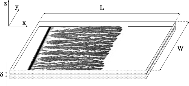
FIG. 1.: Schematic diagram of the thin-gap electrodeposition cell containing a ramified, metallic copper deposit. Note that the size of the deposit has been enlarged for clarity.

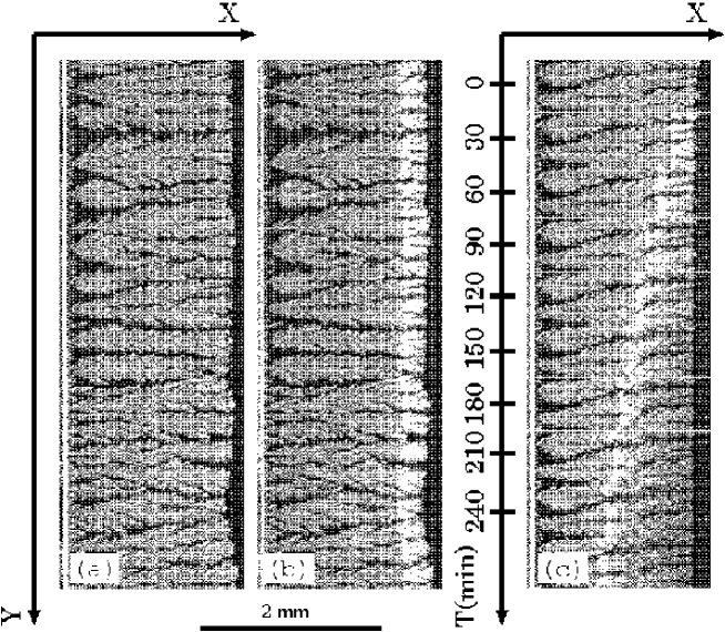
FIG. 2.: (a) Photograph of a copper deposit grown from a 0.5 mol.l^-1 CuCl₂ solution at $j$ = 40 mA.cm^-2 for approximately 15 minutes. (b) Photograph of the same deposit half an hour after the current had been switched off. (The white zone is CuCl.) (c) The montage shows a sequence of photographs of a small region of the deposit including the reaction front taken every 30 minutes after the interruption of the current.

FIG. 3.: Log-log plot of the position of the reaction front $X_{f}$ as a function of time $T$ for two different experimental runs in CuCl₂ 0.5 mol.l^-1 for deposits grown at $j=40$ mA.cm^-2. The solid lines of slope $\frac{1}{2}$ represent the predictions of the one-dimensional, mean-field theory, given by Eq. (41), with $D=10^{-5}$ cm².s^-1, in the cases $q=0.6$ and $q=0.73$.

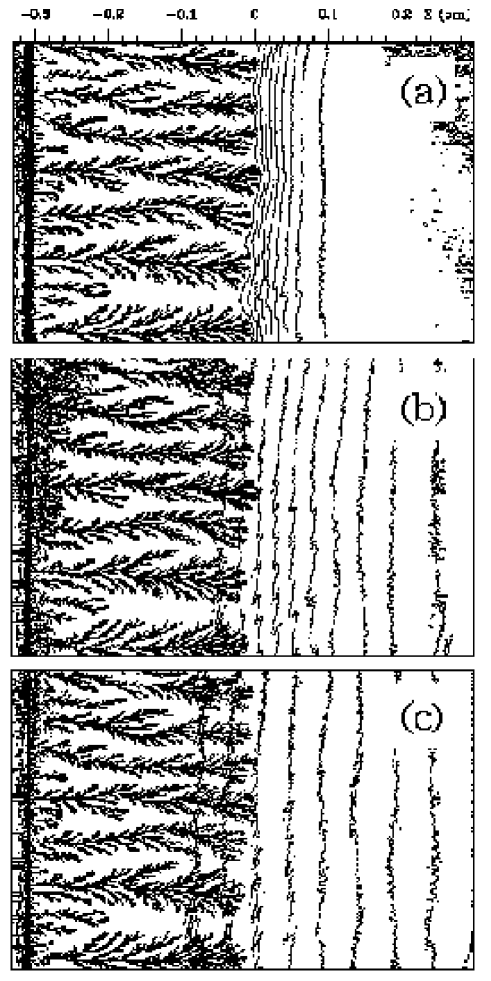
FIG. 4.: Interferometric characterization of the concentration field around a copper deposit during its dissolution (a) just before the interruption of the current, (b) 15 minutes and (c) one hour later. ($\Delta\rho\approx\rho_{A}^{o}/10$ between adjacent isoconcentration lines.) The deposit grown in 0.5 mol.l^-1 CuCl₂ solution at $j=40$ mA.cm^-2 for 20 minutes. The concentration of CuCl₂ is negligibly small inside and ahead (to the left) of the reaction front and approaches the bulk value of 0.5 mol.l^-1 far behind (to the right of) the front.

FIG. 5.: One-dimensional concentration profiles extracted from the two-dimensional data. The deposit has been grown from a 1 mol.l^-1 CuCl₂ solution at $j=68$ mA.cm^-2 during 15 minutes. The concentration profiles are shown every 15 minutes after the current had been switched off. The different symbols are added on each profile to differentiate the recording times. These symbols will be used on the next representations of the concentration profiles in Figs 9 and 10.

FIG. 6.: Log-log plot of the temporal evolution of the derivative of $a(X,T)$ at $X=0$ as a function of $T$. Same parameters as in Fig. 5. The plain line corresponds to the prediction of Eq. (45) with $D=10^{-5}$ cm².s^-1 and $q=0.79$.

FIG. 7.: The asymptotic similarity function $a(x,t)\sim A(\zeta)$ where $\zeta=\frac{x}{2\sqrt{t}}+\nu$ shown for $A_{o}=0$ and $\nu=$ 0, 0.5, 1, 1.5, 2, 2.5 from left to right.

FIG. 8.: The exact asymptotic dependence of $\nu$, the square root of the dimensionless diffusion constant of the reaction front, on the asymmetry parameter $q$, predicted by Eq. (39).

FIG. 9.: Collapse of the experimental concentration data in the diffusion layer plotted versus the similarity variable $(X-X_{f})/2\sqrt{DT}$ compared with the theoretically predicted asymptotic experimental similarity function $A(\zeta)$ (the solid line). The profiles are the same as those plotted in Fig. 5, but only one point out of 20 is shown on this plot for clarity.

FIG. 10.: Collapse of the experimental concentration data in the reaction front plotted versus the similarity variable $(X-X_{f})/2$. The solid line shows the linearized extension of the similarity function $A(\zeta)$ from the diffusion layer (see Fig. 9) extended into the reaction front. These profiles are the same as those plotted in Fig. 5, but only one point out of 4 is shown on this plot for clarity. The negative concentration values are artifacts of the interferometric technique and have no physical meaning.

FIG. 11.: Relaxation of the two dimensional initial concentration field at the beginning of the dissolution. (a) Isoconcentration line $a=0.1$, for $T=27$ s. The deposit has been grown from a 1 mol.l^-1 CuCl₂ solution, at $j=68$mA.cm^-2 during 15 minutes. (b) Log-linear plot of the evolution of the amplitude $G$ of the modulation of $A$ concentration, as shown in (a), versus the reduced time $T/\tau_{f}=4\nu^{2}DT/G(0)^{2}$.

REFERENCES

- [1] E. Jacob, Contemp. Phys. 34, 247 (1993), and references therein.
- [2] I. Epstein and K. Showalter, J. Phys. Chem. 100, 13132 (1996), and references therein.
- [3] E. Jacob, Contemp. Phys. 38, 205 (1997).
- [4] M. V. Smoluchowski, Phys. Z. 17, 557 (1916).
- [5] F. Collins and G. Kimball, J. of Colloid Science 4, 425 (1949).
- [6] D. Calef and J. Deutch, Ann. Rev. Phys. Chem. 34, 493 (1983).
- [7] L. Galfi and Z. Racz, Phys. Rev. Lett. 38, 3151 (1988).
- [8] A. Schenkel, P. Wittwer, and J. Stubbe, Physica D 69, 135 (1993).
- [9] Z. Koza, J. Stat. Phys. 85, 179 (1996).
- [10] M. Z. Bazant and H. A. Stone. (unpublished).
- [11] Z. Jiang and C. Ebner, Phys. Rev. A 42, 7483 (1990).
- [12] B. Choppard and M. Droz, Europhys. Lett. 15, 459 (1991).
- [13] S. Cornell, M. Droz, and B. Chopard, Phys. Rev. A 44, 4826 (1991).
- [14] S. Cornell, M. Droz, and B. Chopard, Physica A 188, 322 (1992).
- [15] S. Cornell and M. Droz, Phys. Rev. Lett. 70, 3824 (1993).
- [16] S. Cornell, Z. Koza, and M. Droz, Phys. Rev. E 52, 3500 (1995).
- [17] S. Cornell and M. Droz, Physica D 103, 348 (1997).
- [18] M. Araujo, H. Larralde, S. Havlin, and H. Stanley, Physica A 191, 168 (1992).
- [19] M. Araujo, H. Larralde, S. Havlin, and H. Stanley, Phys. Rev. Lett. 71, 3592 (1993).
- [20] Z. Koza and H. Taitelbaum, Phys. Rev. E (R) 54, 1040 (1996).
- [21] H. Taitelbaum, A. Yen, R. Kopelman, S. Havlin, and G. H. Weiss, Phys. Rev. E 54, 5942 (1996).
- [22] Y. Koo, L. Li, and R. Kopelman, Mol. Cryst. Liq. Cryst. 183, 187 (1990).
- [23] Y. L. Koo and R. Kopelman, J. Stat. Phys. 65, 893 (1991).
- [24] H. Taitelbaum, Y. L. Koo, S. Havlin, R. Kopelman, and G. Weiss, Phys. Rev. A 46, 2151 (1992).
- [25] H. Taitelbaum, B. Vilensky, A. Lin, Y.-E. L. Koo, and R. Kopelman, Phys. Rev. Lett. 77, 1640 (1996).
- [26] A. Yen, Y.-E. L. Koo, and R. Kopelman, Phys. Rev. E 54, 2447 (1996).
- [27] A. Yen, A. Lin, Y.-E. L. Koo, B. Vilensky, H. Taitelbaum, and R. Kopelman, J. Phys. Chem. A 101, 2819 (1997).
- [28] A. Yen and R. Kopelman, Phys. Rev. E 56, 3694 (1997).
- [29] A. Yen, Z.-Y. Shi, and R. Kopelman, Phys. Rev. E 57, 2438 (1998).
- [30] H. Taitelbaum and Z. Koza, Philosophical Magazine B 77, 1389 (1998).
- [31] Z. Koza, Physica A 240, 622 (1997).
- [32] S. Havlin, M. Araujo, Y. Lereah, H. Larralde, A. Shehter, H. Stanley, P. Trunfio, and B. Vilensky, Physica A 221, 1 (1995).
- [33] Data Translation frame grabber (768512) and public domain NIH Image program, developed at the U.S. National Institutes of Health and available on the Internet at http://rsb.info.nih.gov/nih-image/.
- [34] C. Léger, J. Elezgaray, and F. Argoul, Phys. Rev. Lett. 78, 5010 (1997).
- [35] K. Crennell, K. Gasvik, T. Yatagai, K. Creath, M. Kujawinska, D. Robinson, N. Halliwell, C. Pickering, and P. Hariharan, in Interferogram analysis, edited by D. Robinson and G. Reid (Institute of physics publishing, Techno House, Redcliffe Way, Bristol, BS1 6NX, England, 1993).
- [36] C. Léger, J. Elezgaray, and F. Argoul, Phys. Rev. E 58, 7700 (1998).
- [37] F. Oberholtzer, D. Barkey, and Q. Wu, Phys. Rev. E 57, 6955 (1998).
- [38] P. Trigueros, F. Sagues, and J. Claret, Phys. Rev. E 49, 4328 (1994).
- [39] M.-Q. Lòpez-Salvans, P. Trigueros, S. Vallmitjana, J. Claret, and F. Sagues, Phys. Rev. Lett. 76, 4062 (1996).
- [40] F. Texier, L. Servant, J. Bruneel, and F. Argoul, J. Electroanal. Chem 446, 189 (1998).
- [41] J. Newman, Electrochemical Systems (Prentice Hall, Englewood Cliff, New Jersey, 1991).
- [42] R. Parsons, Chem. Rev. 90, 813 (1980).
- [43] A. Bard and L. Faulkner, Electrochemical methods. Fundamentals and applications (John Wiley and Sons, New York, 1980).
- [44] J. Newman, Trans. Faraday Soc. 61, 2229 (1965).
- [45] J.-N. Chazalviel, Phys. Rev. A 42, 7355 (1990).
- [46] J. Elezgaray, C. Léger, and F. Argoul, J. Electrochem. Soc. 145, 2016 (1998).
- [47] J. Melrose, Phys. Rev. Lett. 65, 3009 (1990).
- [48] V. Fleury, J.-N. Chazalviel, M. Rosso, and B. Sapoval, J. Electroanal. Chem. 290, 249 (1990).
- [49] V. Fleury, M. Rosso, J.-N. Chazalviel, and B. Sapoval, Phys. Rev. A 44, 6693 (1991).
- [50] M. Z. Bazant, Phys. Rev. E 52, 1903 (1995).
- [51] A. Kuhn, F. Argoul, J. Muzy, and A. Arneodo, Phys. Rev. Lett. 73, 2998 (1994).
- [52] A. Kuhn and F. Argoul, J. Electroanal. Chem 397, 93 (1995).
- [53] F. Argoul, A. Arneodo, J. Elezgaray, and A. Kuhn, Fractals 5, 75 (1997).
- [54] B. Chopard, M. Droz, J. Magnin, and Z. Racz, Phys. Rev. E 56, 5343 (1997).
- [55] G. I. Barenblatt, Similarity, Self-Similarity and Intermediate Asymptotics (Cambridge University Press, Oxford, 1979).
- [56] J. Huth, H. Swinney, W. McCormick, A. Kuhn, and F. Argoul, Phys. Rev. E 51, 3444 (1995).
- [57] J.-N. Chazalviel, M. Rosso, E. Chassaing, and V. Fleury, J. Electroanal. Chem 407, 61 (1996).
- [58] E. Ben-Naim and S. Redner, J. Phys. A. Math. Gen. (L) 25, 575 (1992).
- [59] M. Abramowitz and I. A. Stegun, Handbook of Mathematical Functions (Dover, New York, 1965).
- [60] C. Bender and S. Orszag, Advanced Mathematical Methods for Scientists and Engineers (McGraw-Hill, New York, 1978).
- [61] B. Chopard, M. Droz, T. Karapiperis, and Z. Racz, Phys. Rev. E (R) 47, 40 (1993).
- [62] J. Krug and P. Meakin, Phys. Rev. Lett. 66, 703 (1991).