Evidence for a singularity in ideal magnetohydrodynamics: implications for fast reconnection        (Submitted to Phys. Rev. Lett. )

Abstract

Numerical evidence for a finite-time singularity in ideal 3D magnetohydrodynamics (MHD) is presented. The simulations start from two interlocking magnetic flux rings with no initial velocity. Curvature shrinks the rings until they touch and current sheets form between them. The evidence for a singularity in a finite time $t_{c}$ is that the peak current density behaves like $\|J\|_{\infty}\sim 1/(t_{c}-t)$ for a range of sound speeds and initial conditions. For the incompressible calculations $\|\mbox{\boldmath$\omega$}\|_{\infty}/\|{\bf J}\|_{\infty}\rightarrow\mbox{const}$. In resistive reconnection the magnetic helicity is nearly conserved while energy is dissipated.

To date it is not known whether or not the ideal magnetohydrodynamic (MHD) and Euler equations are regular. Regularity means that for arbitrary smooth initial data the velocity ${\bf u}$ and/or magnetic field ${\bf B}$ and all of its derivatives remain finite for all times. If regularity is not established, one cannot rule out the possibility of a finite time singularity, which for ideal MHD implies satisfying a new mathematical constraint that the vorticity $\mbox{\boldmath$\omega$}=\mbox{\boldmath$\nabla$}\times{\bf u}$ and current density ${\bf J}=\mbox{\boldmath$\nabla$}\times{\bf B}$ must obey [1]

$$I(t_{c})=\int_{0}^{t_{c}}\left[\|\mbox{\boldmath$\omega$}\|_{\infty}(t)+\|{\bf J}\|_{\infty}(t)\right]dt\rightarrow\infty,$$ (1)

for there to be a singularity. Singularities associated with shocks are also possible, but are not considered here, because they would not occur in the incompressible limit. The physical significance of a finite-time singularity is that fast vortex and/or magnetic field reconnection could be possible once viscous and resistive effects are restored. A theoretical demonstration of a mechanism for fast magnetic reconnection would be significant in a variety of problems in plasma physics including experimental studies related to magnetically confined fusion [2], dynamos, the earth’s magnetic field and the solar corona, where reconnection is associated with flares [3, 4] and coronal heating [5, 6]. This letter will show preliminary evidence for a possible singularity for ideal MHD using numerical simulations of three-dimensional linked magnetic flux rings and emphasize its relationship to fast magnetic reconnection.

Significant progress has been made recently for the Euler case where a numerical study of a pair of antiparallel vortex tubes has produced strong evidence for the formation of a singularity in the Euler equations in a finite time [7]. The numerical evidence was consistent with an analytic constraint for Euler [8] that no singularity can occur in a finite time $t=t_{c}$ in any quantity (e.g. in any derivative of ${\bf u}$, however high) unless

$$I(t_{c})=\int_{0}^{t_{c}}\|\mbox{\boldmath$\omega$}\|_{\infty}(t)dt\rightarrow\infty.$$ (2)

Here $\|...\|_{\infty}$ is the $L^{\infty}$ norm, or maximum, in space. This theorem shows that when searching for a singularity in the 3D Euler equations, the only quantity that needs to be monitored numerically is $\|\mbox{\boldmath$\omega$}\|_{\infty}$. Furthermore, if a singularity of the form $\|\mbox{\boldmath$\omega$}\|_{\infty}\sim(t_{c}-t)^{-\gamma}$ is observed in a numerical experiment then $\gamma$ must obey $\gamma\geq 1$ for the observed singular behavior to be genuine. The numerical comparisons [7] found $\gamma\equiv 1$, a scaling that is consistent dimensionally in addition to being consistent with (2). The generalization to MHD is (1).

An important feature of the analysis of the Euler calculations that should be used when analysing other flows with possible singularities is that singular behavior should be demonstrated by several independent tests. One set of tests predicted mathematically is that in addition to the $1/(t_{c}-t)^{\gamma}$ behavior of $\|\mbox{\boldmath$\omega$}\|_{\infty}$, all components of $\|\mbox{\boldmath$\nabla$}{\bf u}\|_{\infty}$ should diverge as $1/(t_{c}-t)^{\gamma}$ [9]. Again, $\gamma\equiv 1$ is expected. Another test that was found numerically [7] is that the rate of enstrophy production is

$$d\Omega/dt=\int\omega_{i}e_{ij}\omega_{j}\,dV\sim 1/(t_{c}-t)$$ (3)

where enstrophy is ${\textstyle{1\over 2}}\Omega=\int|\mbox{\boldmath$\omega$}|^{2}\,dV$.

The question of fast magnetic reconnection has been addressed using both time evolving calculations and steady-state analyses. In two-dimensional calculations, fast reconnection is inhibited by material that cannot escape easily from between thin current sheets. This led to early suggestions that a singularity in 2D MHD is precluded by the formation of current sheets [10] and is consistent with a recent result that there can be no singularity at 2D nulls [11]. New experimental evidence [2] designed to test two-dimensional steady-state theories shows a slow resistive timescale [12, 13, 14] instead of a faster timescale resulting from slow shocks [15] and related theories [16]. In three dimensions, the extra degree of freedom could allow material to escape more readily from the current sheets. This has prompted reconnection simulations in three dimensions, for example starting with orthogonal, straight flux tubes in pressure equilibrium and a small velocity field to push them together [17]. Explosive growth of $\|{\bf J}\|$ has been seen before [18], but not in the context of singularities.

We consider the equations for an isothermal, compressible gas for a given sound speed $c_{s}$ with a magnetic field of the form

$${\partial{\bf u}\over\partial t}=-{\bf u}\cdot\mbox{\boldmath$\nabla$}{\bf u}-c_{s}^{2}\mbox{\boldmath$\nabla$}\ln\rho+{{\bf J}\times{\bf B}\over\rho}+{\mu\over\rho}\left(\nabla^{2}{\bf u}+{\textstyle{1\over 3}}\mbox{\boldmath$\nabla$}\mbox{\boldmath$\nabla$}\cdot{\bf u}\right),$$

$${\partial\ln\rho\over\partial t}=-{\bf u}\cdot\mbox{\boldmath$\nabla$}\ln\rho-\mbox{\boldmath$\nabla$}\cdot{\bf u},$$ (4)

$${\partial{\bf A}\over\partial t}={\bf u}\times{\bf B}+\eta\nabla^{2}{\bf A},$$

where ${\bf B}=\mbox{\boldmath$\nabla$}\times{\bf A}$ is the magnetic field in terms of the magnetic vector potential ${\bf A}$, ${\bf u}$ is the velocity, and $\rho$ is the density. In the ideal limit, the resistivity $\eta$ and the viscosity $\mu$ are set to zero. The magnetic field is measured in units where the permeability is unity. Periodic boundary conditions are adopted in a domain of size $(2\pi)^{3}$. Our time unit is the sound travel time over a unit distance. The equations are advanced in time using a variable third-order Runge-Kutta timestep and sixth order explicit centered finite differences in space.

The equations for the incompressible case are the same except that the equation for $\rho$ is replaced by the divergence-free condition on velocity $\mbox{\boldmath$\nabla$}\cdot{\bf u}$ to determine the pressure. The magnetic field ${\bf B}$, rather than the vector potential ${\bf A}$, is used as a fundamental variable. The equations are advanced in time using a spectral colocation method with the 2/3-rule and variable third-order Runge-Kutta timestep. The maximum resolution used $384^{3}$ mesh points.

The incompressible, ideal MHD equations conserve total energy $E={1\over 2}\int({\bf u}^{2}+{\bf B}^{2})\,dV$, magnetic helicity $H_{B}=\int{\bf A}\cdot{\bf B}\,dV$ and the cross helicity $H_{C}=\int{\bf u}\cdot{\bf B}\,dV$. The helicities can be used to describe aspects of the topology [19]. Since $H_{B}$ has one less spatial derivative than the energy, spectrally it should dissipate more slowly than energy [20] when $\mu,\nu\neq 0$.

The initial conditions used in the present study will all be of two linked, magnetic flux rings. This condition is chosen because it has the advantage that no velocity field needs to be imposed in the initial conditions since the tension from the curvature of the rings induces a velocity by shrinking the rings. Due to the initial linkage, it also yields nearly maximal $H_{B}$ and therefore is an excellent choice for studying the dissipation of $H_{B}$ versus energy [19].

A variety of different ring thicknesses and angles between the initial rings have been investigated. This letter will discuss in detail only cases where the rings are orthogonal and are just touching. There are three distances that determine the initial condition that evolved into the structures in Figure 1: the radii of the rings $R$, the thickness $r_{\circ}$ where the flux goes smoothly to zero, and the separation of their centers from the origin $\Delta$. The separation of the rings is $2(R-\Delta)$. An initial profile across the ring that gives $|B|=1$ in the center and goes smoothly to $|B|=0$ at $r=r_{\circ}$ is taken from the Euler calculations [7]. $R=1$ and $\Delta=0.5$ for all the cases, so that they go through each other’s centers. The initial condition for the compressible calculations to be reported used $r_{\circ}=0.5$. $r_{\circ}=0.5$, 0.65 and 0.8 for the ideal incompressible cases. Following the example from the Euler case [7], the following hyperviscous filter was applied in Fourier space to the initial condition only: $\exp[-(k/k_{\max})^{4})$, where $k_{\max}$ is between 14 and 20. As a result, the maximum initial magnetic field $B_{0}$ is slightly less than one. For the compressible calculations, $c_{s}$ is varied between 0.1 and 10, so the initial plasma beta, $\beta_{0}=2c_{s}^{2}/B_{0}^{2}$, varied between 0.02 and 200. Only nearly incompressible $\beta_{0}=2$ calculations are presented. The initial density was uniform and unity. While what is being presented is nearly incompressible, preliminary low plasma beta calculations as well as compressible vortex reconnection [21] suggest that compressibility might enhance reconnection rates and singularity formation.

All of the compressible, resistive calculations were straightforward runs from $t=0$ with viscosities and resistivities chosen for a given resolution. The strategy for reaching the highest possible resolution for the ideal calculations followed the example of how a possible singularity in incompressible Euler was demonstrated [7]. First, the ideal calculations do not contain any numerical smoothing and have been run only so long as numerical dissipation was insignificant. This approach was used because experience has shown that artificial smoothing results in artificial dissipation which can obscure the dynamics of the ideal case. The lower resolution calculations were started from $t=0$. Since it would be too expensive to run higher resolution calculations from $t=0$, they are being remeshed at intermediate times.

There was no initial velocity field. The first, and shortest, phase after initialization was that due to the curvature of the flux rings their diameter $R$ shrinks. This automatically brings the flux tube rings into contact and the current of one ring begins to overlap the magnetic field of the other. This is necessary for the Lorentz force to be significant and for a strong interaction to begin.

To give an overall view of the flow, Figure 1 shows the three-dimensional structure from a $\beta=0.5$, $192^{3}$ resistive, compressible calculation, just before and after the estimated singular time. $t=2$ shows nearly ideal evolution from the initial motionless, perfectly tubular flux tubes. The dominant feature is the indentation in each ring. This is because in the cores of the flux rings the field is strongest and the magnetic curvature force largest. The region going singular appears in Figure 2a. as twisted current sheets within the center of Figure 1a. A surprising property of the reconnection process is that slices show that the size of the entire structure shrinks. Some perspective on this can be obtained by comparing the structures at $t=2$ and $t=3$.

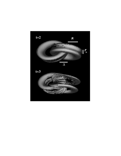
FIG. 1.: Resistive calculation using compressible code. $t=2$ shows evolution during the nearly ideal phase, $t=3$ shows a partially reconnected state with $H_{B}$ converted more into new twist between the remnants of the original tubes than into writhe within reconnected tubes.

By $t=3$ some reconnection has occurred. Magnetic helicity $H_{B}$ is nearly conserved, decreasing linearly at a very slow pace as it is converted into writhe [22] or new twist, and energy is dissipated more rapidly. A detailed examination of this structure will be studied elsewhere.

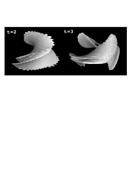
FIG. 2.: Three-dimensional level surfaces of the magnitude of the current density in the resistive calculation. $t=2$ shows a double saddle surface, which at $t=3$ is broken up into two disjoint pieces.

In a resistive calculation, the dissipation is concentrated on a current sheet that forms where the two flux rings come into contact. Level surfaces of the current density near its peak value (Fig. 2) show a twisted, saddle shaped, double-sheet structure before the estimated singular time, which separates into two disjoint sheets centered around the points of maximum current density after the singular time.

Figure 3 shows $1/\|{\bf J}\|_{\infty}$ and $1/(\|{\bf J}\|_{\infty}+\|\mbox{\boldmath$\omega$}\|_{\infty})$ for the resistive calculations. There is a strong tendency in favor of linear behavior similar to that observed for 3D Euler [7]. Extrapolating from before $t=2.3$ to $1/J_{\max}=0$ suggests that $t_{c}\approx 2.5$. For $c_{s}>0.5$, that is more incompressible, roughly the same singular time would be predicted. For $c_{s}<.5$, that is more compressible, different behavior is indicated, but the trend toward $1/\|{\bf J}\|_{\infty}\sim(t_{c}-t)$ remains.

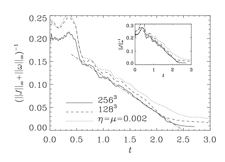
FIG. 3.: Evolution of $1/\|{\bf J}\|_{\infty}$ and $1/(\|{\bf J}\|_{\infty}+\|\omega\|_{\infty})$. $r=0.5$ for $\beta_{0}=2$. Solid and dashed lines refer to ideal calculations with different resolution and the dotted line is for a resistive calculation with $\eta=\mu=0.002$. The dash-dotted line gives a linear fit to the data.

For Euler, recall that stronger evidence for a possible singularity was obtained by monitoring the $L^{\infty}$ norm for an additional strain term and the enstrophy production, as well as $\|\mbox{\boldmath$\omega$}\|_{\infty}$ [7]. Following that reasoning, we need to know the behavior of two first derivatives of the magnetic or velocity fields plus a global production term. Therefore, we propose looking at the behavior of $\|{\bf J}\|_{\infty}$, $\|\mbox{\boldmath$\omega$}\|_{\infty}$, and the production of $\Omega_{\omega+J}={\textstyle{1\over 2}}\int(|\mbox{\boldmath$\omega$}|^{2}+|{\bf J}|^{2})\,dV$,

$$P_{\Omega J}=\int(\omega_{i}e_{ij}\omega_{j}-\omega_{i}d_{ij}J_{j}+2\varepsilon_{ijk}J_{i}d_{j{\ell}}e_{{\ell}k})\,dV,$$ (5)

where $e_{ij}={1\over 2}(u_{i,j}+u_{j,i})$ and $d_{ij}={1\over 2}(B_{i,j}+B_{j,i})$ are the hydrodynamic and magnetic strains. The terms in $P_{\Omega J}$, in order, are the vortex stretching already known for Euler, a new vorticity production term and a new current producing term. All three tests should go as $1/(t_{c}-t)$ once sufficiently singular solutions are obtained, which we have not yet achieved. Therefore, the present objective is trends in the right direction, rather than conclusive evidence for the existence of a singularity.

Figure 4 plots the three proposed tests for the $r_{\circ}=0.65$ incompressible case. The $384^{3}$ run was used for the $1/\|{\bf J}\|_{\infty}$ and $1/\|\mbox{\boldmath$\omega$}\|_{\infty}$ tests for $t>1$ and the $192^{3}$ run for $1/P_{\Omega J}$ for all time.

FIG. 4.: Comparison of the evolution of $1/\|{\bf J}\|_{\infty}$, $1/\|\mbox{\boldmath$\omega$}\|_{\infty}$ and $P_{\Omega J}$ for $r_{\circ}=0.65$. The inset shows $\|\mbox{\boldmath$\omega$}\|_{\infty}/\|{\bf J}\|_{\infty}$ for $r=$0.5, 0.65 and 0.8, all of which are converging to $\|\mbox{\boldmath$\omega$}\|_{\infty}/\|{\bf J}\|_{\infty}\approx 0.5$, demonstrating possible self-similarity.

In the case of Euler it was shown that ratios of all $L^{\infty}$ norms of first derivatives were approaching constant values [7], which would be consistent with self-similar behavior near the point going singular. Therefore we expect that $\|\mbox{\boldmath$\omega$}\|_{\infty}/\|{\bf J}\|_{\infty}$ should approach a constant value here. Initially the velocity, and vorticity, are zero, so these must build up before behavior for $\|\mbox{\boldmath$\omega$}\|_{\infty}$ and $P_{\Omega J}$ consistent with $1/(t_{c}-t)$ appears. The inset in Figure 4 shows that all three cases appear to be converging to a value of $\|\mbox{\boldmath$\omega$}\|_{\infty}/\|{\bf J}\|_{\infty}\approx 0.5$. $r_{\circ}=0.65$ converges the soonest, near $t=1.6$ and together with the convergence of $\|\mbox{\boldmath$\omega$}\|_{\infty}/\|{\bf J}\|_{\infty}\rightarrow 0.5$ is our best evidence to date for a possible singularity in ideal MHD. In addition, $1/P_{\Omega J}$ appears to join the same $(t_{c}-t)$ near $t=1.9$.

While $1/\|{\bf J}\|_{\infty}$ for the $r_{\circ}=0.5$ incompressible case is comparable to the compressible case and shows the largest range of $1/\|{\bf J}\|_{\infty}\sim(t_{c}-t)$ behavior, it is not strong evidence for a singularity because the inset in Figure 4 shows that its $1/\|\mbox{\boldmath$\omega$}\|_{\infty}$ up to $t=2.0$ does not have the same value for $t_{c}$. However, note that the production term for ${\bf J}^{2}$ in (5), $2\varepsilon_{ijk}J_{i}d_{j{\ell}}e_{{\ell}k}$, does not involve vorticity, but only strain terms. Unlike Euler, vorticity seems to be playing only a secondary role for ideal MHD. It is not essential for vorticity to blow up for the compressible cases, and it does not. Related to this, the current sheets near $\|{\bf J}\|_{\infty}$ in Figure 2 are twisted. This also suggests that similar hydrodynamic initial conditions should be revisited to determine their reconnection rates [23]. Further analysis of local production terms in proposed $600^{3}$ calculations should help answer these questions.

In conclusion, we have presented numerical evidence for a finite-time blow-up of the current density in ideal MHD in the case of interlocked magnetic flux rings. In the resistive case one would not expect there to be a singularity. Instead, arbitrarily thin current sheets will form, depending on how small the resistivity is [24]. This can lead to significant dissipation whose strength is virtually independent of resistivity. The astrophysical significance of current sheets as a consequence of tangential discontinuities of the field has also been stressed in a recent book by Parker [5]. However, the possibility of a finite time singularity in ideal MHD is not commonly discussed in connection with fast reconnection.

This work has been supported in part by an EPSRC visiting grant GR/M46136. NCAR is support by the National Science Foundation. We appreciate suggestions by J.D. Gibbon, I. Klapper, and H.K. Moffatt.

REFERENCES

- [1] R. E. Caflisch, I. Klapper, and G. Steele, Comm. Math. Phys. 184, 443 (1997).
- [2] M. Yamada et al. Phys. Plasmas 4, 1936 (1997).
- [3] M. Ohyama and K. Shibata, Publ. Astron. Soc. Japan 49, 249 (1997).
- [4] Y. Ogawara et al. Publ. Astron. Soc. Japan 44, L41 (1992). (and references therein)
- [5] E. N. Parker, Spontaneous current sheets in magnetic fields (Oxford University Press, New York, 1994), pp. 225.
- [6] K. Galsgaard and Å. Nordlund J. Geophys. Res. 101, 13445 (1996).
- [7] R. M. Kerr, Phys. Fluids 5, 1725 (1993).
- [8] J. T. Beale, T. Kato, and A. Majda, Comm. Math. Phys. 94, 61 (1984).
- [9] G. Ponce, Comm. Math. Phys. 98, 349 (1985).
- [10] P. L. Sulem, et al., J. Plasma Phys. 33, 191 (1985).
- [11] I. Klapper, Phys. Plasmas 5, 910, (1998).
- [12] P. A. Sweet, Nuovo Cimento Suppl. 8, Ser, X, 188 (1958).
- [13] E. N. Parker, J. Geophys. Res. 4, 509 (1957).
- [14] E. N. Parker, Astrophys. J. Suppl. 77, 177, (1963).
- [15] H. E. Petschek, in: Symposium on the Physics of Solar Flares, edited by W. N. Hess (NASA, Washington, D.C, 1964), pp. 425.
- [16] E. R. Priest and T. G. Forbes, J. Geophys. Res. 97, 16757 (1992).
- [17] R. B. Dahlburg and S. K. Antiochos, J. Geophys. Res. 100, 16,991 (1995).
- [18] H. Baty, G. Einaudi, R. Lionello and M. Velli, Astron. Astrophys. 333, 313 (1998).
- [19] H. K. Moffatt, J. Fluid Mech. 35, 117 (1969).
- [20] M. Berger, Geophys. Astrophys. Fluid Dyn. 30, 79 (1984).
- [21] D. Virk, F. Hussain and R. M. Kerr, J. Fluid Mech. 304, 17 (1995).
- [22] H. K. Moffatt and R. L. Ricca, Proc. Roy. Soc. Lond. A 439, 411 (1992).
- [23] H. Aref and I. Zawadzki, Nature 354, 50 (1991).
- [24] A. Otto, J. Geophys. Res. 100, 11863 (1995).