Lifetimes of agents under external stress

Abstract

An exact formula for the distribution of lifetimes in coherent-noise models and related models is derived. For certain stress distributions, this formula can be analytically evaluated and yields simple closed expressions. For those types of stress for which a closed expression is not available, a numerical evaluation can be done in a straightforward way. All results obtained are in perfect agreement with numerical experiments. The implications for the coherent-noise models’ application to macroevolution are discussed.

Agents under externally imposed stress have been recently studied in coherent-noise and related models [1, 2, 3, 4, 5, 6, 7]. These models display scale free distributions in a number of quantities, such as event sizes and lifetimes, or in the decay pattern of aftershocks. Coherent-noise models are very different from other models displaying scale free behavior, such as sand pile models [8], as they do not rely on local interactions or feedback. Hence, they are not self organized critical. Considered the abundance of power-law distributed quantities in nature [9], models such as the ones of the coherent-noise type can help understanding to what extent self-organized criticality is the right paradigm for describing driven systems, and to what extent other mechanisms can provoke similar power-law distributions.

Despite the simplicity of the original coherent-noise model—agents have thresholds $x_{i}$; if global stress exceeds a threshold $x_{i}$, agent $i$ gets replaced; with prob. $f$, an agent gets a new threshold—, no exact analytical results have been obtained so far. The distributions of event sizes and aftershocks have been studied in detail in [3] (event sizes) and in [10] (aftershocks). Both distributions can be regarded as being well understood. Nevertheless, the theoretical results are only of approximative character in both cases.

In the case of the distribution of lifetimes, there are even less theoretical results. Sneppen and Newman [3] have given an expression based on their time-averaged approximation. This expression is right for certain stress distributions, as we will show below. However, it breaks down for slowly decaying distributions such as the Lorentzian distribution. Moreover, it is not clear when exactly it can be applied.

In a recent paper [7], a different approach of calculating the distribution of lifetimes has been taken, and the author claimed that the lifetimes obey multiscaling, with a $L^{-2}$ decrease for small lifetimes, and a $L^{-1}$ decrease for large lifetimes. Here, we will demonstrate that this statement is wrong. We will calculate the distribution of lifetimes exactly, without any approximations, and we will show that our results are in perfect agreement with numerical simulations.

Our calculations are based on the observation that it is not necessary to know the distribution of thresholds $\rho(x)$ for calculating the distribution of lifetimes. All we have to know is the distribution according to which agents enter the system, which is called $p_{\rm thresh}(x)$ in the notation of [1], and the stress distribution $p_{\rm stress}(x)$. Once an agent has entered the system, it has a well defined life expectancy, which is closely related to the probability that the agent will be hit by stress or mutation. Note that in this picture, we are considering only a single agent. Therefore, if we talk about lifetimes, it does not matter whether the stress acts coherently on a large number of agents, or whether it is drawn for all agents independently. In this respect, the results we obtain in this work are of a much more general nature than the results found previously for event sizes or aftershocks.

An agent with threshold $x$ will survive stress and mutation in one time step with a probability $p(x)$ equal to [5]

$$p(x) = (1-f)[1-p_{\rm move}(x)]$$ (1)

$$= (1-f)\int_{0}^{x}p_{\rm stress}(x^{\prime})\,dx^{\prime}\,.$$ (2)

What is the distribution of the survival probabilities $p$? We denote the corresponding density function by $u(p)$. Clearly, we have

$$u(p)\,dp = p_{\rm thresh}(x)\,dx$$ (3)

$$= dx\quad\mbox{for}\quad 0\leq x<1\,.$$ (4)

In the second step, we have assumed that the threshold distribution is uniform. This can always be achieved after a suitable transformation of variables [3]. Hence, we find

$$u(p)=\frac{dx}{dp}\,.$$ (5)

The derivative $dx/dp$ can be calculated from Eq. (1),

$$\frac{dx}{dp}=\frac{1}{(1-f)p_{\rm stress}[x(p)]}\,,$$ (6)

and $x(p)$ can be obtained from Eq. (1) by inversion. The density function is thus defined for $p<p_{\max}$, where

$$p_{\max}=p(1)=(1-f)\int_{0}^{1}p_{\rm stress}(x)\,dx$$ (7)

stems from the condition that the thresholds are distributed uniformly between 0 and 1. Above $p_{\max}$, the density function $u(p)$ is equal to zero.

All agents with the same survival probability $p$ generate a distribution of lifetimes which reads

$$g(L)=p^{L-1}(1-p)\,.$$ (8)

Here, $g(L)$ is the probability density function for the lifetimes $L$. Note that the model works in discrete time steps, therefore the lifetimes $L$ are integers, and $g(L)$ is only defined for integral arguments. We can calculate the distribution of lifetimes $h(L)$ by averaging over the distributions generated by different survival probabilities $p$, weighted with their density function $u(p)$:

$$h(L)=\int_{0}^{p_{\max}}u(p)p^{L-1}(1-p)\,dp\,.$$ (9)

Equation (9) can be explicitly evaluated for exponentially distributed stress, $p_{\rm stress}=\exp(-x/\sigma)/\sigma$. We find

$$u(p)=\frac{\sigma}{1-f-p}\quad\mbox{for}\quad 0\leq p<p_{\max}\,,$$ (10)

with

$$p_{\max}=(1-f)[1-\exp(-1/\sigma)]\,.$$ (11)

After inserting this into Eq. (9) and doing some basic calculations, we obtain

$$h(L)=\frac{\sigma p_{\max}^{L}}{L}+f\sigma\int_{0}^{p_{\max}}\frac{p^{L-1}}{1-f-p}\,dp\,.$$ (12)

It is possible to calculate the remaining integral with the aid of the identity (see [11], 15.3.1)

$$\int_{0}^{1}t^{b-1}(1-t)^{c-b-1}(1-tz)^{-a}\,dt=$$ (13)

$$\qquad\qquad\qquad=\frac{\Gamma(b)\Gamma(c-b)}{\Gamma(c)}F(a,b;c;z)\,,$$ (14)

where $F(a,b;c;z)$ is the hypergeometric function. We find

$$h(L)=\sigma\frac{p_{\max}^{L}}{L}\left[1+\frac{f}{1-f}F\left(L,1;L+1;\frac{p_{\max}}{1-f}\right)\right]\,.$$ (15)

The leading term $\sigma p_{\max}^{L}/L$ is responsible for a $L^{-1}$ decay with cut off at $L\approx 1/f$. This behavior has been reported previously, and it corresponds to the approximation derived in [3]. The correcting term vanishes with $f$. It is of importance only for extremely long lifetimes of the order $1/f$, for which it modifies the detailed cut off behavior.

In Fig. 1 we display Eq. (15) together with results from direct numerical simulations, for different values of $f$. The theoretical result is in perfect agreement with the measured distributions. The dependency of the cut off on $f$ is clearly visible in Fig. 1.

Another stress distribution for which we can derive a closed analytic form for $h(L)$ is the uniform distribution, $p_{\rm stress}(x)=1$ for $0\leq x<1$. We find

$$u(p)=\frac{1}{1-f}\quad\mbox{for}\quad 0\leq p<1-f$$ (16)

and

$$h(L)=\frac{(1-f)^{L-1}}{L(L+1)}(1+fL)\,.$$ (17)

As in the case of Eq. (12), we get a leading and a correcting term. The leading term decays as $L^{-2}$ with cut-off at $L\approx 1/f$, and the second term modifies the cut-off behavior. Interestingly, the distribution of lifetimes is scale-free, although the distribution of event sizes in a coherent-noise model with uniform stresses is not a power law [3]. A plot of Eq. (17) is given in Fig. 2, together with the corresponding measured distribution.

For the most other stress distributions, the integral in Eq. (9) can only be done numerically. This is the case, for example, for the Gaussian distribution, $p_{\rm stress}(x)=\sqrt{2/(\pi\sigma^{2})}\exp[-x^{2}/(2\sigma^{2})]$. Under Gaussian stress, an agent with threshold $x$ will survive a single time step with probability

$$p(x)=(1-f)\,{\rm erf}\left(\frac{x}{\sqrt{2}\sigma}\right)\,,$$ (18)

where ${\rm erf}(x)$ is the error function

$${\rm erf}(x)=\frac{2}{\sqrt{\pi}}\int_{0}^{x}\exp(-t^{2})\,dt\,.$$ (19)

Inversion of Eq. (18) yields

$$x(p)=\sqrt{2}\sigma\,{\rm erf}^{-1}\left(\frac{p}{1-f}\right)\,.$$ (20)

Here, by ${\rm erf}^{-1}(z)$ we denote the inverse error function, obtained by solving the equation $z={\rm erf}(x)$ for $x$. We can calculate the density function of the survival probabilities with the aid of Eqs. (6) and (20). The resulting expression reads

$$u(p)=\sqrt{\frac{\pi}{2}}\frac{\sigma}{1-f}\exp\left(\left[{\rm erf}^{-1}\left(\frac{p}{1-f}\right)\right]^{2}\right)\,.$$ (21)

The numerical integration of $u(p)p^{L-1}(1-p)$ is somewhat tricky for choices of $\sigma$ such, that $p_{\max}/(1-f)$ is very close to 1, since the inverse error function has a singularity at 1. However, for moderately small $\sigma$, the integration can be carried out without too much trouble. The resulting density function $h(L)$ is shown in Fig. 2 for $\sigma=0.15$ and $f=10^{-4}$. We find that, for $L\ll 1/f$, the function $h(L)$ is almost linear in the log-log plot. A fit to the linear region of $h(L)$ gives an exponent $\tau=1.177\pm 0.01$, which means $h(L)$ decays slightly steeper than the $L^{-1}$ decay predicted by the approximation of Sneppen and Newman. However, if we evaluate $h(L)$ for much larger $L$ and much smaller $f$, we find that the exponent $\tau$ decreases slowly towards the value 1 (Fig. 3).

Let us now turn to the Lorentzian distribution $p_{\rm stress}(x)=(2a/\pi)/(x^{2}+a^{2})$. In this case, a calculation along the lines of Eqs. (1)–(7) yields the following distribution of survival probabilities:

$$u(p)=\frac{\pi}{2}\frac{a}{1-f}\left(\cos^{2}\left[\frac{\pi}{2}\frac{p}{1-f}\right]\right)^{-1}\,.$$ (22)

Here, $p_{\rm max}=(2/\pi)(1-f)\arctan(1/a)$. The result of the numerical integration is shown in Fig. 4. As in the previous cases, we observe a perfect agreement between the analytic expression for $h(L)$ and the distribution measured in computer experiments. In the case of Lorentzian stresses, the distribution of lifetimes is clearly not scale invariant.

In [7] it has been claimed that the distribution of the agents’ lifetimes under external stress decays as $L^{-2}$ for small $L$. Among the four stress distributions considered in this work, we found a $L^{-2}$ decay only for the uniform stress distribution. Hence the statement made in [7] is wrong in general. We could verify the $L^{-1}$ decay reported in [3] for exponential or Gaussian stresses. As it was also stated there, the Lorentzian stress distribution does not produce a scale free distribution of lifetimes.

A surprising result of this work is the observation that the properties of the distribution of lifetimes and of the distribution of event sizes in a coherent-noise model are largely independent from each other. We do find power-law distributed lifetimes under uniform stress, under which the distribution of event sizes is not scale free, and we do not find power-law distributed lifetimes under Lorentzian stress, which generates a scale free distribution of event sizes. Consequently, we cannot infer from a power-law distribution of event sizes to one of lifetimes, and vice versa. Both distributions have to be investigated independently for every type of stress.

Let us conclude with some remarks on the implications of our results for the application of coherent-noise or related models to large scale evolution. In the context of macroevolution, the agents are regarded as species, or higher taxonomical units, such as genera or families [12]. The distribution of genus lifetimes in the fossil record follows either a power-law decrease with exponent near 2, or an exponential decrease [13, 14]. A $L^{-2}$ decay can be observed in coherent-noise models with uniform stress. However, in this case the distribution of extinction events does not follow the $s^{-2}$ decay – with $s$ denoting the number of families gone extinct in one time step – found in the fossil record [2]. The distribution of lifetimes closest to an exponential decay is, among the stress distributions we studied here, generated by Lorentzian stresses. But also in this case, the distribution of extinction events is significantly different from the needed $s^{-2}$ decay of extinction events. On the other hand, it seems to be typical for distributions generating a $s^{-2}$ decay, such as exponential, Gaussian, or Poissonian, that the distribution of lifetimes decays as $L^{-1}$. It is arguable whether any type of stress can actually generate the right type of distribution for lifetimes and extinction events simultaneously. Hence, the coherent-noise models in their current formulation probably miss some important ingredient as a model of macroevolution. An effect which is not covered, and which has been shown recently to be of importance for the statistical patterns in the fossil record, is a decline in the extinction rate [14, 15, 16, 17]. For example, Sibani et al. [16, 18] have demonstrated that the $L^{-2}$ decay in lifetimes might be closely related to the decline in the extinction rate.

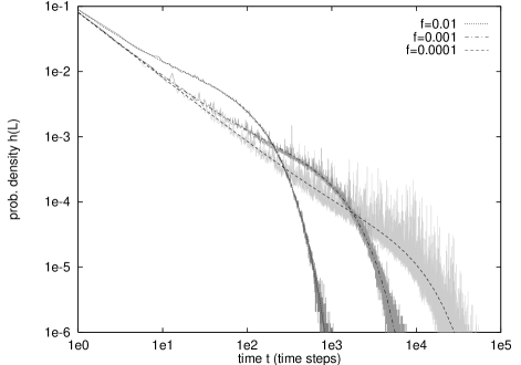
FIG. 1.: The distribution of lifetimes of agents subjected to exponentially distributed stress, with $\sigma=0.08$. The gray lines represent the results obtained from computer experiments, the black lines represent the theoretical prediction Eq. (12). Theory and computer experiment are in perfect agreement.

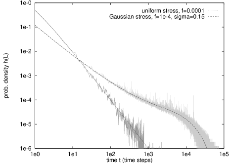
FIG. 2.: Comparison of theory and computer experiment for the uniform and for the Gaussian stress distribution. As in the case of Fig. 1, we observe perfect agreement.

FIG. 3.: The distribution of lifetimes of agents under Gaussian stress, with $\sigma=0.15$ and different values of $f$. For very small mutation rates $f$, the distribution of lifetimes becomes $1/L$ for $L$ larger than about $10^{5}$ time steps.

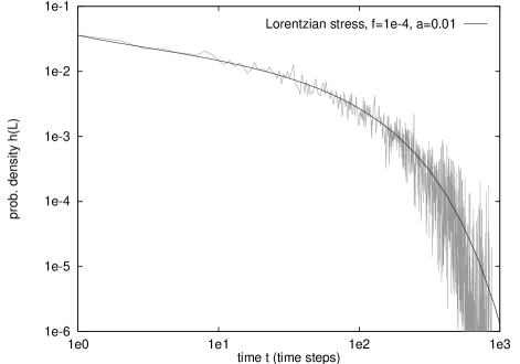
FIG. 4.: With Lorentzian stresses, the distribution of lifetimes is no longer scale invariant.

REFERENCES

- [1] M. E. J. Newman and K. Sneppen, Phys. Rev. E 54, 6226 (1996).
- [2] M. E. J. Newman, Proc. R. Soc. London B 263, 1605 (1996).
- [3] K. Sneppen and M. E. J. Newman, Physica D 110, 209 (1997).
- [4] C. Wilke and T. Martinetz, Phys. Rev. E 56, 7128 (1997).
- [5] C. Wilke, S. Altmeyer, and T. Martinetz, Physica D 120, 401 (1998).
- [6] C. Wilke and T. Martinetz, Phys. Rev. E 58, 7101 (1998).
- [7] R. K. Standish, Phys. Rev. E in press (1999), eprint physics/9806046.
- [8] P. Bak, C. Tang, and K. Wiesenfeld, Phys. Rev. Lett. 59, 381 (1987).
- [9] P. Bak, How nature works (Springer-Verlag, New York, 1997).
- [10] C. Wilke, S. Altmeyer, and T. Martinetz, in Proc. of “Artificial Life VI”, edited by C. Adami, R. Belew, H. Kitano, and C. Taylor (MIT Press, Cambridge, MA, 1998), pp. 266–272.
- [11] Pocketbook of mathematical functions, edited by M. Abramowitz and I. A. Stegun (Harri Deutsch Verlag, Thun; Frankfurt/Main, 1984).
- [12] M. E. J. Newman, J. theor. Biol. 189, 235 (1998).
- [13] K. Sneppen, P. Bak, H. Flyvbjerg, and M. H. Jensen, Proc. Natl. Acad. Sci. USA 92, 5209 (1995).
- [14] M. E. J. Newman and P. Sibani, Proc. R. Soc. London B, submitted (1998), eprint adap-org/9811003.
- [15] D. M. Raup and J. J. Sepkoski, Jr., Science 215, 1501 (1982).
- [16] P. Sibani, M. R. Schmidt, and P. Alstrøm, Phys. Rev. Lett. 75, 2055 (1995).
- [17] M. E. J. Newman and G. J. Eble, Paleobiology, submitted (1998), eprint adap-org/9809004.
- [18] P. Sibani, Phys. Rev. Lett. 79, 1413 (1997).