Time-dependent control of ultracold atoms and Bose-Einstein condensates in magnetic traps

Abstract

With radiofrequency fields one can control ultracold atoms in magnetic traps. These fields couple the atomic spin states, and are used in evaporative cooling which can lead to Bose-Einstein condensation in the atom cloud. Also, they can be used in controlled release of the condensate from the trap, thus providing output couplers for atom lasers. In this paper we show that the time-dependent multistate models for these processes have exact solutions which are polynomials of the solutions of the corresponding two-state models. This allows simple, in many cases analytic descriptions for the time-dependent control of the magnetically trapped ultracold atoms.

Neutral atoms possessing hyperfine structure can be trapped in spatially inhomogeneous magnetic fields, if they are in the appropriate spin state. As the magnetic field imposes spin-dependent Zeeman shifts on the atomic energy levels, a spatially changing magnetic field maps into an external potential felt by the atom (see Fig. 1). The magnetic traps are, however, very shallow, so only ultracold atoms can be trapped. For alkali atoms the proper temperatures have been obtained via precooling with laser light. Once the atoms are trapped, one can decrease the trap depth, which allows the hot atoms to escape, and those left behind thermalize via collisions into a lower temperature—this is called evaporative cooling [1]. By combining magnetic traps with evaporative cooling one can now reach the densities and temperatures where Bose-Einstein condensation takes place [2]. Then the atoms form a coherent superposition, which can be released from the trap [3]. As the escaping atoms maintain their coherence [4], the experiment is a prototype for an atom laser, i.e., production of coherent, propagating packets of matter waves.

FIG. 1.: Magnetic trapping of neutral atoms. We show the atomic potentials for the $f=1$ trapping system, and how the radiofrequency field (frequency $\omega_{\rm rf}$) can be used to control the trap depth $k_{B}T_{d}$. The resonant transition $m=-1\rightarrow m=0\rightarrow m=+1$ moves the atoms with kinetic energy larger than $k_{B}T_{d}$ from the trapping state to a strongly nontrapping state.

Evaporative cooling requires effective and precise control of the trap depth. This can be achieved by coupling the spin states (labeled with the magnetic quantum number $m$) with a radiofrequency (rf) field [1, 5, 6]. The coupling introduces transitions between the neighbouring spin states ($\Delta m=\pm 1$). As demonstrated in Fig. 1, the frequency $\omega_{\rm rf}$ of the field controls the depth of the trap. If we want to estimate the efficiency of evaporative cooling, we can transform the rf resonances into curve crossings, and describe the dynamics of the atoms at the edge of the trap with an appropriate time-dependent curve crossing model [1], see Fig. 2. Typically one compares the trap oscillation period times the spin-change probability at the resonance point to the other time scales of the trapping and cooling process, including collisional loss rates [1].

However, as one usually operates in the region where Zeeman shifts are linear, the rf field couples sequentially all spin states, instead of just selecting a certain pair of states. In case of only two spin states we can use the standard Landau-Zener model in estimates of the efficiency of evaporative cooling. In practice, however, one has $2f+1$ states, where $f$ is the hyperfine quantum number of the atomic state used for trapping. So far condensates have been realised for $f=1$ and $f=2$, but experiments e.g. with cesium involve states with $f=3$ and $f=4$, so in order to achieve efficient evaporative cooling one needs several sequential rf-induced transitions. Clearly the use of the two-state Landau-Zener model can be questioned in these multistate cases.

Once the Bose-Einstein condensation has been achieved one can release the condensate just by switching the magnetic field off. This technique, however, does not allow much control over the release. Moreover, it always involves all the atoms. With rf fields one can transform parts of the condensate into untrapped states, in which they are typically accelerated away—this has been demonstrated experimentally [3], as well as the fact that the released atoms are in a coherent superposition [4], thus justifying the term “atom laser”. This output coupling process can be achieved either by using rf pulses which are resonant at the trap center, or by using chirped rf fields. Both correspond to a multistate Hamiltonian, where either the diagonal terms (chirping) or the off-diagonal terms (rf pulses) have explicit time dependence. In Ref. [3] the output coupling process was demonstrated experimentally for the sodium $f=1$ situation, and the transition probabilities were in good agreement with the predictions of time-dependent three-state models.

Both evaporative cooling and output coupling demonstrate the need to have analytic solutions for the time-dependent multistate models of the rf-induced dynamics. Although these models can be easily solved numerically, they are often used only as a part of a bigger theoretical description, in which the dependence of the solutions on the parameters such as the frequency and intensity of the rf field, or chirp parameters and shapes of pulse envelopes are required. Instead of looking into the known effects of rf fields, we can consider the effects first, and then look how we need to tailor the rf field in order to achieve what we want—in this approach the analytic models show clearly their supremacy. Furthermore, as we show in this Letter, the description of the rf-induced multistate processes is closely connected to the two-state processes, which means that the wealth of knowledge on two-state models that has been accumulated in the past [7, 8] can be applied—and tested—with Bose-Einstein condensates.

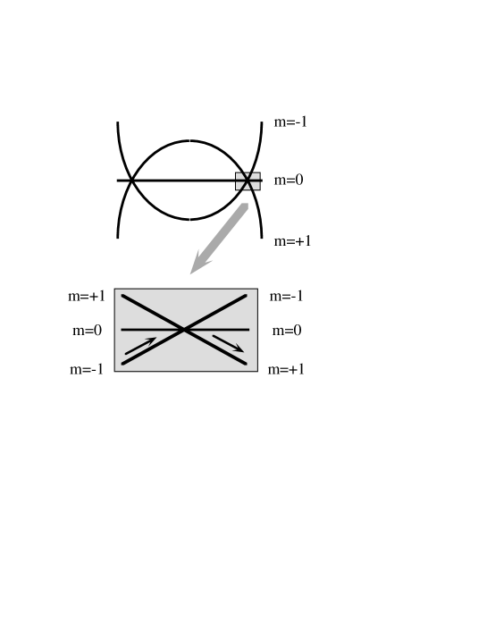
FIG. 2.: The curve crossing description of trap dynamics. The potentials are obtained by shifting the atomic states by multiples of rf photon energies. The region near the resonance point can be modelled with a bowtie crossing as shown in the enlargement of the grey area. Assuming that an atom traverses the crossing with some constant velocity $v_{c}$, we can map the position-dependent crossing into a time-dependent one, which in the special case of two states corresponds to the widely used and well-known Landau-Zener model. In the optimal, i.e., adiabatic case the hot atoms follow the route marked by arrows out of the trap.

First we need to derive the Hamiltonian describing the rf-induced processes. The field ${\bf B}=B_{0}\cos(\omega_{\rm rf}t){\bf e}_{\rm rf}$ couples to the atomic magnetic moment $\boldmath\mu$, i.e., $H_{\rm int}=-\mbox{\boldmath$\mu$}\cdot{\bf B}$. The matrix elements of this coupling between the magnetic states of the same hyperfine manifold are nonzero only if $\Delta m=\pm 1$. Furthermore, using the angular momentum algebra we see that the couplings between neighbouring states have the form [1, 9]

$$H_{m,m+1}=H_{m+1,m}=\sqrt{(f-m)(f+m+1)}\hbar\Omega,$$ (1)

where $\Omega$ is the Rabi frequency quantifying the coupling. Here we have applied the rotating wave approximation and eliminated the field terms oscillating with frequency $\omega_{\rm rf}$. This leads to the curve crossing picture of the atomic potentials [8].

In the regime of the linear Zeeman effect the energy difference between two neighbouring $m$ states is $E_{Z}(R)$, which is independent of $m$ but shares the $R$-dependence of the trapping field. Here $R$ is the distance from the trap center. Then

$$H_{mm}(R)=m\varepsilon(\hbar\omega_{\rm rf}-|E_{Z}(R)|)\equiv m\varepsilon\hbar\Delta(R).$$ (2)

Thus $\Delta(R)$ is the local detuning of the rf field. Since the trapping state can be either $m=-f$ or $m=f$, depending on the particular atomic system, we need the factor $\varepsilon$, which is $+1$ for $m=-f$ trapping state, and $-1$ for $m=f$ trapping state.

In order to model the multistate dynamics we seek the solution of the Schrödinger equation for an $N$-state system ($\hbar\equiv 1$):

$$i\frac{d}{dt}{\bf c}={\bf Hc},$$ (3)

where ${\bf c}=(c_{1},c_{2},\ldots,c_{N})^{T}$ is the state vector containing the amplitudes for each spin state. For practical reasons we label the states with $n=1,2,\ldots N$, instead of using the $m$ labels $(m=n-1-f=-f,-f+1,\ldots,f;N=2f+1)$. The matrix elements of the model Hamiltonian are given by

$$\begin{array}[]{lcl}H_{nn}(t)&=&m\varepsilon\Delta(t),\\ H_{n,n+1}(t)&=&H_{n+1,n}(t)=\sqrt{n(N-n)}\Omega(t),\\ H_{nk}(t)&=&0,\qquad\left(\left|n-k\right|\geq 2\right).\end{array}$$ (7)

Note that for a moving atom the $R$-dependence in $\Delta$ can be mapped into time-dependence using a classical trajectory.

We assume that initially the system is in the trapping state, which corresponds to either $n=1$ or $n=N$, depending on $\varepsilon$. However, due to the symmetry of the model we solve it for the case $\varepsilon=+1$, i.e., start with the initial conditions

$$c_{1}(-\infty)=1,\qquad c_{n>1}(-\infty)=0.$$ (8)

Then the case $\varepsilon=-1$ is obtained by reversing the state labelling and the sign of $\Delta$.

The model (7) is a generalization of the Cook-Shore model, where $\Delta$ and $\Omega$ are time-independent [10]. We show that the solution for the $N$-state model with the initial conditions (8) can be expressed using the solution $(a_{1},a_{2})$ of the two-state equations

$$i\frac{d}{dt}\left[\begin{array}[]{c}a_{1}\\ a_{2}\end{array}\right]=\left[\begin{array}[]{cc}-\frac{1}{2}\Delta&\Omega\\ \Omega&\frac{1}{2}\Delta\end{array}\right]\left[\begin{array}[]{c}a_{1}\\ a_{2}\end{array}\right].$$ (9)

Moreover, our derivation is considerably simpler and more straightforward than the one in Ref. [10], where the Hamiltonian is diagonalised by means of rotation matrices using the underlying SU(2) symmetry of the model.

We begin with $N=3$. The Schrödinger equation is

$$i\frac{d}{dt}{\bf c}=\left[\begin{array}[]{ccc}-\Delta&\Omega\sqrt{2}&0\\ \Omega\sqrt{2}&0&\Omega\sqrt{2}\\ 0&\Omega\sqrt{2}&\Delta\end{array}\right]{\bf c}.$$ (10)

We make the ansatz $c_{1}=\lambda_{1}a_{1}^{2},c_{2}=\lambda_{2}a_{1}a_{2},c_{3}=\lambda_{3}a_{2}^{2}$, substitute it in Eq. (10), and obtain

$$\begin{array}[]{l}2i\lambda_{1}\dot{a}_{1}=-\lambda_{1}\Delta a_{1}+\lambda_{2}\Omega\sqrt{2}a_{2},\\ i\lambda_{2}(\dot{a}_{1}a_{2}+a_{1}\dot{a}_{2})=\Omega\sqrt{2}(\lambda_{1}a_{1}^{2}+\lambda_{3}a_{2}^{2}),\\ 2i\lambda_{3}\dot{a}_{2}=\lambda_{2}\Omega\sqrt{2}a_{1}+\lambda_{3}\Delta a_{2}.\end{array}$$ (11)

By substituting $\dot{a}_{1}$ and $\dot{a}_{2}$, found from the first and third equation, into the second we conclude that the latter will be satisfied identically if $\lambda_{2}^{2}=2\lambda_{1}\lambda_{3}$. Furthermore, it is readily seen that if we take $\lambda_{1}=\lambda_{3}=1,\lambda_{2}=\sqrt{2}$, the first and third equations for $a_{1}$ and $a_{2}$ reduce exactly to Eqs. (9). Thus the solution to the three-state equations (10) is indeed expressed in terms of the solution $(a_{1},a_{2})$ of the two-state equations (9): $c_{1}=a_{1}^{2},c_{2}=\sqrt{2}a_{1}a_{2},c_{3}=a_{2}^{2}$.

The result for $N=3$ encourages us to try in the case of general $N$ the ansatz

$$\begin{array}[]{l}c_{1}=\lambda_{1}a_{1}^{N-1}\\ c_{2}=\lambda_{2}a_{1}^{N-2}a_{2}\\ \ldots\\ c_{n}=\lambda_{n}a_{1}^{N-n}a_{2}^{n-1}\\ \ldots\\ c_{N}=\lambda_{N}a_{2}^{N-1}\end{array}$$ (12)

and we choose $\lambda_{1}=\lambda_{N}=1$. We substitute this ansatz in Eq. (3) and from the first and the last equations we find the following equations for $\dot{a}_{1}$ and $\dot{a}_{2}$

$$\begin{array}[]{l}i(N-1)\dot{a}_{1}=-j\Delta a_{1}+\lambda_{2}\sqrt{N-1}\Omega a_{2},\\ i(N-1)\dot{a}_{2}=\lambda_{N-1}\sqrt{N-1}\Omega a_{1}+j\Delta a_{2}.\end{array}$$ (13)

By substituting these derivatives in the equation for $\dot{c}_{n}$, we conclude that the latter will be satisfied identically if

$$\lambda_{n-1} = \sqrt{\frac{n-1}{(N-1)(N-n+1)}}\lambda_{N-1}\lambda_{n},$$ (14)

$$\lambda_{n+1} = \sqrt{\frac{N-n}{n(N-1)}}\lambda_{2}\lambda_{n}.$$ (15)

By changing $n\rightarrow n+1$ in Eq. (14) and multiplying it with Eq. (15) we find that

$$\lambda_{2}\lambda_{N-1}=N-1$$ (16)

By applying Eq. (15) repeatedly $n$ times, we obtain

$$\lambda_{n+1}=\sqrt{\frac{(N-1)!}{n!(N-n-1)!}\frac{1}{(N-1)^{n}}}\lambda_{2}^{n},$$ (17)

where we have accounted for $\lambda_{1}=1$. We now set $n=N-2$ in Eq. (17), and taking Eq. (16) into account we obtain $\lambda_{2}=\lambda_{N-1}=\sqrt{N-1}$. Then Eq. (17) immediately gives

$$\lambda_{n}=\sqrt{\frac{(N-1)!}{(n-1)!(N-n)!}},$$ (18)

Thus, we conclude that the solution to the $N$-state equations (3) is expressed in terms of the solution $(a_{1},a_{2})$ of the two-state equations (9) by Eqs. (12) with $\lambda_{n}$ given by Eq. (18). Furthermore, the $N$-state initial conditions (8) require the tw0-state initial conditions $a_{1}(-\infty)=1,a_{2}(-\infty)=0$. This implies that the final populations $P_{n}=\left|c_{n}(+\infty)\right|^{2}$ are expressed in terms of the two-state transition probability $p=\left|a_{2}(+\infty)\right|^{2}=1-\left|a_{1}(+\infty)\right|^{2}$ as

$$\begin{array}[]{l}P_{1}=(1-p)^{N-1}\\ P_{2}=(N-1)(1-p)^{N-2}p\\ \ldots\\ P_{n}=\frac{(N-1)!}{(n-1)!(N-n)!}(1-p)^{N-n}p^{n-1}\\ \ldots\\ P_{N}=p^{N-1}.\end{array}$$ (19)

In estimating the spin-change probabilities for evaporative cooling we can use the Landau-Zener model [11],

$$\Delta(t)=at,\qquad\Omega(t)=\Omega_{0}=const,$$ (20)

where $a$ is proportional to the change in $\Delta(R)$ and to the speed of atoms, both evaluated at the trap edge (at the rf resonance). In the two-state model the transition probability is

$$p=1-\exp(-2\pi\Omega_{0}^{2}/a).$$ (21)

Thus our model provides the exact result for the transition probabilities in the generalized multistate Landau-Zener model, which can be used in estimating the efficiency of the evaporative cooling [1]. As an example we show the $f=2$ situation in Fig. 3, where the final populations are plotted as a function of the adiabaticity parameter $\Omega_{0}^{2}/a$. As expected, in the multistate case one needs larger values of $\Omega_{0}^{2}/a$ to achieve population inversion, than in the two-state case.

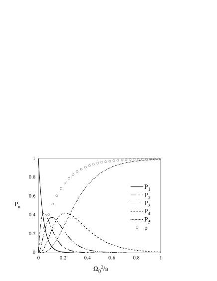
FIG. 3.: The transition probabilities for the $f=2$ multistate Landau-Zener model. The two-state solution is given by $p$, and goes clearly faster to unity with increasing $\Omega_{0}^{2}/a$ than the corresponding five-state probability $P_{5}$.

The Landau-Zener model can also describe the chirped output coupling. Then the atoms are assumed to be stationary, so the time-dependence in $\Delta$ arises from the time-dependent change in $\omega_{\rm rf}$ (chirp), which is typically linear in time. In Ref. [3] the three-state version of the result (19) was successfully used in describing the corresponding experiment in sodium $f=1$ system. However, there the model was introduced only intuitively, and justified merely by a comparison with numerical solutions to Eq. (3). Here we have provided the proof that the $f=1$ solution is exact, and furthermore, derived the exact solution for any $f$. The special case of the three-state Landau-Zener model is also studied in Ref. [12].

Instead of a chirped field one can use resonant pulsed output coupling, which was also demonstrated in Ref. [3]. For any resonant pulse we have $\Delta=0$ and thus the two-state system follows the area theorem [7, 8]:

$$p=\sin^{2}(A/2),\qquad A=2\int_{-\infty}^{\infty}dt\,\Omega(t),$$ (22)

where $A$ is defined as the pulse area, typically $A\propto\Omega_{0}T$ (here $\Omega_{0}$ is the pulse peak amplitude and $T$ is the pulse duration). In the MIT experiment [3] the number of atoms left in the trap oscillated as a function of the area of a resonant square pulse, exactly as Eqs. 19 and (22) predict. However, our model is not limited to resonant pulses only. For off-resonant pulses ($\Delta=const\neq 0$) in two-state systems there are several known analytic solutions, which are reviewed e.g. in Refs. [7, 8].

The purely time-dependent output coupler models described above are valid only if the time scales for the rf-induced interaction and the spatial dynamics of the condensate are very different. In molecular systems one expects interesting effects when the excitation process and internal dynamics of the molecule couple [8]. It might be possible to realize some of the predicted molecular wave packet phenomena using condensates.

In this Letter we have shown that any time-dependent multistate model describing the rf-induced coupling between the different atomic spins states within the same hyperfine manifold can always be solved in terms of the solution of the corresponding two-state model. The fact that these models play a crucial role in time-dependent control of magnetically trapped ultracold atoms adds significantly to the importance of this result, which is also in general quite fascinating.

This research has been supported by the Academy of Finland. K.-A. S. thanks Paul Julienne for enlightening discussions on evaporative cooling.

REFERENCES

- [1] W. Ketterle and N. J. van Druten, Adv. At. Mol. Opt. Phys. 37, 181 (1996).
- [2] M. H. Anderson et al., Science 269, 198 (1995); C. C. Bradley et al., Phys. Rev. Lett. 75, 1687 (1995); K. B. Davis et al., Phys. Rev. Lett. 75, 3969 (1995); M.-O. Mewes et al., Phys. Rev. Lett. 77, 416 (1996).
- [3] M.-O. Mewes et al., Phys. Rev. Lett. 78, 582 (1997).
- [4] M. R. Andrews et al., Science 275, 637 (1997).
- [5] D. E. Pritchard et al., At. Phys. 11, 179 (1989).
- [6] K. B. Davis et al., Phys. Rev. Lett. 74, 5202 (1995).
- [7] B. W. Shore, The Theory of Coherent Atomic Excitation, Vol. 1 (Wiley, New York, 1990).
- [8] B. M. Garraway and K.-A. Suominen, Rep. Prog. Phys. 58, 365 (1995).
- [9] M. E. Rose, Elementary Theory of Angular Momentum (Wiley, New York, 1957); R. N. Zare, Angular Momentum (Wiley, New York, 1988).
- [10] R. J. Cook and B. W. Shore, Phys. Rev. A 20, 539 (1979).
- [11] C. Zener, Proc. R. Soc. Lond. Ser. A 137, 696 (1932); K.-A. Suominen et al., Opt. Commun. 82, 260 (1991); N. V. Vitanov and B. M. Garraway, Phys. Rev. A 53, 4288 (1996).
- [12] C. E. Carroll and F. T. Hioe, J. Phys. B 19, 1151 (1986); J. Phys. B 19, 2061 (1986).