A NUMERICAL STUDY OF ABSORPTION BY MULTILAYERED BIPERIODIC STRUCTURES

Abstract

We study the electromagnetic scattering by multilayered biperiodic aggregates of dielectric layers and gratings of conducting plates. We show that the characteristic lengths of such structures provide a good control of absorption bands. The influence of the physical parameters of the problem (sizes, impedances) is discussed.

I INTRODUCTION

Electromagnetic absorbers and frequency selective surfaces (FFS for short) have recently received an increasing interest. There is a growing need for electromagnetic absorbers, and in particular for lighter, thinner and more highly absorbing materials. Frequency selective surfaces are generally made of planar screens with periodic or biperiodic metallizations. One generally considers two types of FFS: capacitive FFS are transparent at low frequencies; inductive FFS are reflecting ones. Their behavior at the resonance frequency is complementary. Capacitive FFS consist of arrays of metal patches embedded in a dielectric structure, which may be a stratified one. The dielectric structure provides the mechanical support of the FFS. Inductive FFS consist of perforated screens.

Such frequency selective surfaces have been considered by several authors [1, 6, 13] who have proposed various approaches for the numerical resolution of the corresponding scattering problem. Efficient numerical methods are now available for the analysis and design of FFS, as we shall show.

The purpose of this paper is to show that the absorption bands of such structures may be controlled by combining the performances of capacitive FFS and electromagnetic absorbers. To vary the frequency response of a FFS, the standard method consists in varying the geometry of the array elements. We give efficient computational methods for analyzing this kind of structure. The representation of the transmitted and reflected fields is obtained by applying resistive boundary conditions to include a general surface impedance in the problem formulation.

We provide examples of such periodic or biperiodic structures, whose absorption bands can easily be controlled by varying some of the characteristic lengths of the system. More precisely, we consider multilayers made of dielectric stacks and surface gratings with various shapes and sizes. We show that such structures yield absorption bands, and that the location and bandwidth of such bands may be controlled by varying the characteristic sizes of the structure.

This paper is organized as follows. After this introduction, we describe in Section II the details of the diffracting structures we consider, and the model we use to solve numerically the corresponding diffraction problem. Then we develop in section III the numerical resolution method, and discuss a series of examples. Finally, section IV is devoted to the conclusions. More technical aspects concerning the mathematical background and numerical details are discussed in three appendices at the end of this paper.

II MODELLING THE BIPERIODIC STRUCTURES

We consider a system made of dielectric layers and biperiodic gratings of resistive conducting plates, ended by an infinitely conducting plane (or the vacuum), located at a height $z=0$. The structure is globally invariant under the discrete translations of period $(a,b)$ which define the grating, namely translations of the form $x\to x+ma$, $y\to y+nb$, $m,n\in Z\kern-5.0pt{Z}$, in the $xOy$ plane. The structure is illuminated by an incident monochromatic field of the form

$$\overrightarrow{E}^{I}(x,y,z)=\overrightarrow{E}^{I}\,e^{-i(\omega t-\overrightarrow{k}.\overrightarrow{r})}\ .$$

The geometry of the problem is displayed in Fig 1. We shall generically denote by $E^{(j)}$ and $H^{(j)}$ the electric and magnetic fields in the $j$-th layer $z_{j}<z<z_{j+1}$, with electric permittivity $\epsilon_{j}$; we shall also use the superscript $+$ or $-$, according to whether the field propagates in the direction of positive or negative $z$. From now on, the configuration of Fig. 1 will be refered to as configuration I.

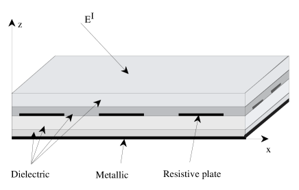
FIG. 1.: Global geometry of the structure: a grating of resistive plates between stacks of dielectric media, upon a perfectly conducting plane. The incident field propagates in the direction of negative $z$.

Alternatively, we shall also consider the same structure, but we remove the infinitely conducting plane at $z=0$. The latter configuration will be called configuration II.

A Floquet Modes

Taking into account the global invariance of the problem, it is natural to introduce the associated Floquet decompositions. Let $\overrightarrow{k}=(k_{x},k_{y},k_{z})$ be the incident wavevector. In a medium of permittivity $\epsilon$, let us set for all integers $m,n$

$$\left\{\begin{array}[]{lll}&\alpha_{0}=k_{x}\sqrt{\epsilon}\ ,&\alpha_{m}=\alpha_{0}+\displaystyle{\frac{2\pi m}{a}}\ ,\\ &\beta_{0}=k_{y}\sqrt{\epsilon}\ ,&\beta_{n}=\beta_{0}+\displaystyle{\frac{2\pi n}{b}}\ ,\\ &t_{mn}=\sqrt{\alpha_{m}^{2}+\beta_{n}^{2}}\ ,&\gamma_{mn}^{2}=k^{2}-t_{mn}^{2}\ ,\end{array}\right.$$ (1)

where $a$ and $b$ are the grating periods. For $m,n$ integers, we introduce the corresponding Floquet modes

$${\cal E}_{mn}^{\pm}(x,y,z)=\frac{1}{\sqrt{ab}}e^{i(\alpha_{m}x+\beta_{n}y\pm\gamma_{mn}z)}\ ,$$ (2)

and the “planar” modes

$$\phi_{mn}(x,y)=\frac{1}{\sqrt{ab}}e^{i(\alpha_{m}x+\beta_{n}y)}\ ,$$ (3)

which form an orthonormal basis of the space of biperiodic functions on the plane, with period $(a,b)$. Then it is well known that such function satisfy Helmholtz’s equation, and that both the electric and the magnetic fields may be decomposed into those Floquet modes (see e.g.  [11]). Therefore, we write in the $j$-th layer

$$\overrightarrow{E}^{(j)}\!\!\!\!(x,\!y,\!z)\! = \!\!\!\sum_{m,n}\!\!\left(\!\!\overrightarrow{e}^{(j)+}_{mn}\!\!{\cal E}_{mn}^{+}(x,\!y,\!z)+\!\!\overrightarrow{e}^{(j)-}_{mn}\!\!{\cal E}_{mn}^{-}(x,y,z)\right)\!,$$ (4)

$$\overrightarrow{H}^{(j)}\!\!\!\!(x,\!y,\!z)\! = \!\!\!\sum_{m,n}\!\!\left(\!\!\overrightarrow{h}^{(j)+}_{mn}\!\!{\cal E}_{mn}^{+}(x,\!y,\!z)+\!\!\overrightarrow{h}^{(j)-}_{mn}\!\!{\cal E}_{mn}^{-}(x,\!y,\!z)\right)\ ,$$ (5)

where $\overrightarrow{e}^{(j)\pm}_{mn}$ and $\overrightarrow{h}^{(j)\pm}_{mn}$ denote the (complex vector) coefficients of the expansion. The sum over $m,n$ runs theoretically from $-\infty$ to $\infty$. In practice it has to be truncated to a finite index $[-M,M]\times[-N,N]$. We now restrict ourselves to the tangential electric and magnetic fields. We directly obtain from Maxwell’s equations that the following matrix relations hold

$$\overrightarrow{h}_{mn}^{(j)\pm}=\mp{\bf K}_{mn}^{(j)}{\bf X}\overrightarrow{e}_{mn}^{(j)\pm}\ .$$ (6)

Here we have introduced the following $2\times 2$ matrices:

$${\bf K}_{mn}^{(j)}\!=\!\frac{1}{\omega\mu\gamma_{mn}}\!\left(\!\begin{array}[]{cc}k^{2}-\alpha_{m}^{2}&-\alpha_{m}\beta_{n}\\ -\alpha_{m}\beta_{n}&k^{2}-\beta_{n}^{2}\end{array}\!\right)\ ,\ {\bf X}\!=\!\left(\!\begin{array}[]{cc}0&1\\ -1&0\end{array}\!\right)\ .$$ (7)

In the following we set $\xi_{mn}=\frac{1}{\omega\mu\gamma_{mn}}$.

Alternatively, we shall also make use of the expansions with respect to the planar modes $\phi_{mn}(x,y)$ in (3), which leads to the coupled waves, defined by

$$\overrightarrow{E}^{(j)\pm}_{mn}(z) = \overrightarrow{e}^{(j)\pm}_{mn}e^{\pm i\gamma_{mn}z}\ ,$$ (8)

$$\overrightarrow{H}^{(j)\pm}_{mn}(z) = \overrightarrow{h}^{(j)\pm}_{mn}e^{\pm i\gamma_{mn}z}\ .$$ (9)

The propagation of such modes within the corresponding layer is diagonal, and we have in particular

$$\overrightarrow{E}^{(j)\pm}_{mn}(z_{j+1})=\exp\{\pm i\gamma_{mn}(z_{j+1}-z_{j})\}\overrightarrow{E}^{(j)\pm}_{mn}(z_{j})\ .$$ (10)

Matching boundary conditions at a dielectric-dielectric interface is an easy task, since Floquet modes with different indices are not coupled. Given one such interface between two dielectric media labeled by $j$,$j+1$, at a height $z=z_{j}$, and equating the tangential components of the electric and magnetic fields, we obtain:

$$\left(\!\!\begin{array}[]{c}\overrightarrow{E}_{mn}^{(j)+}\\ \overrightarrow{E}_{mn}^{(j)-}\end{array}\!\!\right)\!=\!C_{mn}^{(j)}\!\!\left(\!\!\begin{array}[]{c}\overrightarrow{E}_{mn}^{(j+1)+}\\ \overrightarrow{E}_{mn}^{(j+1)-}\end{array}\!\!\right)\!=\!\left(\!\!\begin{array}[]{cc}{\bf c}&{\bf c}^{\prime}\\ {\bf c}^{\prime}&{\bf c}\end{array}\!\!\right)\!\!\left(\!\!\begin{array}[]{c}\overrightarrow{E}_{mn}^{(j+1)+}\\ \overrightarrow{E}_{mn}^{(j+1)-}\end{array}\!\!\right)\ ,$$ (11)

where for the sake of simplicity we have suppressed the explicit dependence on the height $z=z_{j}$. The matrix elements (which are themselves $2\times 2$ matrices) ${\bf c},{\bf c}^{\prime}$ are given by

$${\bf c} ={\bf c}^{(j)}_{mn} =\frac{1}{2}({\bf X})^{-1}\left(1+({\bf K}_{mn}^{(j)})^{-1}{\bf K}_{mn}^{(j+1)}\right){\bf X}\ ,$$ (12)

$${\bf c}^{\prime} ={\bf c}^{\prime(j)}_{mn} =\frac{1}{2}({\bf X})^{-1}\left(1-({\bf K}_{mn}^{(j)})^{-1}{\bf K}_{mn}^{(j+1)}\right){\bf X}\ .$$ (13)

Alternatively, we shall make use of the following $R$-matrices, which read

$$\left(\!\!\begin{array}[]{c}\overrightarrow{E}_{mn}^{(j+1)+}\\ \overrightarrow{E}_{mn}^{(j)-}\end{array}\!\!\right)\!=\!R_{mn}^{(j)}\!\left(\!\!\begin{array}[]{c}\overrightarrow{E}_{mn}^{(j)+}\\ \overrightarrow{E}_{mn}^{(j+1)-}\end{array}\!\!\!\right)\!=\!\left(\!\!\begin{array}[]{cc}{\bf t}^{++}&{\bf r}^{-+}\\ {\bf r}^{+-}&{\bf t}^{--}\end{array}\!\!\right)\!\!\left(\!\!\begin{array}[]{c}\overrightarrow{E}_{mn}^{(j)+}\\ \overrightarrow{E}_{mn}^{(j+1)-}\end{array}\!\!\!\right)\ ,$$ (14)

and the connection between the two formulations is given by [4]

$$R_{mn}^{j}=\left(\begin{array}[]{cc}{\bf c}^{-1}&-{\bf c}^{-1}{\bf c}^{\prime}\\ {\bf c}^{\prime}{\bf c}^{-1}&{\bf c}-{\bf c}^{\prime}{\bf c}^{-1}{\bf c}^{\prime}\end{array}\right)\ .$$ (15)

B Surface Elements and Boundary Conditions on the Conducting Plates

Let us now describe the surface currents living on the conducting plates. We may expand such currents into Floquet modes

$${\overrightarrow{\cal J}}(x,y)=\sum_{m,n}{\overrightarrow{\cal J}}_{mn}\phi_{mn}(x,y)\ ,$$ (16)

and impose the boundary conditions.

FIG. 2.: The grating of conducting plates, in the particular case of rectangular plates.

Several approaches have been proposed for imposing boundary conditions. Among these, the integral formulations (e.g. Galerkin methods) are generally considered the most stable. To implement the Galerkin method, we need to introduce a family of functions defined on the plates. Let $\overrightarrow{\psi}_{pq}(x,y)$ be such a family. If $z_{P}$ denotes the height of the interface supporting the conducting plates, we then write, at a height $z=z_{P}$

$${\overrightarrow{\cal J}}(x,y)=\sum_{p,q}j_{pq}\overrightarrow{\psi}_{pq}(x,y)\ .$$ (17)

The boundary conditions rely on three sets of equations. First, the continuity of the tangential electric fields at all interfaces

$$\overrightarrow{E}^{(j+1)}(x,y,z_{j})=\overrightarrow{E}^{(j)}(x,y,z_{j})\ ,$$ (18)

allows one to connect the global electric fields on each side of the interface. Second, the discontinuity condition for the tangential magnetic fields:

$$\overrightarrow{H}^{(j+1)}(x,y,z_{j})-\overrightarrow{H}^{(j)}(x,y,z_{j})={\bf X}{\overrightarrow{\cal J}}(x,y,z_{j})\ ,$$ (19)

explicitely

$${\bf K}^{j}{\bf X}\!\!\left(\!\!\overrightarrow{E}^{(j)+}_{mn}\!\!\!\!-\!\overrightarrow{E}^{(j)-}_{mn}\!\!\right)\!\!-\!{\bf K}^{j+1}{\bf X}\!\!\left(\!\!\overrightarrow{E}^{(j+1)+}_{mn}\!\!\!\!\!-\!\overrightarrow{E}^{(j+1)-}_{mn}\!\!\right)\!=\!{\bf X}{\overrightarrow{\cal J}}_{mn}\ .$$ (20)

Finally, the impedance boundary conditions, which read at a height $z=z_{P}$:

$$\overrightarrow{E}^{(P+1)}(x,y,z_{P})=\overrightarrow{E}^{(P)}(x,y,z_{P})=Z{\overrightarrow{\cal J}}(x,y,z_{P})\ ,$$ (21)

(where ${\overrightarrow{\cal J}}$ vanishes outside the conducting plates) require a special treatment. It has been observed by several authors that such conditions cannot be imposed pointwise, because this leads to unstable systems. Several alternatives have been proposed and tested (see for example  [6]). The most stable solutions rely on the use of integral formulations, obtained by considering either line integrals of the above equation, or a Galerkin formulation. We limit ourselves to the latter, which leads to a finite number of integral equations, obtained by testing Eq. (21) against suitably chosen basis functions $\psi_{pq}(x,y)$ (see Appendix A for some possible choices).

C The Coupled System

Let us start with the case of configuration I. Taking into account the above remarks, we are led to the following formulation. We denote by $\overrightarrow{E}^{I}$ and $\overrightarrow{E}^{R}$ the incident and reflected electric fields respectively, and we recall that we have denoted by $P$ the index of the interface containing the plates. In order to avoid as much as possible numerical problems, we limit ourselves to a formulation involving the so-called $R$-matrix propagation formalism [4, 5] (see Appendix B for a short account of the method).

Using the $R$-matrix propagation scheme, we can obtain $R$ matrices for the stacks below and above $z=z_{P}$. For example, we obtain a relation of the form

$$\left(\begin{array}[]{c}\overrightarrow{E}^{R}_{mn}\\ \overrightarrow{E}^{(P+1)-}_{mn}\end{array}\right)=\left(\begin{array}[]{cc}{\bf T}^{++}&{\bf R}^{-+}\\ {\bf R}^{+-}&{\bf T}^{--}\end{array}\right)\left(\begin{array}[]{c}\overrightarrow{E}^{(P+1)+}_{mn}\\ \overrightarrow{E}^{I}_{mn}\end{array}\right)\ ,$$ (22)

where the $2\times 2$ matrices ${\bf T}$ and ${\bf R}$ are the stack equivalent transmission and reflection matrices respectively. Similarly, the $R$-matrix algorithm below the grating of plates yields a matrix relation of the form

$$\left(\begin{array}[]{c}\overrightarrow{E}^{(P)+}_{mn}\\ \overrightarrow{E}^{(0)-}_{mn}\end{array}\right)=\left(\begin{array}[]{cc}{\bf T}^{\prime++}&{\bf R}^{\prime-+}\\ {\bf R}^{\prime+-}&{\bf T}^{\prime--}\end{array}\right)\left(\begin{array}[]{c}-\overrightarrow{E}^{(0)-}_{mn}\\ \overrightarrow{E}^{(P)-}_{mn}\end{array}\right)\ ,$$ (23)

which implies

$$\overrightarrow{E}^{(P)+}_{mn} = \left({\bf R}^{\prime-+}-{\bf T}^{\prime++}(1-{\bf T}^{\prime--})^{-1}{\bf R}^{\prime+-}\right)\overrightarrow{E}^{(P)-}_{mn}$$ (24)

$$= {\cal N}^{-1}\overrightarrow{E}^{(P)-}_{mn}\ .$$ (25)

The remarkable point with such a formulation is that it only involves small matrices, since modes with different indices $m,n$ are not coupled. The only place where coupling between Floquet modes occurs is at a height $z=z_{P}$.

The case of configuration II requires only minor modifications. Eq. (22) is still valid. For the stack below the grating of conducting plates, we have to replace Eq. (23) with

$$\left(\begin{array}[]{c}\overrightarrow{E}^{(P)+}_{mn}\\ \overrightarrow{E}^{T}_{mn}\end{array}\right)=\left(\begin{array}[]{cc}{\bf T}^{\prime++}&{\bf R}^{\prime-+}\\ {\bf R}^{\prime+-}&{\bf T}^{\prime--}\end{array}\right)\left(\begin{array}[]{c}0\\ \overrightarrow{E}^{(P)-}_{mn}\end{array}\right)\ ,$$ (26)

where $\overrightarrow{E}^{T}_{mn}$ are the Floquet coefficients of the transmitted field. Therefore, Eq. (25) is to be replaced with

$$\overrightarrow{E}^{(P)+}_{mn}={\bf R}^{\prime+-}\overrightarrow{E}^{(P)-}_{mn}={\cal N}^{-1}\overrightarrow{E}^{(P)-}_{mn}\ .$$ (27)

The rest of the formalism is unchanged.

III RESOLUTION AND NUMERICAL RESULTS

A Resolution of the Coupled System

We now consider the practical resolution of the system we have obtained above. We consider approximations of the fields with $(2N+1)(2M+1)$ Floquet modes $\overrightarrow{E}_{mn},m=-M,\dots M,n=-N,\dots N$, and approximations of the currents with $PQ$ surface elements $\overrightarrow{\psi}_{pq}$. The boundary conditions lead to three systems of equations involving the three sets of unknowns: $\overrightarrow{E}^{(P)+}_{mn}$, $\overrightarrow{E}^{(P+1)+}_{mn}$ and ${\overrightarrow{\cal J}}_{mn}$. Eliminating $\overrightarrow{E}^{(P)+}_{mn}$, we first obtain

$$\overrightarrow{E}^{(P)+}_{mn}\!\!\!\!=\left(1+{\cal N}\right)^{-1}\!\left(\!\left(1+{\bf R}^{+-}_{mn}\right)\overrightarrow{E}^{(P+1)+}_{mn}\!\!\!\!\!\!+{\bf T}^{--}_{mn}\overrightarrow{E}^{I}_{mn}\!\right)\ .$$ (28)

Inserting this result into (19), we get

$$\overrightarrow{E}^{(P+1)+}_{mn}={\bf A}_{mn}^{-1}\left(X{\overrightarrow{\cal J}}_{mn}+{\bf B}_{mn}\overrightarrow{E}^{I}_{mn}\right)\ ,$$ (29)

where we have set

$${\bf A}_{mn}\! = \!\!{\bf K}_{mn}^{(p+1)}\!{\bf X}\left(\!{\bf R}_{mn}^{+-}-1\right)$$ (31)

$$-\!{\bf K}_{mn}^{(p)}\!{\bf X}\left({\cal N}\!-1\right)\left({\cal N}\!+1\right)^{-1}\!\left({\bf R}_{mn}^{+-}\!+1\!\right)\!\ ,$$

$${\bf B}_{mn}\! = \!\!\left({\bf K}_{mn}^{(p)}\!{\bf X}\left({\cal N}\!-1\right)\!\left({\cal N}\!+1\right)^{-1}-\!\!{\bf K}_{mn}^{(p+1)}\!{\bf X}\right)\!{\bf T}_{mn}^{--}\ .$$ (32)

Eventually, we are led to a system of the form

$${\bf U}_{mn}\overrightarrow{E}^{I}_{mn}={\bf V}_{mn}{\overrightarrow{\cal J}}_{mn}\ ,$$ (33)

where the $2\times 2$ matrices ${\bf U}_{mn}$ and ${\bf V}_{mn}$ are defined by:

$${\bf U}_{mn} = {\bf T}_{mn}^{--}+\left(1+{\bf R}_{mn}^{+-}\right){\bf A}_{mn}^{-1}{\bf B}_{mn}\ ,$$ (34)

$${\bf V}_{mn} = Z-\left(1+{\bf R}_{mn}^{+-}\right){\bf A}_{mn}^{-1}{\bf X}\ .$$ (35)

The system (33) is to be solved numerically, using a Galerkin procedure. Let $\overrightarrow{\psi}_{pq}(x,y)$ be a basis of functions defined on the plate, with appropriate boundary conditions. Using the expansion (17), we get

$${\overrightarrow{\cal J}}_{mn}=\sum_{p,q}j_{pq}\overrightarrow{\psi}_{pq;mn}\ ,$$ (36)

where

$$\overrightarrow{\psi}_{pq;mn}=\langle\overrightarrow{\psi}_{pq},\phi_{mn}\rangle=\int\overrightarrow{\psi}_{pq}(x,y)\phi_{mn}^{*}(x,y)dxdy\ ,$$ (37)

and where the star “$*$” denotes complex conjugation. Taking the scalar products of equations (33) with the basis functions $\overrightarrow{\psi}_{pq}(x,y)$, we obtain a system of the form

$${\cal U}_{pq}=\sum_{p^{\prime},q^{\prime}}{\cal V}_{pq;p^{\prime}q^{\prime}}j_{p^{\prime}q^{\prime}}\ ,$$ (38)

where ${\cal U}$ is a vector of length $PQ$ and ${\cal V}$ is a $PQ\times PQ$ matrix given by

$${\cal U}_{pq} = \sum_{m,n}\left({\bf U}_{mn}\overrightarrow{E}^{I}_{mn}\right)\cdot\overrightarrow{\psi}_{pq;mn}^{*}\ ,$$ (39)

$${\cal V}_{pq;p^{\prime}q^{\prime}} = \sum_{m,n}\left({\bf V}_{mn}\overrightarrow{\psi}_{p^{\prime}q^{\prime};mn}\right)\cdot\overrightarrow{\psi}_{pq;mn}^{*}\ .$$ (40)

Eq. (38) is solved numerically (more details are given in Appendix C). Once the current ${\overrightarrow{\cal J}}$ is known, one recovers directly the fields $\overrightarrow{E}^{(P+1)+}_{mn}$ using Eq. (29) and then the reflected field $\overrightarrow{E}^{R}$, from Eq. (22).

B Numerical Results

Our main goal is to exhibit absorption bands, and to analyze the influence of some specific parameters on the location of the maximal absorption. More precisely, we focus on the influence of the resistive impedance $Z$ and the ratio size of resistive plates/period. In addition, we show that the location of the absorption band essentially does not depend on the incidence angle. We work with a TM polarization for the incident field (in fact the results are weakly dependent on the polarization).

We consider a series of configurations, in which we vary individually these parameters, in the frequency domain $1GHz-10GHz$. In all the figures, we plot the reflectivity (i.e. the ratio of reflected flux by incident flux) as a function of the incident frequency, and in the case of configuration II we also plot the transmittivity (i.e. the ratio of transmitted flux by incident flux).

We start with the case of square resistive plates of sidelength $a^{\prime}$, with variable impedance. The period of the grating is set to $a=10mm$ in both the $x$ and $y$ directions. The grating is supported by a dielectric stack of height $z=4mm$ and complex refractive index $\epsilon=10+2i$, itself supported by an infinitely conducting plane (a simple case of configuration I). Since the resistive plates are in that case square plates, we use Fourier-type decompositions as described in Appendix A 1 for the decomposition of the surface current. The numerical results displayed below have been obtained using $17\times 17$ Floquet modes and the same number of Galerkin modes.

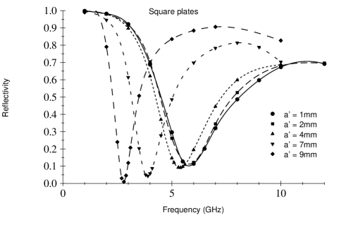
FIG. 3.: Square plates in configuration I. Reflectivity as a function of the incident frequency, for various values of the plate’s size: $a^{\prime}=1,2,4,7,9mm$. The period $a$ is kept fixed to $a=10mm$. $\theta=0$ and $Z=0$.

We show in Figure 3 the reflectivity as a function of the incident frequency, for several values of the ratio $a^{\prime}/a$. The computed values are indicated with symbols, and intermediate values have been obtained using cubic spline interpolation. In all cases, a significant absorption band is observed. In addition, the critical frequency (i.e. the frequency at which reflectivity attains its minimum) decreases as the ratio $a^{\prime}/a$ increases, and the width of the absorption band narrows.

In the considered case, the plates are perfectly conducting. We nevertheless observe a strong absorption in a specific frequency range. Such a phenomenon is generally coupled with the excitation of a leaky surface wave. The surface wave may be given an interpretation in terms of complex poles or zeroes of a scattering matrix (see [8] for details on the scattering matrix, and [9] for an analysis of the role of zeroes and poles). The poles of the scattering matrix give the propagation constant of the leaky waves, which propagate along the surface of the biperiodic grating. The leaky wave is evanescent, as its energy decreases in the direction normal to the surface of the structure. The imaginary part of the pole gives the damping of the wave. The excitation of a leaky wave is a resonance phenomenon at a particular frequency. Figure 3 shows a spectacular phenomenon. A highly reflecting capacitive grating (with an important ratio $a^{\prime}/a$) can absorb an incident plane wave in totality. Thanks to this absorption by a leaky surface wave propagating along the grating, we can control the absorption band of a classical Dahlenbach absorber layer which consists of a thick homogeneous lossy layer backed by a metallic plate. When the ratio $a^{\prime}/a$ tends to zero we have checked that the minimum of reflectivity is obtained for the same frequency as in Figure 3. To adjust the absorption band of the absorber, we can deposit a biperiodic capacitive reflecting grating on the Dahlenbach layer. By doing so, we combine the properties of the biperiodic grating with those of the lossy layer. Notice in particular that it is possible to decrease the thickness of the layer by adding such a biperiodic structure, to obtain the critical absorption frequency of the initial Dahlenbach structure.

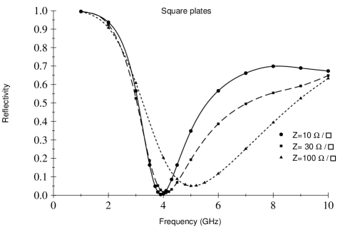
FIG. 4.: Square plates in configuration I. Reflectivity as a function of the incident frequency, for various values of the plate’s impedance: $Z=10,30,100\Omega/\Box$. The period $a$ and the plate’s size $a^{\prime}$ are kept fixed $a=10mm$ and $a^{\prime}=7mm$. $\theta=0$.

We show in Figure 4 the reflectivity as a function of the frequency of the incident beam, for several values of the impedance $Z$. The configuration corresponds to the case of Fig. 3 with $a^{\prime}=7mm$, and a significant minimum in the reflectivity is observed for a certain value of the frequency. This critical value is seen to be an increasing function of the impedance of the conducting plates.

In Figure 4, the patches of the grating are not perfectly conducting any more. In that case, the absorption frequency and the bandwidth increase with the resistivity of the patches. To obtain a required absorption band, it is therefore possible to combine the effects of the geometry (here the ratio $a^{\prime}/a$) and the effect of the conductivity. This provides extra flexibility to the filter design.

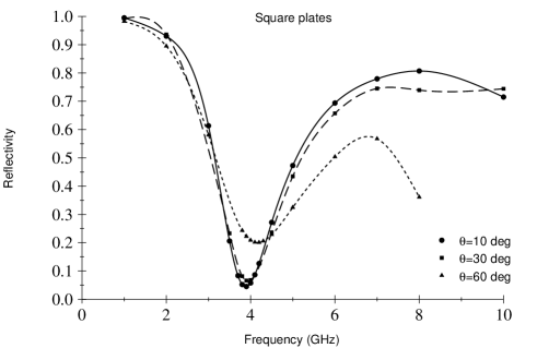
FIG. 5.: Square plates in configuration I. Reflectivity as a function of the incident frequency, for various values of incidence angle: $\theta=10,30,60\ deg$. The period $a$ and the plate’s size $a^{\prime}$ are kept fixed $a=10mm$ and $a^{\prime}=7mm$. $Z=0$.

We show in Figure 5 the reflectivity as a function of the frequency of the incident beam, for several values of the incidence angle $\theta$, for the same configuration as before, i.e. a configuration exhibiting a well defined absorption band. These results (and other tests of intermediate incidence angles, are not reproduced here to simplify the plot) show that the critical frequency value depends very weakly on the incidence angle (at least for angles smaller than 45 deg).

The same computations have been performed with resistive plates of various shapes. We display here the results obtained when the square resistive plates in Fig. 3 are replaced with cross-shaped ones, of the same size. By this we mean that the crosses lie within a square of the sidelength $a^{\prime}$, and are made of five identical squares of sidelength $a^{\prime}/3$. For this case, we used the surface elements described in Appendix A 2, and as before we take $17\times 17$ Floquet modes, and the same number of Galerkin modes.

The numerical results, displayed in Figures 6 and 7 show a similar behavior to the previous case: a well defined absorption band is clearly seen, and the critical frequency again depends on the ratio $a^{\prime}/a$ and on the impedance $Z$. Again, the location of the absorption band depends only weakly on the incidence angle (the numerical results, not given here, are very similar to those displayed in Fig. 5). The only significant difference which may be observed is a broadening of the absorption band in the case of cross-shaped plates, and a second minimum occurs for large $a^{\prime}$.

FIG. 6.: Cross-shaped plates in configuration I. Reflectivity as a function of the incident frequency, for various values of the plate’s size: $a^{\prime}=1,2,4,7,9mm$. The period $a$ is kept fixed to $a=10mm$. $\theta=0$ and $Z=0$.

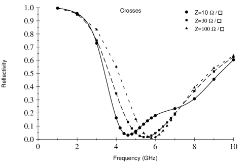
FIG. 7.: Cross-shaped plates in configuration I. Reflectivity as a function of the incident frequency, for various values of the plate’s impedance: $Z=10,30,100\Omega/\Box$. The period $a$ and the plate’s size $a^{\prime}$ are kept fixed $a=10mm$ and $a^{\prime}=7mm$. $\theta=0$.

Similar computations have been made with configuration II. We display in Fig. 8 (reflexion) and Fig. 9 (transmission) the results obtained with systems identical to those considered in Figures 3-5. We observe that in such a configuration, the reflexion is small and almost constant above $5Ghz$, it increases slightly with $a^{\prime}$. The transmittivity shows maximums at frequencies corresponding to the minimums in configuration I.

These two figures show the importance of the conducting plane at $z=0$. The well-defined absorption band appears only in that case. The excitation of the leaky wave and the corresponding absorption occurs only for structures ended by a conducting plane.

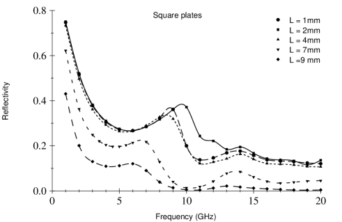
FIG. 8.: Reflexion for square plates in configuration II. Reflectivity as a function of the incident frequency, for various values of the plate’s size: $a^{\prime}=1,2,4,7,9mm$. The period $a$ is kept fixed to $a=10mm$. $\theta=0$ and $Z=0$.

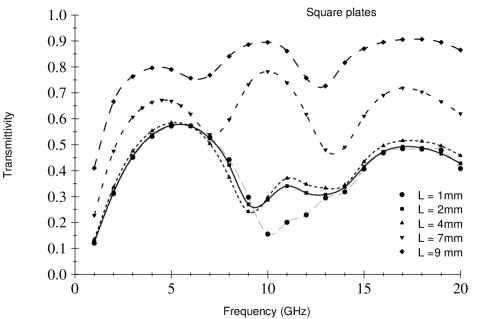
FIG. 9.: Transmission for square plates in configuration II. Reflectivity as a function of the incident frequency, for various values of the plate’s size: $a^{\prime}=1,2,4,7,9mm$. The period $a$ is kept fixed to $a=10mm$. $\theta=0$ and $Z=0$.

Next, we consider a second system (in configuration I), in which the resistive plates are located upon a double layer of dielectrics. The first dielectric (upon which the plates are located) has electric permittivity $\epsilon=5$, and the second layer has electric permittivity $\epsilon=15+i18\sigma/\nu$ with a frequency dependent imaginary part. Here the constant $\sigma$ is set to $\sigma=10s/m$, and the frequency $\nu$ is expressed in $GHz$.

The results are displayed in Figures 10 and 11. As before, an absorption band is clearly seen on Figure 10, when $a^{\prime}$ is above 4mm, whose critical frequency and bandwidth decrease as the sidelength of the plates increases. In addition, for small plates, the reflectivity has a constant behavior close to zero above $8GHz$. Figure 11 shows that in such a configuration, the critical frequency depends weakly on the value of the impedance, but the bandwidth is an increasing function of the impedance.

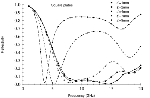
FIG. 10.: Reflexion for square plates in configuration I. Reflectivity as a function of the incident frequency, for various values of the plate’s size: $a^{\prime}=1,2,4,7,9mm$. The period $a$ is kept fixed to $a=10mm$. $\theta=0$ and $Z=0$.

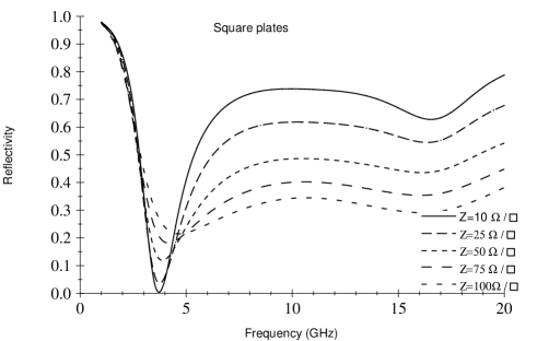
FIG. 11.: Reflexion for square plates in configuration I. Reflectivity as a function of the incident frequency, for various values of the resistive impedance $Z$: $Z=10,25,50,75,100\Omega/\Box$. The period $a$ is kept fixed to $a=10mm$. $a^{\prime}=7mm$ and $\theta=0$.

IV CONCLUSIONS AND PERSPECTIVES

We have studied and described a series of configurations involving dielectric stacks and arrays or resistive plates which produce well-defined absorption bands, with controllable absorption frequency. The critical frequency has been shown to be strongly influenced by the ratio period/plate-size, which therefore provides a good control parameter. The impedance of the resistive plates has been shown to allow the control of the critical frequency.

Our approach is based on a Floquet (or Rayleigh) development of the electromagnetic fields within the different layers of the structure, and a Galerkin approximation of the surface currents. Multilayers more complex than the ones we considered here may be described by the formalism of this paper as well.

In light of the numerical experiments we have performed, it is possible to combine the different parameters (namely the ratio $a^{\prime}/a$, the geometry of the patches and the conductivity of the patch material) to obtain optimized absorbing structures from a quite standard biperiodic grating. The use of absorption by a leaky surface wave can improve a classical Dahlenbach structure.

A THE SURFACE ELEMENTS

Depending on the geometry of the conducting plates, several different bases of surface elements may be used. In all cases, the finite number of basis functions we are forced to consider limits the precision of the approximation of the current.

1 Rectangular Plates

To start with, we consider the case of rectangular plates, as shown in Fig. 2 above. In such cases, the best choice for surface elements is provided by a Fourier basis: we set

$$\vec{\psi}^{TE}_{pq}(x,y) = ~{}~{}{p\pi\over a^{\prime}}\sin{{p\pi\over a^{\prime}}[x+{\textstyle\frac{1}{2}}a^{\prime}]}\cos{{q\pi\over b^{\prime}}[y+{\textstyle\frac{1}{2}}b^{\prime}]}\vec{e}_{x}$$ (A2)

$$+{q\pi\over b^{\prime}}\cos{{p\pi\over a^{\prime}}[x+{\textstyle\frac{1}{2}}a^{\prime}]}\sin{{q\pi\over b^{\prime}}[y+{\textstyle\frac{1}{2}}b^{\prime}]}\vec{e}_{y}\ ,$$

$$\vec{\psi}^{TM}_{pq}(x,y) = ~{}~{}{q\pi\over b^{\prime}}\sin{{p\pi\over a^{\prime}}[x+{\textstyle\frac{1}{2}}a^{\prime}]}\cos{{q\pi\over b^{\prime}}[y+{\textstyle\frac{1}{2}}b^{\prime}]}\vec{e}_{x}$$ (A4)

$$-{p\pi\over a^{\prime}}\cos{{p\pi\over a^{\prime}}[x+{\textstyle\frac{1}{2}}a^{\prime}]}\sin{{q\pi\over b^{\prime}}[y+{\textstyle\frac{1}{2}}b^{\prime}]}\vec{e}_{y}\ .$$

Therefore, the Floquet modes of the surface current may be written as

$${\overrightarrow{\cal J}}_{mn}=\sum_{p=0}^{P-1}\sum_{q=0}^{Q-1}\left(j_{pq}^{TM}\overrightarrow{\psi}^{TM}_{pq,mn}+j_{pq}^{TE}\overrightarrow{\psi}^{TE}_{pq,mn}\right)\ ,$$ (A5)

and the scalar products

$$\overrightarrow{\psi}^{TE}_{pq,mn} = {\langle}\vec{\psi}^{TE}_{pq},\phi_{mn}{\rangle}\ ,$$ (A6)

$$\overrightarrow{\psi}^{TM}_{pq,mn} = {\langle}\vec{\psi}^{TM}_{pq},\phi_{mn}{\rangle}\ ,$$ (A7)

may be computed analytically.

For other special geometries, such as disks or elongated disks, it is possible to design appropriate basis functions to describe the current density on the resistive plates (in the case of disks, such basis functions are linear combinations of Bessel functions). However, it is also desirable to have basis functions which can describe arbitrary geometries. This is the purpose of the surface elements described in the next subsection.

2 Arbitrary Plates

For conducting plates with arbitrary geometry, we are forced to use “all purpose” basis functions, which we shall call surface elements. Such basis functions have been considered by several authors under the name of rooftop functions. It follows from the analysis in [6] that rooftop functions often provide faster and better conditioned numerical schemes than classical alternatives (the so-called surface-patch and triangular patch functions). The first step for the construction of such surface elements is a discretization of the plate. For the sake of simplicity, we restrict to a uniform square discretization, with period $\tau$. Consider the characteristic function

$$\chi(x)=\left\{\begin{array}[]{ll}1&\hbox{ if }0\leq x\leq\tau\\ 0&\hbox{ elsewhere}\end{array}\right.$$ (A8)

and the Schauder function

$$\Lambda(x)=\left\{\begin{array}[]{ll}1+\frac{x}{\tau}&\hbox{ if }-\tau\leq x\leq 0\\ 1-\frac{x}{\tau}&\hbox{ if }0\leq x\leq\tau\\ 0&\hbox{ elsewhere}\end{array}\right.$$ (A9)

Then set

$$\psi^{x}_{pq}(x,y)=\chi(x-p\tau)\Lambda(y-q\tau)\ ,$$ (A10)

$$\psi^{y}_{pq}(x,y)=\Lambda(x-p\tau)\chi(y-q\tau)\ ,$$ (A11)

and finally

$$\overrightarrow{\psi}_{pq}(x,y)=\psi_{pq}^{x}\vec{e}_{x}+\psi_{pq}^{y}\vec{e}_{y}\ .$$ (A12)

The surface elements we consider will be those functions $\psi^{x}_{pq}(x,y)$ and $\psi^{y}_{pq}(x,y)$ such that their support is completely included in the support of the plate. Clearly, the smaller $\tau$ the better is the approximation of the current, but the higher the complexity of the numerical problem.

B $R$-MATRIX PROPAGATION

We describe briefly the $R$-matrix propagation scheme as we used it in our simulations. Clearly, the simplest approach amounts to consider the direct product of the $C$ matrices given in Eq. (11), which yields directly a $C$ matrix for the whole structure. As stressed by various authors, such a scheme turns out to become rapidly unstable as the depth of the structure grows.

FIG. 12.: Illustration of the $R$-matrix propagation algorithm: the role of an interface $R$-matrix.

Let us consider a multilayered medium with interfaces at heights $z_{p},\dots,z_{F}$, and assume that we are given an interface $R$-matrix of the form given in Eq. (14). Then, one easily verifies that

$$\left(\begin{array}[]{c}\overrightarrow{E}^{(j+1)+}(z_{j})\\ \overrightarrow{E}^{(j)-}(z_{j-1})\end{array}\right)=\left(\begin{array}[]{cc}{\tilde{\bf t}}^{++}&{\tilde{\bf r}}^{-+}\\ {\tilde{\bf r}}^{-+}&{\tilde{\bf t}}^{++}\end{array}\right)\left(\begin{array}[]{c}\overrightarrow{E}^{(j)+}(z_{j-1})\\ \overrightarrow{E}^{(j+1)-}(z_{j})\end{array}\right)\ ,$$ (B1)

where we have set

$$\left\{\begin{array}[]{l}{\tilde{\bf t}}^{++}={\bf t}^{++}L_{j}\,;\ {\tilde{\bf t}}^{--}={\bf t}^{--}L_{j}\,;\\ {\tilde{\bf r}}^{++}={\bf r}^{+-}L_{j}^{2}\,;\ {\tilde{\bf r}}^{-+}={\bf r}^{-+}\ ,\\ L_{j}=\exp\{i\gamma_{mn}(z_{j+1}-z_{j})\}\ .\end{array}\right.$$ (B2)

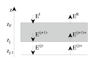
FIG. 13.: Illustration of the $R$-matrix propagation algorithm: the stack $R$-matrix.

Suppose now that we are given a stack $R$-matrix for the stack $[j+1,F]$:

$$\left(\begin{array}[]{c}\overrightarrow{E}^{R}\\ \overrightarrow{E}^{(j)-}\end{array}\right)=\left(\begin{array}[]{cc}{\bf T}^{++}&{\bf R}^{-+}\\ {\bf R}^{-+}&{\bf T}^{++}\end{array}\right)\left(\begin{array}[]{c}\overrightarrow{E}^{(j)+}\\ \overrightarrow{E}^{I}\end{array}\right)\ ,$$ (B3)

where we set by default $\overrightarrow{E}^{(j)\pm}=\overrightarrow{E}^{(j)\pm}(z_{j-1})$ for the sake of simplicity. From Eqs. (B1) and (B3), little algebra gives the expression of the coefficients of the stack matrix for the stack $[j+1,F]$:

$$\overrightarrow{E}^{R}(z_{F}) = {\bf T}^{++}(1\!\!-{\bf R}^{+-}{\tilde{\bf r}}^{-+})^{-1}{\tilde{\bf t}}^{++}\overrightarrow{E}^{(j)+}\!\!\!\!\!(z_{j-1})$$ (B4)

$$+ \left({\bf R}^{-+}\!\!+{\bf T}^{++}(1\!\!-{\bf R}^{+-}{\tilde{\bf r}}^{-+})^{-1}{\tilde{\bf r}}^{-+}{\bf T}^{--}\right)\overrightarrow{E}^{I}(z_{F})\ ,$$ (B5)

$$\overrightarrow{E}^{(j)-}\!\!\!\!\!(z_{j-1}) = \left({\tilde{\bf r}}^{+-}\!\!+\!{\tilde{\bf t}}^{--}(1\!\!-{\bf R}^{+-}{\tilde{\bf r}}^{-+})^{-1}{\tilde{\bf r}}^{-+}{\tilde{\bf t}}^{++}\right)\overrightarrow{E}^{(j)+}\!\!\!\!\!(z_{j-1})$$ (B6)

$$+ {\tilde{\bf t}}^{--}(1\!\!-{\bf R}^{+-}{\tilde{\bf r}}^{-+})^{-1}{\bf T}^{--}\overrightarrow{E}^{I}(z_{F})\ .$$ (B7)

The above equations provide a simple iterative algorithm for computing the global $R$-matrix for the stacks $[z_{P},z_{F}]$ and $[z_{0},z_{P}]$. This algorithm is known as the $R$-matrix propagation algorithm, and has been analyzed by various authors. We refer to [4, 5, 7, 10] for more details.

C NUMERICAL ASPECTS

We give here more details on the numerical methods used to solve the complete problem. As stressed before, most of the matrices used in the scheme are $2\times 2$ matrices, which are easy to handle. In addition, the use of $R$-matrix propagation algorithm prevents us from developing numerical instabilities when computing products of such matrices.

The main part of CPU is used for solving Eq. (38). Several methods have been tested for that problem (which has also been studied by various authors). The numerical results presented here have been obtained by using an inversion method based on $LU$-decomposition, with left and rigth equilibrations of the matrix. A fortran implementation of such a method is available in the LAPACK library (see [3]). Alternative methods may be found in the literature, such as (complex) biconjugate gradient methods or FFT-based methods.

REFERENCES

• [1] C.C. Chen (1979): Transmission through a Conducting Screen Perforated Periodically with Apertures, IEEE Trans. on Microwave Theory and Techniques 9 pp. 627-632.
• [2] J. Dongarra et al (1995):Templates for Iterative Resolution of Linear Systems, SIAM Editions.
• [3] E. Anderson et al. (1992): LAPACK’s user guide, SIAM, Philadelphia.
• [4] L. Li (1993): Multilayer Modal Method for Diffraction Gratings of Arbitrary Profile, Depth and Permittivity, J. Opt. Soc. Am. A10, pp. 2581-2591.
• [5] L. Li (1994): Bremmer Series, $R$-Matrix Propagation Algorithm, and Numerical Modeling of Diffraction Gratings, J. Opt. Soc. Am. A11, pp. 2829-2836.
• [6] C.H. Chan and R. Mittra (1990): On the Analysis of Frequency-Selective Surfaces using Subdomain Basis Functions, IEEE Trans. Antennas and Propagation 38, pp. 40-50.
• [7] M. Nevière and F. Montiel (1994): Deep Gratings: a Combination of the Differential Theory and the Multiple Reflexion Series, Opt. Comm. 108, pp. 1-7
• [8] R. Newton (1982): Scattering Theory of Waves and Particles, 2nd edition, Texts and Monographs in Physics, Springer Verlag.
• [9] M. Nevière, E. Popov and R. Reinisch (1995): Electromagnetic resonances in linear and non linear optics: phenomenological study of grating behavior through the poles and zeros of the scattering operator, J. Opt. Soc. Am A12, pp. 513-523.
• [10] M.D. Pai et K.A. Awada (1991): Analysis of Dielectric Gratings of Arbitrary Profiles and Thicknesses, J. Opt. Soc. Am A8, pp. 755-762.
• [11] R. Petit Ed.(1980): Electromagnetic Theory of Gratings, Springer Verlag.
• [12] W.H. Press, B.P. Flannery, S.A. Teukolsky and W.T Wetterling (1986): Numerical Recipes, Cambridge Univ. Press, Cambridge, England.
• [13] B.J. Rubin and H.L. Bertoni (1983): Reflection from a Periodically Perforated Plane Using a Subsectional Current Approximation, IEEE Trans. Antennas and Propagation 31 pp. 829-836.
• [14] J. Stoer and R. Bulirsch (1991): Introduction to Numerical Analysis, 2nd edition, Texts in Applied Mathematics 12, Springer Verlag .
• [15] C. Wan and J.A. Encinar (1995): Efficient Computation of Generalized Scattering Matrix for Analyzing Multilayered Periodic Structures, IEEE Trans. Antennas and Propagation 43 pp. 1233-1242.