SYMMETRIC JACK POLYNOMIALS FROM NON–SYMMETRIC THEORY

The theory of non-symmetric Jack polynomials is developed independently of the theory of symmetric Jack polynomials, and this theory together with the relationship between the non-symmetric, symmetric and anti-symmetric Jack polynomials is used to deduce the corresponding results for the symmetric Jack polynomials.

1 Introduction

The symmetric Jack polynomial $P_{\kappa}:=P_{\kappa}^{(\alpha)}(z)$, which are functions of $N$ variables $z=(z_{1},\dots,z_{N})$ and labeled by a partition $\kappa$ of length $\leq N$, can be defined as the unique symmetric polynomial eigenfunction of the differential operator

$$D_{2}(\alpha):=\sum_{j=1}^{N}z_{j}^{2}{\partial^{2}\over\partial z_{j}^{2}}+{2\over\alpha}\sum_{j,k=1\atop j\neq k}^{N}{z_{j}^{2}\over z_{j}-z_{k}}{\partial\over\partial z_{j}}$$ (1.1)

which is of the form

$$P_{\kappa}^{(\alpha)}(z)=m_{\kappa}(z)+\sum_{\mu<\kappa}u_{\kappa\mu}m_{\mu}(z)$$ (1.2)

In (1.2) $m_{\kappa}(z)$ is the monomial symmetric function in the variables $z_{1},\dots,z_{N}$, and the sum is over all partitions $\mu$ which have the same modulus as $\kappa$ but are smaller in dominance ordering. The polynomials $P_{\kappa}$ possess a host of special properties, and in fact form the natural basis for a class of symmetric multivariable orthogonal polynomials generalizing the classical orthogonal polynomials [7, 8, 2].

Although through the efforts of Macdonald [9], Stanley [12] and others, the theory of symmetric Jack polynomials is highly developed, many theorems seem difficult to prove. One reason for this is that the symmetric Jack polynomials are not the most fundamental polynomials in the theory – this title belongs to the non-symmetric Jack polynomials $E_{\eta}:=E_{\eta}(z;\alpha)$, which were introduced [10] after the pioneering works of Macdonald and Stanley. For a given composition of non-negative integers $\eta:=(\eta_{1},\dots,\eta_{N})$, the polynomials $E_{\eta}$ can be defined as the unique polynomial of the form

$$E_{\eta}(z;\alpha)=z^{\eta}+\sum_{\nu<\eta}a_{\eta\nu}z^{\nu},$$ (1.3)

which is an eigenfunction of each of the Cherednik operators

$$\xi_{i}:=\alpha z_{i}{\partial\over\partial z_{i}}+\sum_{p<i}{z_{i}\over z_{i}-z_{p}}(1-s_{ip})+\sum_{p>i}{z_{p}\over z_{i}-z_{p}}(1-s_{ip})+1-i,\>\>(i=1,\dots,N).$$ (1.4)

For future reference, we note that the corresponding eigenvalues are easily calculated as

$$\bar{\eta}_{j}=\alpha\eta_{j}-\#\{k<j|\eta_{k}\geq\eta_{j}\}-\#\{k>j|\eta_{k}>\eta_{j}\}.$$ (1.5)

In (1.3), $z^{\eta}=z_{1}^{\eta_{1}}\cdots z_{N}^{\eta_{N}}$ and $<$ is the partial order on compositions which have the same modulus, defined by the statement that $\nu<\eta$ if $\nu^{+}<\eta^{+}$ (the superscript $+$ denotes the corresponding partition) with dominance ordering, or in the case $\nu^{+}=\eta^{+}$, if $\sum_{j=1}^{p}\nu_{j}\leq\sum_{j}^{p}\eta_{j}$ for all $p=1,\dots,N$, while in (1.4) $s_{ip}$ denotes the transposition operator which interchanges coordinates $z_{i}$ and $z_{p}$.

In this paper we take the view that the non-symmetric Jack polynomials are more fundamental than the symmetric Jack polynomials, so it should be possible to first develop the properties of non-symmetric Jack polynomials independent of the theory of symmetric Jack polynomials, then to use this theory to develop the properties of the symmetric Jack polynomials. Parts of this program are already available in the existing literature. When this is the case we will merely state the result and give references. However, there are other instances where existing symmetric Jack polynomial theory has been used to deduce properties of the non-symmetric Jack polynomials [11], as well as cases where the pathway from the non-symmetric to symmetric theory has yet to be specified.

2 Non-symmetric Jack polynomial theory

The following orthogonality properties are well known and simple to deduce directly.

Proposition 2.1

[10] Define an inner product by

$$\langle f,g\rangle_{I}:=\int_{[0,1]^{N}}\prod\nolimits_{1\leq j<k\leq N}|z_{k}-z_{j}|^{2/\alpha}f(z_{1}^{*},\dots,z_{N}^{*})g(z_{1},\dots,z_{N})\,dx_{1}\dots dx_{N},$$ (2.1)

where $z_{j}:=e^{2\pi ix_{j}}$ and $*$ denotes the complex conjugate. The polynomials $\{E_{\eta}(z;\alpha)\}$ form an orthogonal set with respect to this inner product.

Proposition 2.2

[11] Define the polynomials $\{q_{\eta}(x)\}$ by [5]

$$\Omega(x,y)=\sum_{\eta}q_{\eta}(x)y^{\eta},\qquad\Omega(x,y):={1\over\prod_{j=1}^{N}(1-x_{j}y_{j})}{1\over\prod_{j,k=1}^{N}(1-x_{j}y_{k})^{1/\alpha}}$$ (2.2)

and an inner product by $\langle q_{\nu}(x),x^{\eta}\rangle_{q}:=\delta_{\nu,\eta}$. Then

$$\Omega(x,y)=\sum_{\eta}{1\over u_{\eta}}E_{\eta}(x;\alpha)E_{\eta}(y;\alpha),\qquad u_{\eta}:=\langle E_{\eta},E_{\eta}\rangle_{q},$$ (2.3)

or equivalently the polynomials $\{E_{\eta}(z;\alpha)\}$ form an orthogonal set with respect to the inner product $\langle\cdot,\cdot\rangle_{q}$.

Now, the non-symmetric Jack polynomials can be computed recursively by using just two types of operators. The first, introduced by Knop and Sahi [6], is the raising-type operator $\Phi$, defined to act on functions by

$$\Phi f(z_{1},\dots,z_{N})=z_{N}f(z_{N},z_{1},\dots,z_{N-1}),$$ (2.4)

and on compositions by

$$\Phi\eta=(\eta_{2},\dots,\eta_{N},\eta_{1}+1),$$ (2.5)

while the second is the elementary transposition $s_{i}:=s_{i\,i+1}$ which acts on functions by interchanging the coordinates $z_{i}$ and $z_{i+1}$, and acts on compositions by interchanging the $i$th and $(i+1)$th parts. On the non-symmetric Jack polynomials these operators have the action

$$\Phi E_{\eta}=E_{\Phi\eta}$$ (2.6)

and

$$s_{i}E_{\eta}=\left\{\begin{array}[]{ll}{1\over\delta_{i,\eta}}E_{\eta}+(1-{1\over\delta^{2}_{i,\eta}})E_{s_{i}\eta}&\eta_{i}>\eta_{i+1}\\[2.84544pt] E_{\eta}&\eta_{i}=\eta_{i+1}\\[2.84544pt] {1\over\delta_{i,\eta}}E_{\eta}+E_{s_{i}\eta}&\eta_{i}<\eta_{i+1}\end{array}\right.$$ (2.7)

where $\delta_{i,\eta}:=\bar{\eta}_{i}-\bar{\eta}_{i+1}$.

Using the operators $\Phi$ and $s_{i}$, it is very simple to establish by recurrence formulas for $E_{\eta}(1^{N})$ [11] and $\langle E_{\eta},E_{\eta}\rangle_{I}$ [3]. To write down these formulas requires some notation. Following Sahi [11], for a node $s=(i,j)$ in the diagram of a composition define the arm length $a(s)$, arm colength $a^{\prime}(s)$, leg length $l(s)$ and leg colength $l^{\prime}(s)$ by

$$a(s)=\eta_{i}-j l(s)=\#\{k>i|j\leq\eta_{k}\leq\eta_{i}\}\;+\;\#\{k<i|j\leq\eta_{k}+1\leq\eta_{i}\}$$

$$a^{\prime}(s)=j-1 l^{\prime}(s)=\#\{k>i|\eta_{k}>\eta_{i}\}\;+\;\#\{k<i|\eta_{k}\geq\eta_{i}\}$$ (2.8)

Using these, define constants

$$d_{\eta} := \prod_{s\in\eta}(\alpha(a(s)+1)+l(s)+1)\hskip 56.9055ptd^{\prime}_{\eta}:=\prod_{s\in\eta}(\alpha(a(s)+1)+l(s))$$

$$e_{\eta} := \prod_{s\in\eta}(\alpha(a^{\prime}(s)+1)+N-l^{\prime}(s))\hskip 48.36958pte_{\eta}^{\prime}:=\prod_{s\in\eta}(\alpha(a^{\prime}(s)+1)+N-1-l^{\prime}(s))$$

$$b_{\eta} := \prod_{s\in\eta}(\alpha a^{\prime}(s)+N-l^{\prime}(s)).$$ (2.9)

We remark that with the generalized factorial defined by

$$[u]_{\kappa}^{(\alpha)}:=\prod_{j=1}^{N}{\Gamma(u-{1\over\alpha}(j-1)+\kappa_{j})\over\Gamma(1-{1\over\alpha}(j-1))},$$

we have

$$e_{\eta}=\alpha^{|\eta|}[1+N/\alpha]^{(\alpha)}_{\eta^{+}},\quad e_{\eta}^{\prime}=\alpha^{|\eta|}[1+(N-1)/\alpha]^{(\alpha)}_{\eta^{+}},\quad b_{\eta}=\alpha^{|\eta|}[N/\alpha]^{(\alpha)}_{\eta^{+}}.$$ (2.10)

Proposition 2.3

[11] Denoting the non-symmetric Jack polynomial with all variables $z_{j}$ set equal to 1 by $E_{\eta}(1^{N})$, we have

$$E_{\eta}(1^{N})={e_{\eta}\over d_{\eta}}.$$ (2.11)

Proposition 2.4

Write $\langle E_{\eta},E_{\eta}\rangle_{I}=:{\cal N}_{\eta}^{(E)}$. We have

$${{\cal N}_{\eta}^{(E)}\over{\cal N}_{0}^{(E)}}={d_{\eta}^{\prime}e_{\eta}\over d_{\eta}e_{\eta}^{\prime}}.$$ (2.12)

Remark. In ref. [3, Prop. 2.4] ${\cal N}_{\eta}^{(E)}$ was evaluated by recurrence for $1/\alpha=k$, $k\in\hbox{\small\sf Z\kern-3.59995ptZ}^{+}$ only, and in a form different to (2.12); however the result (2.12) was also presented in [3, eq. (2.21)] using a method which assumes the generalized binomial theorem from the theory of symmetric Jack polynomials [12]. In fact (2.12) can be established straightforwardly by verifying the recurrences presented in [3, proof of Prop. 2.4].

Next we will show that the generalized binomial theorem can be deduced within the non-symmetric framework by making use of Propositions 2.2 and 2.4. This, combined with the evaluation of ${\cal N}_{\eta}^{(E)}$ given by (2.12), allows the value of $u_{\eta}$ in (2.3) to be computed. To derive the generalized binomial theorem, first one replaces $N$ by $kN$, $k\in\hbox{\small\sf Z\kern-3.59995ptZ}^{+}$ in (2.3), then sets $y_{1},\dots,y_{kN}$ equal to 1 and $x_{N+1},\dots,x_{kN}$ equal to 0. Noting that $u_{\eta}$ and $d_{\eta}$ are independent of $N$, and making use of the formula in (2.10) for $e_{\eta}$, gives the formula

$$\prod_{j=1}^{N}{1\over(1-x_{j})^{kN/\alpha+1}} = \sum_{\eta}{e_{\eta}|_{N\mapsto kN}\over u_{\eta}d_{\eta}}E_{\eta}(x;\alpha)$$ (2.13)

$$= \sum_{\eta}{\alpha^{|\eta|}[1+kN/\alpha]^{(\alpha)}_{\eta^{+}}\over u_{\eta}d_{\eta}}E_{\eta}(x;\alpha).$$

By inspection each term on the r.h.s. of (2.13) is a polynomial in $kN/\alpha$. Also, expanding the l.h.s. as a power series we see that each term is a polynomial in $kN/\alpha$. Since both sides are equal for each $k\in\hbox{\small\sf Z\kern-3.59995ptZ}^{+}$, they must in fact be equal for all (complex) values of $kN/\alpha=:r-1$. Thus (2.13) can be rewritten as

$$\prod_{j=1}^{N}{1\over(1-x_{j})^{r}}=\sum_{\eta}{\alpha^{|\eta|}[r]^{(\alpha)}_{\eta^{+}}\over u_{\eta}d_{\eta}}E_{\eta}(x;\alpha).$$ (2.14)

This is eq. (2.13) of ref. [3] with

$$d_{\eta}/f_{\eta}\mapsto u_{\eta}/d_{\eta}.$$ (2.15)

Now independent of the particular value of $u_{\eta}$ the reasoning of ref. [3], which relies on (simple) properties of the $E_{\eta}$, remains valid and gives the integration formula (2.19) of ref. [3] with the replacement (2.15), the asymptotics of which implies that

$$\alpha^{|\eta|}{u_{\eta}\over d_{\eta}^{\prime}}{{\cal N}_{\eta}^{(E)}\over{\cal N}_{0}^{(E)}}={e_{\eta}\over d_{\eta}e_{\eta}^{\prime}}$$ (2.16)

(eq. (2.21) of ref. [3] with the replacement (2.15)). Comparison with (2.12) allows $u_{\eta}$ to be specified.

Proposition 2.5

We have

$$u_{\eta}:=\langle E_{\eta},E_{\eta}\rangle_{q}={d_{\eta}^{\prime}\over d_{\eta}}.$$ (2.17)

Remark. In ref [11] (2.17) was derived by making use of results from the theory of symmetric Jack polynomials.

3 Symmetric Jack polynomial theory

In this section we will provide the analogues of Propositions 2.1–2.5 for the symmetric Jack polynomials, by using the relationship between the symmetric, anti-symmetric and non-symmetric Jack polynomials. First, it is well known (see e.g. [4]) how to use the Cherednik operators $\xi_{i}$ to form an operator which separates the eigenvalues of the $P^{(\alpha)}_{\kappa}(x)$ and is self adjoint with respect to (2.1) thus establishing the analogue of Proposition 2.1.

Proposition 3.1

The symmetric Jack polynomials $\{P_{\kappa}^{(\alpha)}(x)\}$ form an orthogonal set with respect to the inner product (2.1).

To our knowledge there is no previous literature on deducing the symmetric analogue of Proposition 2.2 using the relationship between the symmetric and non-symmetric Jack polynomials. We will do this by applying the antisymmetrization operation Asym, where

$${\rm Asym}\,f(x_{1},\dots,x_{N}):=\sum_{\sigma\in S_{N}}(-1)^{\ell(\sigma)}f(x_{\sigma(1)},\dots,x_{\sigma(N)}),$$

to both sides of (2.3). Also required is the formula [4]

$${\rm Asym}\,E_{\rho}(x;\alpha)=c_{\rho}\Delta(x)P_{\eta^{+}}^{(\alpha/(\alpha+1))}(x),\qquad\Delta(x):=\prod_{1\leq j<k\leq N}(x_{j}-x_{k}),$$ (3.1)

where $\delta=:(N-1,N-2,\dots,0)$ and all parts of $\rho:=\eta+\delta$ are assumed distinct Asym$E_{\rho}(x;\alpha)=0$).

Proposition 3.2

We have

$$\Pi^{(\alpha/(\alpha+1))}(x,y)=\sum_{\kappa}{1\over v_{\kappa}^{(\alpha/(\alpha+1))}}P_{\kappa}^{(\alpha/(\alpha+1))}(x)P_{\kappa}^{(\alpha/(\alpha+1))}(y),\quad\Pi^{(\alpha)}(x,y):={1\over\prod_{j,k=1}^{N}(1-x_{j}y_{k})^{1/\alpha}}$$ (3.2)

for some constants $v_{\kappa}^{((\alpha/(\alpha+1))}$ independent of $N$. Hence, defining the polynomials $g_{\kappa}(x)$ by

$$\Pi^{(\alpha)}(x,y)=\sum_{\kappa}g_{\kappa}(x)m_{\kappa}(y),$$

and an inner product by $\langle g_{\mu}(x),m_{\kappa}(x)\rangle_{g}=\delta_{\mu,\kappa}$, we have that

$$\langle P_{\kappa}^{(\alpha)},P_{\mu}^{(\alpha)}\rangle_{g}=v_{\kappa}^{(\alpha)}\delta_{\mu,\kappa}.$$ (3.3)

Proof.  The second statement follows from (3.2) by a standard argument [9]. To derive (3.2), we apply Asym^(y) to both sides of (2.3). On the l.h.s. , according to the Cauchy double alternant formula we have

$${\rm Asym}^{(x)}{1\over\prod_{j=1}^{N}(1-x_{j}y_{j})}={\Delta(x)\Delta(y)\over\prod_{j,k=1}^{N}(1-x_{j}y_{k})},$$ (3.4)

and thus

$${\rm Asym}^{(x)}\Omega(x,y)={\Delta(x)\Delta(y)\over\prod_{j,k=1}^{N}(1-x_{j}y_{k})^{(\alpha+1)/\alpha}},$$ (3.5)

while on the r.h.s. we use (3.1). This gives

$${\Delta(x)\Delta(y)\over\prod_{j,k=1}^{N}(1-x_{j}y_{k})^{(\alpha+1)/\alpha}}=\Delta(x)\sum_{\rho}{}^{*}{c_{\rho}\over u_{\rho}}P_{\eta^{+}}^{(\alpha/(\alpha+1))}(x)E_{\rho}(y;\alpha),$$ (3.6)

where the $*$ denotes that the sum is restricted to $\rho$ with distinct parts.

Now applying ${\rm Asym}^{(y)}$ to both sides of (3.6) we see that the l.h.s. is simply multiplied by $N!$, while on the r.h.s. $E_{\eta}(y;\alpha)$ is replaced by using (3.1). Cancelling $\Delta(x)\Delta(y)$ from both sides and summing over permutations of $\eta$ which give the same $\kappa$ (this only contributes a constant factor to each term) gives (3.2). The stability property of the symmetric Jack polynomials, $P^{(\alpha)}_{\kappa}(z_{1},\dots,z_{N-1},0)=P^{(\alpha)}_{\kappa}(z_{1},\dots,z_{N})$ for $\ell(\kappa)\leq N-1$ used in (3.2) shows that the $v^{(\alpha)}_{\kappa}$ are independent of $N$. $\Box$

The symmetric analogue of Proposition 2.3 can be derived by applying the symmetrization formula [1]

$${\rm Sym}\,E_{\eta^{R}}(z;\alpha)=\prod_{j=1}^{\eta_{1}^{+}}f_{j}!\,P_{\eta^{+}}^{(\alpha)}(z),$$ (3.7)

where $\eta^{R}:=(\eta_{N}^{+},\eta_{N-1}^{+},\dots,\eta_{1}^{+})$ and the $f_{j}$ denotes the frequency of the part $j$ in $\eta^{+}$. The derivation of (3.7) given in [1] is entirely within the framework of non-symmetric Jack polynomial theory.

Proposition 3.3

We have

$$P_{\eta^{+}}^{(\alpha)}(1^{N})={N!\over\prod_{j=1}^{\eta_{1}^{+}}f_{j}!}{e_{\eta^{R}}\over d_{\eta^{R}}}={b_{\eta^{+}}\over h_{\eta^{+}}}$$ (3.8)

where

$$h_{\kappa}:=\prod_{s\in\kappa}(\alpha a(s)+l(s)+1).$$ (3.9)

Proof.  The first equality is immediate from (3.7). For the second equality first note from (2.10) that $e_{\eta^{R}}=e_{\eta^{+}}$ and that

$$\frac{e_{\eta}}{b_{\eta}}=\frac{e_{\eta^{+}}}{b_{\eta^{+}}}=\frac{1}{N!}\prod_{j=1}^{N}\left(\alpha\eta_{j}^{+}+N-j+1\right).$$

It thus suffices to show that

$$\frac{h_{\eta^{+}}}{\prod_{i}f_{i}!}=\frac{d_{\eta^{R}}}{\prod_{j=1}^{N}(\alpha\eta_{j}^{+}+N-j+1)}$$ (3.10)

By examining the diagram of $\eta^{+}$ displaying the repeated parts explicitly, the nodes at the end of each row contribute $\prod_{i}f_{i}!$ to the quantity $h_{\eta^{+}}$. Similarly, the nodes at the beginning of each row of $\eta^{R}$ contribute $\prod_{j=1}^{N}(\alpha\eta_{j}^{+}+N-j+1)$ to $d_{\eta^{R}}$. Moreover, it can be seen that a node $s\in\eta^{+}$ (not at the end of a row) in the $i$’th row of the $j$’th block has the same leg length as the node $s^{\prime}$ in the $i$’th row of the $j$’th block in $\eta^{R}$ (corresponding to the node in the $(f_{j}-i)$’th row in $\eta$), shifted one column to the right (see fig. 1). These nodes certainly possess arm lengths differing by one, and hence give the same contribution to $h_{\eta^{+}}$ and $d_{\eta^{R}}$ respectively. Thus (3.10) is proven. $\Box$

Figure 1: Diagrams specifying the nodes which give the same contribution to $h_{\eta^{+}}$ and $d_{\eta^{R}}$ respectively.

Combining (3.7) with the expansion formula

$$P_{\kappa}^{(\alpha)}(z)=d_{\eta^{+}}^{\prime}\sum_{\eta:\eta^{+}=\kappa}{1\over d_{\eta}^{\prime}}E_{\eta}(z;\alpha),$$ (3.11)

(this was first derived in [11] using results from the theory of symmetric Jack polynomials, but, as done in [1], it is easily derived within the framework of non-symmetric Jack polynomial theory), it is simple to derive the value of $\langle P_{\kappa}^{(\alpha)},P_{\kappa}^{(\alpha)}\rangle_{I}=:{\cal N}_{\kappa}^{(P)}$.

Proposition 3.4

With $\kappa=\eta^{+}$ we have

$${{\cal N}_{\kappa}^{(P)}\over{\cal N}_{0}^{(P)}}={N!\over\prod_{j=1}^{\eta_{1}^{+}}f_{j}!}{d_{\eta^{+}}^{\prime}e_{\eta^{R}}\over d_{\eta^{R}}e_{\eta^{R}}^{\prime}}={b_{\eta^{+}}d_{\eta^{+}}^{\prime}\over e_{\eta^{+}}^{\prime}h_{\eta^{+}}}.$$ (3.12)

Proof.  The first equality is given in [1], using the formulas specified above. The second equality follows from the identity implicit in the second equality of (3.8). $\Box$

It remains to establish the analogue of Proposition 2.5 and thus specify the constant $v_{\kappa}^{(\alpha)}$ in (3.3). This can be done by proceeding as in the derivation of (2.14) and deducing from (3.2) and (3.8) that

$$\prod_{j=1}^{N}{1\over(1-x_{j})^{r}}=\sum_{\kappa}{\alpha^{\kappa}[r]_{\kappa}^{(\alpha)}\over v_{\kappa}^{(\alpha)}h_{\kappa}}P_{\kappa}^{(\alpha)}(x).$$ (3.13)

Now substituting (3.11) for $P_{\kappa}^{(\alpha)}$ and comparing the resulting expression with (2.14) with $u_{\eta}$ therein replaced by (2.17) we can read off the value of $v_{\kappa}^{(\alpha)}$ (a result which was first derived in ref. [12]).

Proposition 3.5

We have

$$v_{\kappa}^{(\alpha)}:=\langle P_{\kappa}^{(\alpha)},P_{\kappa}^{(\alpha)}\rangle_{g}={d_{\kappa}^{\prime}\over h_{\kappa}}.$$ (3.14)

As an extension of the above theory, we will first provide the evaluation of the constant $c_{\rho}$ in (3.1), and second investigate the value of the norm of the anti-symmetric Jack polynomial defined as the monic version of (3.1)

$$S^{(\alpha)}_{\rho^{+}}(x):=\Delta(x)P_{\eta^{+}}^{(\alpha/(\alpha+1))}(x)$$

where $\rho^{+}=\eta^{+}+\delta$.

The first task requires the expansion formula

$$\Delta(y)P_{\eta^{+}}^{(\alpha/(\alpha+1))}(y)={(-1)^{N(N-1)/2}\over d_{\rho^{+}}}\sum_{\sigma\in S_{N}}(-1)^{\ell(\sigma)}d_{\sigma(\rho)}E_{\sigma(\rho)}(y;\alpha),$$ (3.15)

which follows from (3.1), and the expansion for Asym$E_{\eta^{R}}(y;\alpha)$ given in [1].

Proposition 3.6

We have

$$c_{\rho}=(-1)^{N(N-1)/2}{d^{\prime}_{\rho}(\alpha)\over d_{\rho^{+}}(\alpha)}{h_{\eta^{+}}(\alpha/(\alpha+1))\over d_{\eta^{+}}^{\prime}(\alpha/(\alpha+1))}.$$ (3.16)

where $\rho^{+}=\eta^{+}+\delta$.

Proof.  Our strategy is the anti-symmetric analogue of that used in ref. [3] to provide the derivation of the constant $\tilde{c}_{\eta}$ in the formula Sym$E_{\eta}(x;\alpha)=\tilde{c}_{\eta}P_{\eta^{+}}^{(\alpha)}(x)$. First substitute the r.h.s. of (3.2) in the l.h.s. of (3.6) and cancel the factor of $\Delta(x)$ from both sides of the resulting expression. Next rewrite the sum over $\kappa$ in the new l.h.s. of (3.6) as a sum over distinct partitions $\eta^{+}$, and substitute (3.15) for $\Delta(y)P_{\eta^{+}}^{(\alpha/(\alpha+1))}(y)$. The result follows by equating coefficients of $P_{\eta^{+}}^{(\alpha/(\alpha+1))}(x)E_{\rho}(y;\alpha)$ on both sides and using Propositions 2.5 and 3.5 to substitute for $u_{\rho}$ and $v_{\eta^{+}}^{(\alpha/(\alpha+1))}$. $\Box$

It is natural to seek a simplification of the ratio $h_{\eta^{+}}(\alpha/(\alpha+1))/d_{\eta^{+}}^{\prime}(\alpha/(\alpha+1))$ in (3.16). In fact, this simplification can be obtained by investigating the value of the norm of the anti-symmetric Jack polynomial $S_{\rho^{+}}^{(\alpha)}(x)$. It follows from the definition of the inner product (2.1), and (3.12), that

$$\langle S_{\rho^{+}}^{(\alpha)},S_{\rho^{+}}^{(\alpha)}\rangle_{I}^{(\alpha)}=\langle P_{\eta^{+}}^{(\alpha/(\alpha+1))},P_{\eta^{+}}^{(\alpha/(\alpha+1))}\rangle_{I}^{(\alpha/(\alpha+1))}=\frac{b_{\eta^{+}}(\alpha/(\alpha+1))\,d^{\prime}_{\eta^{+}}(\alpha/(\alpha+1))}{e^{\prime}_{\eta^{+}}(\alpha/(\alpha+1))\,h_{\eta^{+}}(\alpha/(\alpha+1))}\>{\cal N}_{0}^{(P)}(\alpha/(\alpha+1)).$$ (3.17)

Here, the superscript in $\langle\cdot,\cdot\rangle_{I}^{(\zeta)}$ denotes that the weight function is $|\Delta|^{2/\zeta}$. On the other hand, using the same method as in the derivation of the first equality in (3.12), it was shown in [1] that

$$\langle S_{\rho^{+}}^{(\alpha)},S_{\rho^{+}}^{(\alpha)}\rangle_{I}^{(\alpha)}=N!\,\frac{d^{\prime}_{\rho^{R}}(\alpha)\,e_{\rho^{+}}(\alpha)}{d_{\rho^{+}}(\alpha)\,e^{\prime}_{\rho^{+}}(\alpha)}\>{\cal N}_{0}^{(P)}(\alpha)$$ (3.18)

It is our aim in what follows to reconcile these two seemingly different expressions for the anti-symmetric Jack polynomial norms.

First consider the expression

$$(1+\alpha)^{|\eta|}b_{\eta^{+}}(\alpha/(\alpha+1))=\prod_{s\in\eta^{+}}\left(\alpha(N+a^{\prime}(s)-l^{\prime}(s))+N-l^{\prime}(s)\right).$$

From the definitions (2.9), we see that a given node $s\in\eta^{+}$ contributes the same to this quantity as the same node $s\in\rho^{+}/\delta$ (i.e. shifted by $N-i=N-l^{\prime}(s)-1$ in row $i$) contributes to $e_{\rho^{+}}$. Hence

$$e_{\rho^{+}}(\alpha)=e_{\delta}(\alpha)(1+\alpha)^{|\eta|}\,b_{\eta^{+}}(\alpha/(\alpha+1)).$$

Similarly

$$e^{\prime}_{\rho^{+}}(\alpha)=e^{\prime}_{\delta}(\alpha)(1+\alpha)^{|\eta|}\,e^{\prime}_{\eta^{+}}(\alpha/(\alpha+1)).$$

Thus

$$\frac{e_{\rho^{+}}(\alpha)}{e^{\prime}_{\rho^{+}}(\alpha)}=\frac{e_{\delta}(\alpha)}{e^{\prime}_{\delta}(\alpha)}\>\frac{b_{\eta^{+}}(\alpha/(\alpha+1))}{e^{\prime}_{\eta^{+}}(\alpha/(\alpha+1))}.$$ (3.19)

In a similar manner consider

$$(1+\alpha)^{|\eta|}h_{\eta^{+}}(\alpha/(\alpha+1))=\prod_{s\in\eta^{+}}\left(\alpha(a(s)+l(s)+1)+l(s)+1\right)$$ (3.20)

For every node $s\in\eta^{+}$ contributing to the quantity (3.20) we need to locate a node $s^{\prime}\in\rho^{+}=\eta^{+}+\delta$ contributing the same amount to $d_{\rho^{+}}(\alpha)$ i.e. we need a node $s^{\prime}$ such that

$$a_{\rho^{+}}(s^{\prime})=a_{\eta^{+}}(s)+l_{\eta^{+}}(s),\hskip 56.9055ptl_{\rho^{+}}(s^{\prime})=l_{\eta^{+}}(s)$$ (3.21)

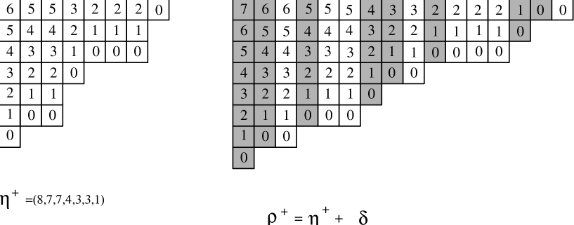
Figure 2: Leg-length diagrams of $\eta=(87^{2}43^{2}1)$ and $\rho^{+}=\eta^{+}+\delta$ for $N=9$

To see where such nodes lie, it is convenient to visualize $\rho^{+}$ obtained from $\eta^{+}$ by inserting the columns of the staircase partition $\delta$ between the columns of $\eta^{+}$ such that the column lengths are weakly decreasing. If one considers the columns of $\delta$ to be placed to the left of the columns of $\eta^{+}$ of the same length (these are the shaded columns in fig. 2), then it is clear that the leg lengths of the nodes $s=(i,j)\in\eta^{+}$ remain unchanged. However their arm lengths increase by the number of columns of $\delta$ with column lengths between $i$ and $(\eta^{+})_{j}^{\prime}-1$ i.e. by $(\eta^{+})_{j}^{\prime}-i=l(s)$ ($(\eta^{+})^{\prime}$ denotes the partition conjugate to $\eta^{+}$). Thus (3.21) is satisfied and we have

$$d_{\rho^{+}}(\alpha)=(1+\alpha)^{|\eta|}\>h_{\eta^{+}}(\alpha/(\alpha+1))\;\gamma_{\delta,\eta^{+}}$$ (3.22)

with

$$\gamma_{\delta,\eta^{+}}=\prod_{(i,j)\in\delta}\left(\alpha(a(i,j)+\eta^{+}_{i}-\eta^{+}_{N-j+2})+l(i,j)+1\right)$$

Finally, the diagram of $\rho^{R}$ is just given by the inverted diagram of $\rho^{+}$. It is clear that the arm length of the nodes remain the same, while (due to the definition (2.8)) the leg-length of the inserted columns of $\delta^{R}$ increase by one (see fig. 3). Similar considerations as above imply

$$d^{\prime}_{\rho^{R}}(\alpha)=(1+\alpha)^{|\eta|}\>d^{\prime}_{\eta^{+}}(\alpha/(\alpha+1))\;\gamma_{\delta,\eta^{+}}$$ (3.23)

By using (3.19), (3.22), (3.23) along with the fact that

$$\frac{e_{\delta}(\alpha)}{e^{\prime}_{\delta}(\alpha)}=\frac{1}{N!}\frac{\prod_{j=1}^{N}(j\alpha+N)}{(1+\alpha)^{N}}=\frac{1}{N!}\frac{{\cal N}^{(P)}_{0}(\alpha/(\alpha+1))}{{\cal N}^{(P)}_{0}(\alpha)}$$

we complete the reconciliation of (3.17) and (3.18).

In addition, taking the ratio of (3.22) and (3.23) provides a simplification of $h_{\eta^{+}}(\alpha/(\alpha+1))/d^{\prime}_{\eta^{+}}(\alpha/(\alpha+1))$ and thus a simplification of the formula in Proposition 3.6.

Proposition 3.6^′ The constant $c_{\rho}$ in (3.1) is given by

$$c_{\rho}=(-1)^{N(N-1)/2}\>\frac{d^{\prime}_{\rho}(\alpha)}{d^{\prime}_{\rho^{R}}(\alpha)}$$

Remark.  In the case $\rho=\rho^{R}$, this gives $c_{\rho}=(-1)^{N(N-1)/2}$, which is a result contained in ref. [1, lemma 2.1].

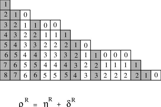
Figure 3: Leg-length diagram for $\rho^{R}$

References

[1]
T. H. Baker, C. F. Dunkl, and P. J. Forrester, “Polynomial eigenfunctions
of the Calogero-Sutherland-Moser models with exchange terms”,
Proceedings of the CRM Workshop on Calogero-Sutherland-Moser models,
Montreal, March 1997.
[2]
T. H. Baker and P. J. Forrester, “The Calogero–Sutherland model and
generalized classical polynomials”, solv-int/9608004, to appear in
Comm. Math. Phys.
[3]
T. H. Baker and P. J. Forrester, “Non–symmetric Jack polynomials and
integral kernels”, q-alg/9612003, to appear in Duke J. Math.
[4]
T. H. Baker and P. J. Forrester, “The Calogero–Sutherland model and
polynomials with prescribed
symmetry”, Nucl. Phys.B 492 (1997), 682–716.
[5]
C. F. Dunkl, “Intertwining operators and polynomials associated with the
symmetric group”, to appear in Monat. Math.
[6]
F. Knop and S. Sahi, “A recursion and combinatorial formula for Jack
polynomials”, q-alg/9610016.
[7]
M. Lassalle, “Polynômes de Jacobi généralisés”, C. R.
Acad. Sci. Paris, t. Séries I312 (1991), 425–428.
[8]
I. G. Macdonald, “Hypergeometric functions”, Unpublished manuscript.
[9]
I. G. Macdonald, Symmetric functions and Hall polynomials,
2nd ed., Oxford University Press, Oxford, 1995.
[10]
E. M. Opdam, “Harmonic analysis for certain representations of graded
Hecke algebras”, Acta Math.175 (1995), 75–121.
[11]
S. Sahi, “A new scalar product for nonsymmetric Jack polynomials”,
Int. Math. Res. Not.20 (1996), 997–1004.
[12]
R. P. Stanley, “Some combinatorial properties of Jack symmetric
functions”, Adv. in Math.77 (1989), 76–115.