On the mechanism of decadal oscillations in a coarse resolution ocean model

Abstract

The mechanism that causes an interdecadal oscillation in a coarse resolution sector ocean model forced by mixed boundary conditions is studied. The oscillation is characterized by large fluctuations in convective activity and air/sea heat exchange on a decadal time scale. When the convective activity is large, a strengthening of the southeastward surface flow advects more relatively fresh water from the northwestern part of the basin into the convective area, which reduces the convective activity. Similarly, when the convective activity is small, the flow of relatively fresh water is weak, which enables the expansion of the convective area. The periodically strengthening and weakening of the southeastward surface flow at the polar boundary of the basin is revealed by a negative polar cell in the meridional overturning. The existence of a halocline and an inverse thermocline with cool and fresh water above a warm and salty subsurface is essential for the oscillation. Further, the oscillation critically depends on how the ocean circulation, and especially the surface circulation, responds to anomalous convective activity. Horizontal boundaries turn out to play an important role in the dynamical response of the ocean circulation. That the dynamical reponse is essential to the oscillation is confirmed with two simple (conceptual) models, and some idealized ocean experiments. Finally, the sensitivity of the oscillation to salt perturbations and the restoring constant for the air/sea heatflux is investigated.

1 Introduction

In order to determine whether the increasing concentration of greenhouse gases is affecting our climate one needs to have a clear picture of natural climate variability. It has since long been argued that a considerable part of natural climate variability on decadal and longer timescales is due to variability of the ocean circulation (Bjerknes 1964; Broecker 1985, Kushnir 1993). In particular the density driven ocean circulation called thermohaline circulation (THC) is thought to be responsible for a substantial part of the natural climate variability on decadal and longer time scales.

The THC is driven by fluxes of heat and freshwater at the oceans surface. The freshwater flux is caused by evaporation, precipitation, river run off and sea-ice melt or accretion. The net effect of these fluxes on the surface salinity is often accounted for by a virtual salinity flux. Simple parameterizations of these heat and salt fluxes are often used to investigate the variability and stability of the THC. Often used are the so-called mixed boundary conditions (MBCs), consisting of a fixed salt flux and a time varying heat flux which restores the sea surface temperature (SST) towards an apparent atmospheric temperature. Commonly used values of the restoring constant are 50 W m^-2 K^-1 (Haney 1971) or even higher, which usage actually pins the SST down to the prescribed atmospheric temperature. MBCs reflect that there is a direct feedback between the SST and the heatflux, whereas a direct feedback between the sea surface salinity (SSS) and the freshwater flux does not exist. However, relatively large errors in the heatflux may occur as, using MBCs, the SST is forced towards a fixed atmospheric temperature, whereas in reality the atmosphere closely adapts to the SST in most areas. On the other extreme, some researchers use a fixed heatflux. This however neglects the possible influence of the ocean on climate variability as the ocean is now basically forced to transport a fixed amount of heat.

With these relatively simple boundary conditions variations of the THC on decadal and longer time scales were obtained. In this study we will concentrate on the (inter)decadal time scale. Weaver and Sarachik (1991) (hereafter WS91) first found decadal variability in an ocean model forced by MBCs. Thereafter many others also reported oscillations using different boundary conditions and models (Chen and Ghil 1995; Greatbatch and Zhang 1995; Cai 1995; Weisse et al. 1994; Weaver et al. 1993 (hereafter Wea93); Myers and Weaver 1994, Moore and Reason 1993; Huang and Chou 1994; Yin and Sarachik 1995 (hereafter YS95); Drijfhout et al. 1996). Decadal variability was also found with the inclusion of a thermodynamical sea ice model (Zhang et al. 1995; Yang et Neelin 1994).

Most of the current research concentrates on the development of boundary conditions which parameterize the atmospheric feedbacks more realistically, and the investigation of the stability and variability of the THC using these boundary conditions (Rahmstorf 1994; Cai and Godfrey 1995; Chen and Ghil 1995). Although we recognize the importance of this we decided not to pursue this approach in this paper. We feel that a clear picture of the mechanisms causing decadal variability using simple boundary conditions is still lacking, and that such a picture could be helpful in understanding the oceans behavior when the atmospheric feedbacks are represented more properly.

Using fixed heat and/or salt fluxes several authors (Huang and Chou 1994; Greatbatch and Zhang 1995; Cai 1995, Chen and Ghil 1994) have noticed the similarity between different forms of variability. Greatbatch and Zhang (1995) first noticed the similarity of their oscillation using fixed heat and salt fluxes with an oscillation obtained in a globally coupled model (Delworth et al. 1993). Although there is not yet a complete and clear picture of the mechanism of these oscillations, there is a growing consensus that these oscillations are basically caused by the same mechanism. For MBCs however the picture of the mechanisms causing interdecadal variability is more confusing. Weaver and Sarachik (1991) explain their oscillation by the advection of a positive salt anomaly interacting with convection. Yin and Sarachik (1995), however, argue that the same oscillation is mainly set by a stabilizing flow of relatively fresh water from the polar boundary, and the destabilizing influx of relatively warm water below the surface into the convective area. In Moore and Reason (1993) a more complicated mechanism of their oscillation is sketched where convection combined with a strong negative feedback of anomalous advection of fresh water in the surface layer and salty water at a larger depth plays a role. They argue that a dynamical interaction between the convective activity and the strength of the surface flow is essential, whereas Yin and Sarachik (1995) are ambiguous on this point. Finally, Zang et al. (1995) argue that their oscillation is caused by the thermal insulation effect of sea-ice.

It is tempting to question whether or not the mechanism causing oscillations with MBCs are really so different. But before being able to answer this question one should have a clear conceptual picture of the mechanisms causing oscillations. With this paper we aim to establish a clear picture of the mechanism causing the oscillation in WS91. This oscillation has also been studied in WS93 and in YS95. Large variations in convective activity and the air/sea heat flux are characteristic of this oscillation. The oscillation turns out to be mainly driven by convection and advection. The impact of convection and advection on the heat and salt budgets of the convective area is carefully estimated. Our analysis indicates that the oscillation crucially depends on how the surface flow responds to anomalous convective activity. The advection by the surface flow of fresh water into the convective area mainly determines the convective activity. We show that the period of the oscillation is mainly determined by the timescale of this advective feedback.

In this paper we do not describe a new mechanism. Several processes and feedbacks that are potentially important are already mentioned in literature. Our aim is to clarify the role of these feedbacks and processes, and to complete the picture of the mechanism as far as possible. Yin and Sarachik (1995) already gave a quite extensive description similar to ours of many important processes. Our conclusions however differ from theirs mainly concerning the question what determines the time scale and the amplitude of the oscillation, and we will therefore focus on these differences. Our description of the response of the surface flow to anomalous convective activity also shows a large resemblance with the mechanism described by Moore and Reason (1993). Finally, several authors (Winton 1996a; Greatbatch and Peterson 1995) also proposed that boundary waves might play a role. This aspect of the oscillation is also studied in this paper.

Besides the question concerning the mechanism of the oscillation, information about the sensitivity and robustness of the oscillation (to changes in parameter values, forcing, inclusion of other processes like sea-ice and/or atmospheric feedbacks, atmospheric noise or perturbations) is important. Two of our experiments shed some light on this. We show that the oscillation is fairly insensitive to perturbations in the surface salinity. This contrasts highly with the sensitivity of steady states obtained by a spin-up with restoring conditions. With MBCs these steady states usually show a high sensitivity to surface salinity perturbations, and a polar halocline catastrophy is easily invoked. Furthermore, we show that the oscillation is rather insensitive to the restoring constant for the surface temperature. Our results on this point agree with those in YS95.

The contents of the paper is as follows. In section 3 we reproduce the oscillation of WS91, and in section 4 a detailed analysis of the oscillation is given. In section 5 several sensitivity runs are performed. A comparision with the results of Yin and Sarachik (1995) is made in section 6. A summary and conclusions are given in section 7. In the appendix we investigate the possibility of convective oscillations in a two box model.

2 The model

The ocean model used is basically a ”GFDL” type model. It uses the usual budget equations for temperature, and salinity with diffusion parameterizing the eddy-transports. The momentum equations are split in a barotropic and a baroclinic part. For the barotropic part the ”Sverdrup-balance” is solved (see Lenderink and Haarsma 1994, hereafter LH94). As we use a flat bottomed ocean the barotropic part is completely determined by the windstress only. The equations for the baroclinic velocity field are solved in time. An asynchronous time integration (Bryan 1984) is used to slow down internal gravity and Kelvin waves. In Wea93 and YS95 it has been shown that the asynchronous time integration does not significantly affect the oscillation. An eddy viscosity is used in both horizontal as vertical direction, whereas the horizontal and vertical advection of momentum is neglected. The equation of state is similar to the one employed in LH94. A convective mixing scheme is employed after each timestep. It is the standard mixing scheme as employed in the GFDL Bryan-Cox code. Starting from the surface level the densities of each pair of levels (first level 1 and 2, then level 3 and 4 etc.) are compared and the levels are mixed completely in case of an unstable stratification. Thereafter, the procedure is repeated starting from the second level.

The model basin extends from the equator to 64 ^oN and extends 60 degrees in longitudinal direction. The ocean basin is 4000 meters deep and bottom topography is not included. The horizontal resolution is 3.75 ^o in longitudinal and 4.00 ^o in latitudinal direction. The layer thicknesses are (from the surface to the bottom) 40, 40, 80, 140, 250, 350, 400, 450, 500, 550, 600 and 600 meters. The timestep for the ocean model is 4 days. For the horizontal and vertical diffusivity we used $1\;10^{3}$ m² s^-1 and $0.6\;10^{-3}$ m² s^-1 respectively, and for the horizontal and vertical viscosity $2.5\;10^{5}$ m² s^-1 and $1\;10^{-3}$ m² s^-1.

3 The oscillation

3.1 Reproduction of the oscillation

We performed an experiment similar to the experiments described in Wea93 and WS91. First, we spun our model up from rest using restoring conditions We used forcing fields and parameter values similar to the ones used in Wea93 and WS91. The temperature and salinity profile to which the surface is restored, which are the same as in WS91, are shown in Fig. 1. For the restoring timescale we used 20 days. The zonal windstress also equals the profile used in WS91.

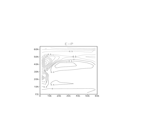
Figure 2: Diagnosed E-P (evaporation - precipitation) flux in m yr^-1.

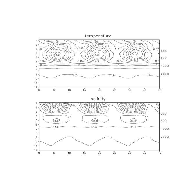
Figure 6: Area mean temperature and salinity and convective fraction as a function of time and depth. At the left-hand side depth in levels, right-hand side depth in meters.

After the system reached its equilibrium state with restoring conditions, we diagnosed the E-P field needed to sustain this state. This field as shown in Fig 2 closely resembles Fig. 2c in Wea93. The spinup state is characterized by deep convection along the polar boundary. Relatively shallow convection up to 1000 meter also occurs at 50 ^oN. The meridional overturning circulation as shown in Fig 3 is very similar to Fig. 6b of Wea93 and consists of a positive overturning cell of 13 Sv with sinking motion at the polar boundary. Switching to mixed boundary conditions, this state collapses after a small salinity perturbation (-0.1 psu in one surface gridbox only) in the convective area. Deep convective mixing at the polar boundary vanishes, meanwhile, however, convective activity at lower latitudes increases in strength and the system starts to oscillate on a decadal timescale. We ran the model another 2500 years during which the system continues to oscillate. We analyzed the oscillation after approximately 2000 years of integration.

Fig. 4 and Fig. 5 show the convective activity and the meridional overturning at 6 times during the oscillation. We start our description at t = 0 years when the convective activity is strong. A relatively weak positive overturning cell and a fairly strong negative polar cell are shown. In the next 3 years shallow convective mixing is decreasing, whereas deep convective mixing to the ocean bottom continues. At the same time both negative and positive overturning cell increase in strength. Shortly after t = 4 years deep convective mixing disappears completely. The negative overturning cell collapses in one year time, and the maximum of the overturning displaces to the polar boundary. Shallow convection starts again only a few years after the collapse of the negative cell, shortly before t = 6 years. In the following years, first a spreading of the convective area and a decrease in strength of the positive overturning cell, and then a gradual retreat of the convective area, a deepening of convective mixing at the northeastern corner and an increase in strength of the overturning cell is observed. During these years the polar cell monotonically increases in strength. After 13 years the circulation approximately equals the circulation at t = 0 and a new cycle starts.

3.2 A simple area mean picture

Fluctuations in convective activity are a dominant feature of the oscillation. In response to the convective activity the atmospheric heatflux and also the oceanic meridional heat transport display large variations (see below and also WS91). We therefore concentrate on the area A_con indicated in Fig. 4. The area A_con is approximately the smallest rectangular enclosure of the area where the convective activity changes during the oscillation. In Fig. 6 we show the area mean temperature and salinity as a function of depth and time. In this figure we also plotted the time evolution of the convective fraction. Here, the convective fraction is defined as the area affected by convective mixing at a certain depth divided by the total area A_con. It is shown that the strongest fluctuations in temperature and salinity occur in the upper 700 meters of the ocean. The main convective activity is confined to the upper 1000 meters. In the upper 600 meters about 90 % of the area is affected by convection, and between 600 and 1000 meters still 60 % of the area is affected. Below 1000 meters, however, this measure sharply decreases to about 20 %. In the following we will therefore concentrate on the upper part of the ocean. Figure 6 shows a warm subsurface and a fresh surface ocean in the nonconvective phase. In this phase the salinity gradient (halocline) keeps the ocean stably stratified, whereas the temperature gradient (inverse thermocline) tends to destabilize the stratification. During the convective phase the heat contained by the anomalous warm subsurface ocean is rapidly released to the atmosphere. This heatflux is shown in Fig. 7. At the same time the surface becomes considerably saltier.

In order to investigate which processes dominate the evolution in the convective area A_con we defined a surface and a subsurface box in A_con and investigated their evolution in time. The surface box $B_{u}$ consists of the uppermost three levels (0-160 m) and the subsurface box $B_{l}$ consists of the next two levels (160-550 m). We have chosen these levels for $B_{l}$ because in the nonconvective phase these levels contain the major part of the heat that is subsequently given off to the atmosphere in the convective phase.

We plotted in Figs. 8a,b the mean temperature and salinity for both boxes. The large variations in the surface (of $B_{u}$) salinity and the subsurface (of $B_{l}$) temperature are again clearly visible. We focus on the cause of these variations. Thereto, we plotted in Figs. 8c,d the time derivative of the surface salinity and the subsurface temperature. We also plotted the contribution of horizontal advection and convection. Figure 8c shows that horizontal advection and convection almost completely determine the surface salinity balance. Horizontal and vertical diffusion (not shown) are of only of secondary importance when considering the box averaged values, although locally they could play a role. The surface heat balance is mainly determined by convection and the atmospheric heatflux (not shown). The atmospheric heatflux keeps the surface temperature close to the atmospheric temperature. The fluctuations of the surface box temperature are mainly caused by the contribution of the temperature of level 3 – which is less affected by the surface heatflux – to the box mean. For the subsurface box $B_{l}$ horizontal advection provides for a nearly constant source of heat and salt. These heat and salt fluxes are mainly due to the meridional overturning which advects heat and salt from the equator northward just below the surface. In the absence of convection the temperature and salinity of the subsurface rise due to this term. When convective activity is large the convective flux however causes a decrease in the subsurface temperature and salinity.

A relatively simple picture of the dominant processes in the convective area now emerges. First, consider t = 0, when the convective activity is large. At this time an increasing amount of fresh water due to horizontal advection enters the surface box. The area with convection is decreasing in response to the increasing advection of fresh water water into the convective aea. The surface salinity decreases further because of the decreasing amount of salt mixed up by convection. At the same time a gradual warming of the subsurface ocean is observed because the heat entering the subsurface by horizontal advection is no longer released to the atmosphere in the area where convection is suppressed. The nonconvective part of the box is therefore responsible for the rise in the box mean temperature. After 5 years convection is completely suppressed by the flow of relatively fresh water entering the surface box. Shortly thereafter, the anomalous flow of fresh water breaks down (see also Fig. 5), and the advection of salt becomes for a short time even positive. The resulting rise in surface salinity quickly re-enables convection. As will be discussed below, the positive feedback of convection in an ocean with relatively warm and saline water beneath a fresh and cool surface layer now results in a rapid growth of the convective area. This rapid growth is revealed by the sharp rise in the convective salt source for the surface box from 6 to 8 years. The convective area now starts to decrease again due to the cooling of the subsurface box and the increasing advection of fresh water into the surface box.

4 The Mechanism

In this section we will explain the mechanism of the oscillation. The processes responsible for the expansion and retreat of the convective area are studied. By definition, fluctuations in convective activity are caused by changes in the vertical temperature and salinity gradient. We focus on the surface salinity and the subsurface temperature because these contribute most to the variations in the density gradient. In the first subsection we will consider the role of the subsurface temperature and surface salinity. We will argue that, with a steady ocean circulation that does not respond to the fluctuations in convective activity, convection is self-sustaining and that changes in the subsurface temperature and surface salinity do not cause oscillatory behavior. We therefore propose that ocean dynamics play a role. In the second subsection we will show in a conceptual model that changes in the surface advection due to the ocean dynamics can give rise to oscillations in convective activity. Finally in the third and the fourth subsection we will investigate the dynamic reponse, and the associated changes in advection, during the convective and the nonconvective phase, respectively.

4.1 The expansion and retreat of the convective area.

The role of the subsurface temperature can be summarized as follows. First consider the retreat of the convective area. Convection is suppressed only after the heat anomaly contained in the subsurface ocean is released to the atmosphere. With a warm subsurface ocean convection continues because of the unstable temperature gradient. In this case a typical heat anomaly is released in two year time, where we used a layer thickness of 400 m, a temperature anomaly of 2 ^oC, and an atmospheric heat flux of 50 W m^-2. Similarly, the warming of the subsurface during the nonconvective phase is a precondition for the triggering of convection. This warming of the subsurface during the nonconvective phase is somewhat slower than the cooling during the convective phase, but still relatively fast.

When convection starts in the northeastern corner, convection mixes up a large amount of heat and salt to the surface. The heat is rapidly lost to the atmosphere, whereas the surface salinity remains high, and becomes a source of salt for the surrounding ocean. The mixing of salt to the surface and the subsequent horizontal spreading due to advection and diffusion, cause – in concert with the relatively low influx of fresh water by advection – a rapid expansion of the convective area. Due to the convective feedback, the expansion of the convective area even continues a short time while the advection of fresh water is already increasing. Thereafter, the net advection of fresh water into the convective area increases due to the increasing southeastward surface velocity and the increased surface salinity gradient. The increased advection of fresh water causes a reduction of the convective activity, and eventually establishes a complete suppression of convection.

In the appendix we show that convection is locally self-sustaining. With a steady, not responding to the convective activity, circulation convective activity will not oscillate. The mechanism proposed in Yin (1995, see also section 6) does not operate in that case: Within a reasonable parameter regime, the subsurface warming when convection is off is not large enough to trigger the onset of convection; when convection is on, the surface freshening due to the increased surface salinity gradient is not large enough to suppres convection. Instead locally two states – a convective and a nonconvective – exist and hysteresis occurs (see also LH94, LH96). This leaves us with the question why the system oscillates. We propose that the ocean dynamics, and especially the changes in the surface advection of salt caused by the ocean dynamics, play an important role. In the next paragraph we will first investigate the role of ocean dynamics in a conceptual model. Thereafter, we will investigate it in the ocean model.

4.2 A conceptual model for the oscillation

The conceptual model is shown in Fig. 9. It consists of two boxes: a surface box with salinity $S$ and a subsurface box with temperature $T$. The temperature of the surface box and the salinity of the subsurface box are kept constant in time. Convective mixing with a strength $C$ occurs between the boxes. Furthermore, a polar overturning cell with strength $O$, which advects relatively fresh water into the convective area, is shown. The system is linearized around a mean convective state, and $T$, $S$, $C$ and $O$ are therefore anomalous variables.

Let us first consider the effect of the subsurface temperature in isolation. The subsurface temperature will rise when the convective activity is low due to the advection of warm water by the meridional overturning, and fall when the convective activity is high:

$$\frac{dT}{dt}=-\theta C,$$

where $\theta$ is a positive constant. The convective activity on the other hand is dependent on the subsurface temperature. It will be high when the subsurface temperature is high:

$$C=\kappa T,$$

where $\kappa$ is a positive constant. Solving this system yields a damped exponential. The mechanism of the decay is simple: convection causes a cooling of the subsurface, which reduces the convective activity further. This feedback will be called the convective temperature feedback.

We continue with the surface salinity. If we consider the effect of convection in isolation a growing exponential is obtained in a similar way. In words, convection mixes salt up to the surface; the resulting increase in surface salinity destabilizes the stratification further and causes an increase in convective activity. This feedback will be called the convective salinity feedback.

Within this conceptual model, the convective temperature and salinity feedback generate decay and amplification of the convective activity, respectively. They are unable to generate oscillatory behavior. This is because there is no time lag between the convective fluxes and the convective activity. The essential time lag is provided by the advection of relatively fresh water into the convective area in response to changes in convective activity. This advective feedback can be described as follows. The strength of the polar cell increases when the convective activity is anomalously high:

$$\frac{dO}{dt}=\zeta C.$$

Furthermore, the advection of relatively fresh water into the convective area by $O$ is represented by

$$\frac{dS}{dt}=-\gamma O,$$

and the convective activity is related to the surface salinity by

$$C=\sigma S.$$

In these equations $\zeta$, $\gamma$ and $\sigma$ are all positive constants. Solving this system yields a second order ordinary differential equation:

$$\frac{d^{2}O}{dt^{2}}+\zeta\gamma\sigma O=0.$$

The solution of this equation is a harmonic oscillation with a time scale 2$\pi$/$\sqrt{\zeta\gamma\sigma}$. From the data of the ocean model we estimate $\sigma=1$ (psu)^-1 – the convective activity is normalized –, $\zeta$ = 3 Sv yr^-1, and $\gamma$ = 0.1 psu (Sv yr)^-1. This gives a time scale of 11 years. The estimates for the parameters are obviously not very precise, but the (inter)decadal time scale seems nevertheless robust. The physical picture of the oscillation is:

…weak convective activity $C$ $\rightarrow$ slow overturning $O$ and weak advection $\rightarrow$ high surface salinity and strong convective activity $C$ $\rightarrow$ fast overturning $O$ …

The systems oscillates because there is a phase lag between the convective activity and advection of fresh water into the convective area. This phase lag is clearly shown with the retreat of the convective area. The maximum in convective activity occurs between 10 and 12 years – in Figs. 8 c,d the convective fluxes are maximal at t = 10 years; the convective fraction $q$ in Fig. 6 is maximal after 12 years. The maximum in the advection of fresh water in Fig. 8 c occurs approximately one quarter period later, at t = 15 years. The phase lag is however not so evident when the convective activity reaches its minimum at t = 5 years: the maximum in the advection of salt at t = 6 years in Fig. 8 c only lags the minimum of convective activity about one year. This is due to the occurrence of a fast boundary wave, which will be discussed in the following.

In the next two paragraphs we will focus on the dynamical response of the ocean model, in particular the dynamical response of advection, during two phases of the oscillation. In the first paragraph we will focus on the convective phase, and in particular the end of the convective phase during which the convective area retreats. In the second paragraph we will focus on the nonconvective phase.

4.3 Advection during the convective phase

To complete the picture of the mechanism of the oscillation, the relation between convective activity and the net advection of fresh water into the convective area has to be established. In this section we will discuss this relation during the convection phase. We will focus on the period during which the convective area retreats.

The net advection of fresh water is determined by both the surface salinity gradient and the strength of the flow. The surface salinity gradient is established by two effects. First, precipitation creates a pool of fresh water outside the convective area mainly in the northwestern corner of the basin. Second, convection is responsible for a positive salinity anomaly in the convection area. In the convective phase both the surface salinity gradient and the southeastern surface flow increase. In order to estimate the contribution of changes in the strength of the surface flow and changes in the surface salinity gradient seperately, we divided the surface velocity into a time mean $v_{m}$ and an anomalous part $v^{\prime}$. We computed the net advection by the mean velocity and the anomalous velocity. The changes in the advection of fresh water by the mean flow $v_{m}\cdot\nabla S$ represents the changes due to surface salinity changes only. We denote the response of $v_{m}\cdot\nabla S$ to anomalous convective activity shortly by the static response of advection, because it is the response in an ocean with fixed, not responding to anomalous convective activity, velocities. The net advection by the anomalous velocity $v^{\prime}\cdot\nabla S$ is the dynamic response of advection, which is due to changes in the strength of the flow.

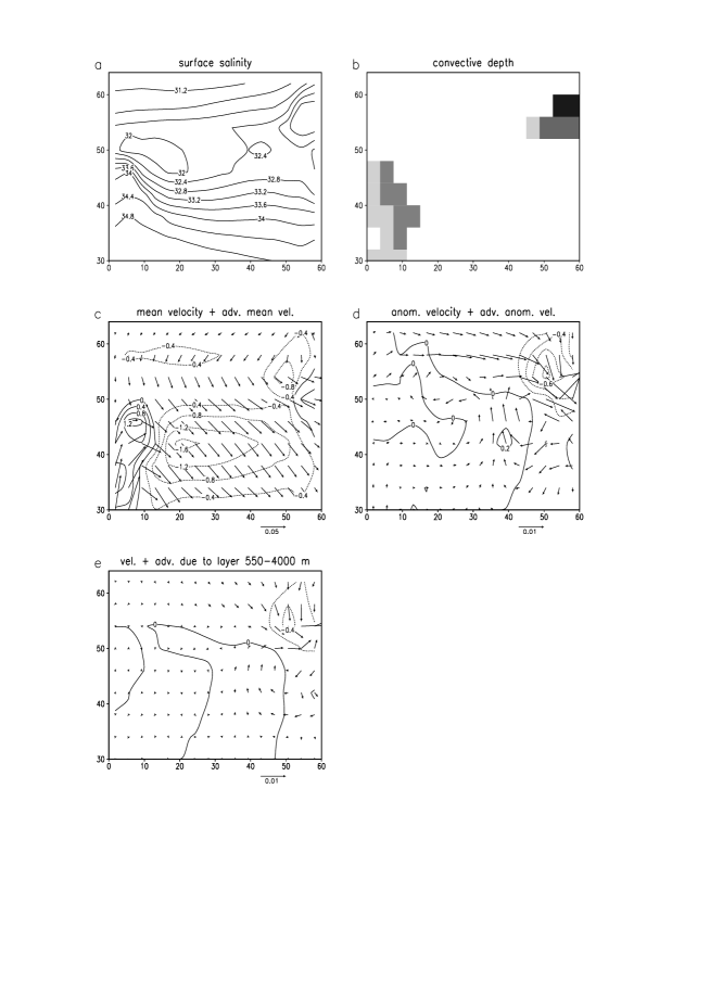
Figure 11: Similar to Fig. 10 but than for t = 4 years. Also shown are the anomalous velocity due to the density anomaly beneath 550 m, and the advection due to this velocity (e).

We concentrated on two times, t = 0 and t = 4, during the retreat of the convective area. At t = 0 the convective area is still relatively large. In Fig. 10 a,b the SSS and the convective activity are shown. In Fig. 10 c,d we plotted $v_{m}$ and $v^{\prime}$, and the horizontal advection due to these velocities: $v_{m}\cdot\nabla S$ and $v^{\prime}\cdot\nabla S$. Both $v_{m}$ and $v^{\prime}$ advect fresh water into the southern part of the convective area; the contribution of $v_{m}$ to the advection is about about two to four times larger than the contribution of $v^{\prime}$. The southeastern direction of the mean flow $v_{m}$ is due to a combination of the windstress, which mainly forces the southward component of the flow, and the density gradient caused by dense water trapped along the northern boundary of the basin, which mainly forces the eastward component of the flow. For t = 4 the convective area is only small with deep convection near the northeastern corner. As shown in Fig. 11 the anomalous southward flow clearly points into the convective area now, whereas at t = 0 years the anomalous flow was mainly parallel with the convective border. The horizontal flow is consequently more efficient in causing a freshening of the convective area. Both $v_{m}$ and $v^{\prime}$ now contribute almost equally to the advection into the convective area.

It is shown that the dynamic response of the advection of fresh water is large at the end of convective phase. During most of the time however the static response dominates. In addition, horizontal diffusion (see YS95) has approximately the same effect as the static response of advection. Because the dynamic response of advection seems to be so small compared to the static response and horizontal diffusion, it could be argued that the dynamic response is not essential. The results of our conceptual model indicate that this is not the case. The formulation of the advective feedback in our conceptual model can be considered to represent the dynamic response of advection linearized around a mean salinity gradient. The phase lag between the advection of fresh water and the convective activity causes the oscillatory behavior. Since convection is a fast process, the horizontal salinity gradient is almost in phase with the convective activity. The static response of advecton is therefore approximately in phase with the convective activity, and does not give rise to oscillatory behavior. In the following we will therefore concentrate on the cause of the anomalous velocities.

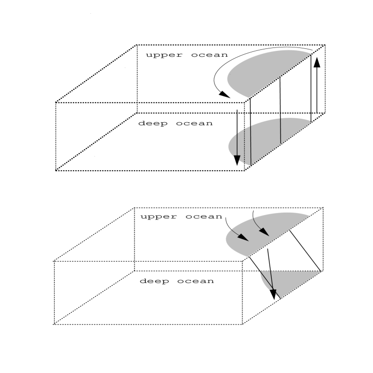
Figure 12: Sketches of the relationship between convection, density anomalies, and anomalous velocity fields. The density anomaly is depicted by the dashed area. Anomalous velocities are shown by the arrows.

In order to get some feeling for the response of the circulation to changes in convective activity we first consider the following idealized situation. Suppose that we have the following idealized situation with uniform anomalous convective activity in a certain area of the ocean and that this convective activity causes an uniform density anomaly in this area. Further, assume that advective processes did not yet displaced the density anomaly. This situation is schematically depicted in Fig.12 a. If we assume geostrophy, which is nearly perfectly fulfilled on the scales considered, the anomalous surface velocity associated with the density anomaly is a cyclonic circulation along the boundary of the convective area. At depth the direction of flow is reversed. Upwelling at the western boundary just north of the convective area, and downwelling just south of the convective area now close the circulation. In this situation, the anomalous surface flow would therefore be parallel with the convective border and would not advect fresh water into the convective area. The dynamic response of advection is therefore zero in this situation.

It is obvious that at the end of the convective phase our model is not in the idealized situation sketched above. At t = 4 years the the anomalous velocities are clearly directed into the convective area. Based on data of the ocean model, we sketched in Fig. 12b the situation that is more appropriate for the end of the convective phase. In this situation horizontal advection caused a displacement of the density anomaly at depth. This is for example visible at a depth below 1000 m (not shown) where a dense, negative temperature anomaly is trapped in the northeastern corner of the basin. Associated with the density anomaly is also a surface circulation that is directed into the convective area (see also Fig. 11e below). Besides horizontal advection, also vertical advection plays a large role in causing anomalous densities. Anomalous downwelling in a stratified ocean causes a negative density anomaly; similarly, anomalous upwelling causes a positive density anomaly. Therefore, the anomalous downwelling at the eastern boundary just south of the convective area in Fig. 12 a causes a negative density anomaly. Anomalous upwelling at the border of the convective area similarly creates a positive density anomaly north of the convective area. The importance of upwelling in creating horizontal density and thus velocity anomalies has also been appreciated by Moore and Reason (1993). In our case, the anomalous upwelling near the polar boundary during the convective phase, which is for example revealed by the pictures of the meridional streamfunction, causes a positive density anomaly at the northern boundary. This density anomaly causes an easterly surface velocity into the convective area.

In order to quantify the role of density changes at different depths in causing surface velocity anomalies, we used the following diagnostic tool. Anomalous velocity fields are computed from the anomalous density field using the assumption that the ocean circulation is in geostrophic balance. Because the ocean is to a very high degree geostrophic the anomalous velocity fields obtained from this procedure and the observed anomalous velocity field are almost indistinguishable. Then we computed the anomalous surface velocity due to density anomalies at different levels of the ocean. Performing this procedure for the anomalous density below 550 m, we obtained the results as depicted in Fig. 11e. It is shown that about 60 % of the southeastward velocity near the northeastern corner, and consequently about 60 % of the horizontal advection of fresh water into the convective area is due to the density changes below 550 m. The oscillation is therefore not only a surface and subsurface phenomenom; also changes at depth are important in determining the dynamical reponse of the ocean model. We also performed this procedure for t = 0 years. It turned out that the major part of the anomalous velocities is due to the density changes in the upper few hundred meters of the ocean. The anomalous flow only has a small component into the convective area, and transported therefore only few fresh water into the convective area.

4.4 Advection during the nonconvective phase

It is already shown in Fig. 5 that during the nonconvective phase the negative overturning cell at the polar boundary collapses. This is due to the occurrence of a boundary Kelvin wave. Kelvin waves have been observed in several studies of variability in coarse resolution ocean model, and some authors claim their essential role for variability. (Winton 1996a; Greatbatch and Peterson 1995). Strictly speaking this wave is not resolved in coarse resolution ocean models, however, these models do generate a numerical wave with equivalent characteristics (Winton 1996a). In a strongly stratified equatorial ocean the propagation speed of this wave is fast. In the weakly stratified polar ocean however the wave considerably slows down and could be responsible for decadal variability.

The physics of this wave can be understood as follows. Consider an area with downwelling at the eastern boundary in a stratified ocean. This introduces a local density minimum by the downward advection of lighter water. The negative density anomaly introduces a cyclonical circulation at depth and an anti-cyclonical surface circulation. The corresponding vertical circulation at the boundary with upwelling south and downwelling north of the anomaly, now leads to a northward displacement of the downwelling area. In a stratified ocean the wave therefore travels cyclonically around the basin.

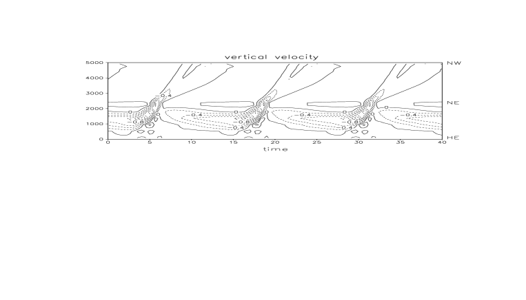
Figure 13: Time development of vertical velocity at 1000 m as a function of distance (km) along the boundary. HE corresponds to 32 ^oN along the eastern boundary, NE the northeastern corner, and NW the northwestern corner of the basin.

To illustrate the propagation of the Kelvin wave, we plotted in Fig. 13 the vertical velocity as a function of time along part of the boundary. This part consists of the polar part of the eastern boundary (HE to NE in Fig. 13) and the polar boundary (NE to NW). The vertical velocity occuring at the boundary is for a large part responsible for the zonally integrated vertical mass transport as depicted in plots of the meridional overturning. From t = 0 to t = 4 the downwelling 1000 km south of the polar boundary is clearly visible. When after 5 years deep convection at the northeastern boundary stops, the downwelling area starts to travel cyclonically along the boundary. In about two years time the wave reaches the polar boundary, which is also revealed by the collapse of the negative, polar overturning cell in Fig. 5. Thereafter the wave travels along the polar boundary to the west, while slowly reducing in strength. The time scale of the wave propagating along the boundary is about five years.

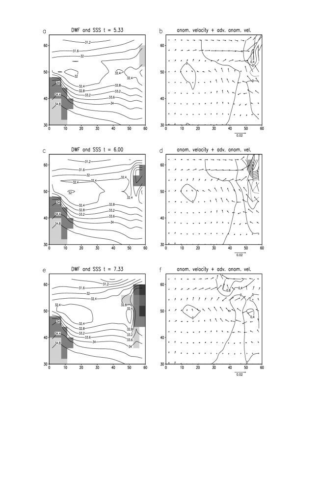
Figure 14: Surface salinity, deep-water formation, anomalous surface velocity, and surface salt advection (psu yr^-1) due to anomalous velocity during the weak convective phase.

The effect of the Kelvin wave on the ocean dynamics, in particular the advection of salt at the surface, is illustrated in Fig. 14. Figure 14 shows the surface salinity, convective depth, anomalous velocity, and surface salt advection due to the anomalous velocity are shown for three different times, t = 5.33, t = 6.00 and t = 7.00 years. At t = 5.33 years, the Kelvin wave is still located at the eastern boundary, approximately at 56 ^oN. The anti-cyclonical surface circulation at the eastern boundary associated with the Kelvin wave advects relative saline water northward. This rapidly turns convection on – in the appendix it is argued that a change in the surface velocity is necessary for the re-initialization of convection. At t = 6 years, the boundary wave is located in the northeastern corner of the basin, and one year later it is about halfway the northern boundary. Associated with the propagation of the Kelvin, the strong eastward surface flow along the northern boundary of the basin turns into a weakly western flow. With the relatively weak (south)eastern surface flow, or even westerly flow, the convective area expands rapidly. Thereafter, the eastern surface flow starts to increase again. To summarize, the role of the Kelvin wave is mainly twofold: First, the northward surface flow associated with the wave re-initializes convection rapidly after its suppression. Second, it resets the ocean from a state with the strong, (south)eastern surface flow to a state with a weak surface flow, so that the convective activity is able to expand rapidly. The dynamical response of the ocean during the nonconvective phase is therefore dominated by the Kelvin wave. On the other hand, the role of Kelvin waves during the convection phase seems to be minor. We could not find any evidence of wave activity during this period.

The suggestion of Winton (1996a) that the Kelvin wave, when it reaches the energetic western boundary current, influences the overturning and therefore modifies the advection of heat and salt from the south into the convective area seems not likely. In the previous section it was shown that the suppression of convection is mainly due to the anomalous advection of fresh water from the northwest into the convective area. Furthermore, Wintons hypothesis implies that the suppression of convection is due to the slow down of the positive overturning circulation (because the overturning advects salt into the convective area) while actually an increase in strength of the positive overturning cell is observed between t = 0 and t = 4 years. We therefore conclude that boundary waves play a role in the sense that they cause the rapid re-initialization of convection and reset the strong (south)eastern surface flow at the end of the convective phase, which enables the convective area to expand. There are no indications that the suppression of convection is due to boundary waves. The underlying physics responsible for the propagation of the wave are however important during the whole cycle of the oscillation. Density anomalies due to anomalous upwelling and downwelling at the boundary determine for a large part the dynamic response of the advection of fresh water into the convective area. Boundaries therefore play an important role in the mechanism of the oscillation.

4.5 Experiments with fixed velocity fields

To confirm once more that a dynamical response of the ocean model to anomalous convective activity is essential, we performed a few idealized experiments with the ocean model. Thereto, we ran the ocean model with stationary velocity fields. For the velocity fields we used the mean velocity field and also two instantaneous, diagnosed velocity fields. As a measure of the convective activity we show the integrated heatflux in Fig. 15. For the first experiment we first integrated the model during two periods forward in time, and then switched over to the mean velocity field. For the other two experiments we integrated the model to t = 10 years and to t = 15 years respectively, and then kept the velocity field fixed. These times are chosen because the southeastward velocity at the surface into the convective area are then respectively maximal and minimal. The strength of this flow determines the time scale at which the surface salinity of the convective area tends to approach the salinity of the northwestern corner, which potentially (see the Appendix) could be important for the occurrence of the oscillation. With the velocity fields used a wide range of realistic relaxation time scales is covered. None of these integrations, however, yielded self sustained oscillations in convective activity on a (inter)decadal time scale. After switching to a steady velocity field all runs only showed small variations on a very short time scale. No (inter)decadal oscillations were found. These experiments therefore indicate that ocean dynamics play an essential role in (inter)decadal oscillations.

4.6 Summary of the mechanism

We start the cycle in the phase with weak convective activity. A short time later convection is completely suppressed due to the strong advection of relatively fresh surface water from the northwestern polar boundary into the convective area. When convection stops the downwelling area just south of the convective area at the eastern boundary of the basin begins to travel cyclonically around the basin as a boundary Kelvin wave. The movement of the downwelling area is revealed by a collapse of the negative overturning cell near the polar boundary. The advection of relatively fresh water from the polar area into the convective area breaks down, and convection starts again at the eastern boundary. When convection is off, the subsurface becomes warm and saline compared to the surface due to the influx of heat and salt at depth. In the nonconvective phase this stratification has become very unstable – that is, potentially convective (see LH96) – using MBCs. The relatively weak advection of fresh water (weak southeasterly flow) and the large amount of salt mixed up by the convective patch at the boundary cause a rapid growth of convection. During the subsequent strong convective phase the heat contained in the subsurface ocean between approximately 160 and 600 meter deep is rapidly released to the atmosphere. The cooling of the subsurface tends to stabilize the stratification. At the same time the advective influx of fresh water increases. This increase is due to the increased horizontal salinity gradient between the convective area and the pool of fresh water at the northwestern part of the basin, and the increased southeastward flow into the convective area. The anomalous flow is caused by density anomalies at depth due to horizontal advection, and anomalous upwelling and downwelling near boundaries. The area with convection declines, followed by a complete shut down of convection and the propagation of the boundary wave.

5 Sensitivity experiments

5.1 Sensitivity to salt perturbations

For stationary equilibrium states the response of the ocean circulation to surface salinity perturbations is usually large with MBCs. Often the meridional overturning completely collapses, called a polar halocline catastrophy (Bryan 1986). In other experiments the response is somewhat more moderate (LH96). We therefore tested the sensitivity of this oscillation to surface salinity perturbations.

We perturbed the reference run after 16 years with respectively 0.4 psu and 0.8 psu the area $A_{con}$. At this moment the convective activity is low, the heatloss to the atmosphere is small and the polar cell is strong. The response of the atmospheric heatflux and the strength of the polar cell to both perturbations is shown in Fig. 16. The perturbation causes anomalous convective activity, which is responsible for the moderate increase in atmospheric heatflux. In response to this, the polar cell increases in strength. An increase in the advection of fresh water into the convective area results. The anomalous convective activity rapidly disappears, and the polar cell breaks down. The perturbation results in a small phase shift in the order of one year. We repeated this experiment and perturbed the same area with the same salt anomalies, but now after 19 years. The response of the heatflux, as shown in Fig. 16, is much more vigorous compared to the previous experiment. The heatloss increases to 0.45 PW for the 0.4 psu anomaly, and to 0.60 PW for the 0.8 psu anomaly. The more vigorous response is due to the warming of the subsurface which takes place between year 16 and year 19. The negative cell now increases rapidly in strength. This causes a freshening of the convective area, which results in a reduction of the convective activity and the atmospheric heatloss. For the largest perturbation the decrease in convective activity even triggers a collapse of the negative overturning cell, for the smallest perturbation the collapse does not take place. In the long term the response of the circulation to these perturbations is surprisingly small. Only small phase shifts in the oscillation are observed. The reason why the perturbed runs synchronize is not investigated in detail, but apparently it is due to the dynamics of the ocean. In section 6 we will argue that with a nondynamical picture of the oscillation this behavior of the oscillation cannot be explained.

5.2 Sensitivity to the restoring constant

The value of the restoring constant for the SST employed in Wea93 is approximately 100 W m^-2 K^-1, which is generally thought to be unrealistically high. In addition, the thermohaline circulation has shown to be rather sensitive to perturbations when a short restoring time scale is used – a sensitivity which largely diminishes when longer restoring time scales are used (Power and Kleeman 1994, Zhang et al. 1993). Therefore, we investigated the robustness of the oscillation with respect to the restoring timescale. In YS95 a similar experiment was performed with similar results.

We performed an integration with the ocean model in which the restoring constant is slowly reduced from 100 W m^-2 K^-1 to 25 W m^-2 K^-1 during a period of 11,000 years. The slow rate of change allows the system to remain statistically close to equilibrium. We started with a state after 2000 years of the run in section 3. During the time integration the system remains oscillating. As a measure of the oscillation we considered the integrated atmospheric heatflux over the polar part of the basin, from 32 ^oN to 64 ^oN, which is a good indication of convective activity. In Fig. 17 we plotted parts of this time series for 5 different periods of 100 years. The value of the restoring constant $\alpha$ during these periods is approximately 100, 81, 62, 44, and 25 W m^-2 K^-1, respectively. The results of the time periods in between are similar.

Fig. 17 shows that the timescale of the oscillation increases from 12 years to 16 years when the restoring constant decreases. The increase is small considering to the large range over which $\alpha$ varies. The increase of the time scale is due to several effects. First, the heat exchange between the ocean and the atmosphere becomes less efficient, which implies that the timescale for the cooling of the subsurface due to convection becomes longer, thus increasing the timescale of the oscillation. Second, since the cooling becomes less efficient the impact of convection on the ocean density becomes less. This slows down the response of the ocean circulation to changes in convective activity, which results in an increase of the time scale of the oscillation. In Lenderink (1996) we show in a two box model with a dynamical feedback that the second effect is likely to be dominant.

The amplitude of the variations in the integrated heatflux remains nearly constant. For $\alpha$ = 25 W m^-2 K^-1 the amplitude of the oscillation only decreases with 40 % compared to the reference run. This insensitivity is surprising considering that $\alpha$ directly influences atmospheric heatflux. The insensitivity is partly related to the size of the convective area. An increase in the size of the convective area compensates for the local decrease in heatloss, and makes the area integrated heatflux fairly insensitive to the restoring constant. The insensitivity can also be understood as follows. The amplitude of the oscillation is mainly determined by the rate of subsurface warming, which is largely determined by the strength of the meridional overturning. Since the meridional overturning is fairly insensitive to the restoring constant, so is the amplitude of the oscillation.

We also performed a run with the restoring constant decreased to 10 W m^-2 K^-1. During this run the oscillation stopped, which indicates that the oscillation occurs only when the subsurface ocean is able to release heat to the atmosphere with a relatively fast time scale.

6 Comparison with Yin and Sarachik (1995)

In Yin and Sarachik (1995) a similar mechanism of the oscillation is proposed. They also argue that the increased advection of relatively fresh water, which is due to the increased horizontal salinity gradient and a strengthening of the southeastern flow, supresses convection. On the other hand, they argue that the onset of convection is solely due to the warming of the subsurface. In our opinion, however, the warming of the subsurface is a necessary pre-condition. The actual triggering is due to changes in the surface salinity.

They argue that the basic mechanism of the oscillation is grasped in a simple box model, which is described in Yin (1995). The physical mechanism that leads to the oscillation is sketched in Fig. 18. It is basically Welander’s oscillation – that is, the oscillation results because no stable equilibrium states exist. In the convective state the advection of fresh water supresses convection; in the nonconvective state the advection of heat at the subsurface triggers convection. With the box model they argue that the oscillation occurs when the time scale for the surface freshening is shorter than the time scale of the subsurface warming. However, because the advection of fresh water is described by a simple relaxation condition, it is not clear where the ocean dynamics come in. The results of the box model suggests that the suppression of convection could be caused by a surface freshening solely due to the increased salinity gradient. Our experiments with the ocean model with a stationary circulation proof that this is not the case. Furthermore, with this mechanism salt perturbations would result in a phase shift of the oscillation. If, for example, one triggers convection before the subsurface heat flux actually destabilizes the stratification (between phase 2 and phase 3 in Fig. 18) the system would immediately switch to the convective phase (phase 1). The perturbed run would therefore be out of phase with the run that is not perturbed. Such a phase shift was however not observed in the perturbation experiments with the ocean model. In contrast, even with fairly large perturbations we were not able to cause a significant phase shift. Yin’s box model will be analyzed in the appendix. It will be shown that oscillations in a box model only occur in an unlikely part of the parameter space. In a more realistic parameter space, convection is selfsustaining and no oscillations occur. Ocean dynamics are therefore important.

To conclude, all our experiments indicate that ocean dynamics play an essential role. This has an important impact for the time scale of the oscillation. In Yin’s case the time scale is mainly determined by the rate of subsurface warming. But, since the warming of the subsurface is a relatively fast process (order of a few years), it cannot explain the (inter)decadal time scale of the oscillation. In our view, this time scale is mainly determined by the ocean dynamics. It is mainly determined by the time it takes for the surface circulation to responds to anomalous convective activity.

7 Summary and Conclusions

We investigated the mechanism causing a decadal oscillation in an ocean model forced by MBCs. The oscillation is similar to the oscillation described in WS91, Wea93 and also in YS95. The oscillation is characterized by large fluctuations in convective activity and atmospheric heatflux in a relatively small area in the northeastern part of the basin. The meridional overturning and the meridional heattransport show significant variations on a decadal time scale in response to the convective activity. The phase relationship between convective activity and the strength of meridional overturning (given by the amplitude of the positive overturning cell with water flowing poleward at the surface) shows a significant lag. The maximum of the overturning coincides with a minimum in convective activity. An overturning cell at the polar boundary with water flowing equatorward at the surface also displays large fluctuations. This negative cell is strongest just before the deep convection at the eastern boundary disappears. The cell disappears just after the deep convection is turned off.

The mechanism can be summarized as follows. At the end of the convective phase an increasing amount of fresh water is flowing from the polar boundary southeastward into the convective area. The southward flow is shown in the meridional overturning by the polar cell. Eventually, convection is completely shut off. The propagation as a Kelvin wave of the main area of downwelling at the eastern boundary causes a rapid collapse of the negative cell. The southeastern flow at the surface weakens, and the advection of fresh water decreases. The resulting surface salinity rise, together with a rapid subsurface warming, initialize convection at the eastern boundary. Thereafter convection rapidly expands because of a convective instability. Convection mixes heat and salt to the surface; the heat is rapidly released to the atmosphere whereas the surface salinity anomaly remains, expands horizontally and triggers convection in the neighboring gridcells. The positive surface salinity anomaly due to convection causes an increase in the surface salinity gradient. The increased surface salinity gradient, together with increasing southeastward velocities at the surface, cause an increase in the net advection of fresh water into the convective area. In response to the slowly increasing influx of fresh water and a rapid cooling of the subsurface the convective activity again decreases.

With this paper we aimed to answer the question as to whether the ocean dynamics play an essential role in the oscillation. With a conceptual model we showed that a phase shift between the influx of fresh water into the convective area and the convective activity causes oscillatory behavior. The phase lag between the advection and the convective activity is introduced by the dynamic response of the surface velocity. The negative polar cell increases in strength during the convective phase, and therefore advects more fresh water into the convective area, which reduces the convective activity.

Our results strongly suggests that the period of the oscillation is determined by the the time scale at which the advection of fresh water into the convective area responds to changes in convective activity. The rate of the subsurface warming has only a small impact on the time scale of the oscillation. In Lenderink (1996) we explored this point further. It furthermore turns out that the amplitude of the oscillation is mainly determined by the rate of subsurface warming. This contradicts the results of Yin (1995) and YS95 who argued that the time scale of the oscillation is mainly set by the subsurface warming. In Yin (1995) the subsurface warming actually destabilizes the stratification. In our case a warming of the subsurface only is a necessary, but not sufficient condition to trigger of convection.

The main question is therefore what causes the change of the flow into the convective area. We first considered the convective phase. Associated with the convective activity is upwelling and downwelling at the eastern and northern boundary, which introduces a positive density anomaly north of the convective area and a negative density anomaly south of the convective area (see also Moore and Reason 1993). Horizontal advection also displaces the density anomaly northward. The net results of these processes is that - in response to anomalous convective activity - the densest water tends to be trapped in the northeastern corner of the basin. The anomalous surface flow associated with this density anomaly is now a southeastward flow into the convective area which acts to suppress convection. During the nonconvective phase the occurrence of a Kelvin wave plays an important role. It re-initialiazes convection and it resets the southeastern surface flow.

Lateral boundaries determine the dynamic response of the ocean model to a large extent. Because the processes at the boundary are obviously not well described in coarse resolution ocean models, this fact causes our major concern. The model bahavior could change dramaticaly when the processes at the boundary are represented more realistically. In a recent paper, Winton (1996b) proposes that decadal oscillations are greatly damped when bottom topography is included. The inclusion of bottom topography changes the dynamic response because potential energy can be directly converted into the barotropic mode with bottom topography, whereas without bottom topography potential energy can only be converted into the baroclinic mode. The adjustment of the thermal winds to the no-normal flow condition at the eastern boundary changes with the inclusion of bottom topography. This agrees with the results of Moore and Reason (1993). They found a decadal oscillation in a global ocean model with a flat bottom, but did not find an oscillation with realistic bottom topography.

Zhang et al. (1995) found an oscillation in an ocean model coupled to a thermodynamical ice model. They contributed the oscillation to the thermal insulating effect of sea-ice. However, their oscillation shows the same phase relationship between the convective activity and the surface flow. In addition, the surface salinity also shows a sharp gradient between the convective area and the northwestern boundary. This suggest that the mechanism described in this paper might operate. Therefore, we also performed a few experiments with an ice model included. The results (not described in this paper) seem to confirm our hypothesis. Oscillations caused by the mechanism described in this paper with a time scale of 15-20 years were obtained with a freshwater forcing that causes a pool of fresh water in the northwestern corner. It even seems that oscillations are more easily invoked because the ice-layer pushes convection south of the polar boundary, which facilitates the formation of the negative overturning cell at the polar boundary. These results suggest that the mechanism described in this paper is fairly robust in coarse resolution ocean models. It remains however to be veryfied whether the oscillation also occurs when the processes occuring at the boundary are represented more realistically.

Appendix A

A two box model

The oscillation that is found by Welander (1982) in a two box model has often been used to explain the occurrence of decadal oscillations in ocean models. The oscillation occurs when, with a certain heat and freshwater forcing, both the convective and the nonconvective equilibrium state do not exist. This results in oscillations between the convective and the nonconvective state.

In a box model the net effect of the advective and diffusive exchange between the boxes and the surrounding ocean has to be parameterized. A relaxation condition or a fixed flux are often used as simple parameterizations of these fluxes. Using a relaxation condition for the advection of salt into the surface box, only the static response of advection to changes in convective activity is represented. We will show that in such a box model, using a forcing that is realistic in the sense that it forces an halocline and inverse thermocline structure, the occurrence of oscillations is unlikely.

The box model

In this section we solve a simple two box model. For simplicity we assumed that the volume of the surface equals that of the subsurface box. This assumption does not affect our conclusions as long as the volumes of both boxes are of the same order. Both the temperature (T) and salinity (S) of the surface (labeled with a subscript u) and the subsurface (labeled with a subscript l) box are dynamical variables. The equations are given by:

$$\frac{dT_{u}}{dt} = \alpha(T_{atm}-T_{u})+\tau\Delta(T_{l}-T_{u})$$

$$\frac{dT_{l}}{dt} = q_{l}^{T}(T_{l}^{b}-T_{l})+\tau\Delta(T_{u}-T_{l})$$

$$\frac{dS_{u}}{dt} = q_{u}^{S}(S_{u}^{b}-S_{u})+\tau\Delta(S_{l}-S_{u})$$

$$\frac{dS_{l}}{dt} = q_{l}^{S}(S_{l}^{b}-S_{l})+\tau\Delta(S_{u}-S_{l})$$ (1)

The notation is similar to the one used in LH94. The first terms on the right hand side denote the effect of advection, diffusion and atmospheric forcing. The constants $T_{l}^{b}$, $S_{u}^{b}$ and $S_{l}^{b}$ can be considered to be the characteristics of the water flowing into the boxes. The advective timescale $q^{-1}$ is determined by flow velocity. Here, the superscript denote either salinity (S) or temperature (T). The surface temperature $T_{u}$ is relaxed with a restoring constant $\alpha$ to the atmospheric temperature $T^{atm}$. The second terms on the right hand side represent convective mixing, which occurs in case of an unstable stratification. The convective timescale is given by $\tau^{-1}$, and $\Delta$ is either 0 or 1 dependent on the stratification. The equation of state is linear:

$$\rho=\rho_{o}-k^{T}T+k^{S}S,$$

where $\rho_{o}$, $k^{T}$ and $k^{S}$ are positive constants.

Solutions of the box model

We solve these equations similar to the method used in LH94. The stationary solutions are determined by putting the lefthand sides of (1) to zero. Then we solve the system for the nonconvective equilibrium ($\Delta=0$) and the convective equilibrium ($\Delta=1$). For the nonconvective equilibrium this yields:

$$T_{l}-T_{u}=T_{l}^{b}-T_{atm}$$

$$S_{l}-S_{u}=S_{l}^{b}-S_{u}^{b},$$ (2)

and for the convective equilibrium:

$$T_{l}-T_{u}=\left[1+\frac{\tau}{\alpha}+\frac{\tau}{q_{l}^{T}}\right]^{-1}(T_{l}^{b}-T_{atm})$$

$$S_{l}-S_{u}=\left[1+\frac{\tau}{q_{u}^{S}}+\frac{\tau}{q_{l}^{S}}\right]^{-1}(S_{l}^{b}-S_{u}^{b}).$$ (3)

The nonconvective equilibrium now exists if and only if:

$$k_{T}(T_{l}^{b}-T_{atm})<k_{S}(S_{l}^{b}-S_{u}^{b})$$

We abbreviate this to

$$\Phi^{T}<\Phi^{S}.$$ (4)

Similarly, the convective equilibrium exists if and only if:

$$\left[1+\frac{\tau}{\alpha}+\frac{\tau}{q_{l}^{T}}\right]^{-1}\Phi^{T}>\left[1+\frac{\tau}{q_{u}^{S}}+\frac{\tau}{q_{l}^{S}}\right]^{-1}\Phi^{S}.$$ (5)

If we consider the space spanned by $\Phi^{T}$ and $\Phi^{S}$ the possible solutions can be visualized as follows. The equations 4 and 5 divide this space into four parts. If we impose the following condition on the timescales:

$$\frac{\tau}{\alpha}+\frac{\tau}{q_{l}^{T}}>\frac{\tau}{q_{u}^{S}}+\frac{\tau}{q_{l}^{S}},$$ (6)

the four parts are as shown in Fig. 19a. If this condition is not fulfilled the four parts are as shown in Fig. 19b. Similar to LH94 we labeled these four parts with regime 0, I, II and III. In regime 0 only the nonconvective state exists; in regime I only the convective state exists; in regime II both the convective and the nonconvective state exists, and in regime III no equilibrium solutions are found and the system oscillates. It should be noted that, strictly speaking, the condition given by Eq. 6 is only determined by the restoring timescales valid for the convective phase.

Convective oscillations in a box model

The Welander oscillation is similar to the oscillations we obtain in regime III. We only consider positive values for $\Phi^{T}$ and $\Phi^{S}$ because only in this part of the parameter space is a halocline and an inverse thermocline established. If the decadal oscillations found in the ocean model are identified with regime III, the condition given by Eq. 6 therefore has to satisfied.

The restoring constants for the subsurface box $q_{l}^{S}$ and $q_{l}^{T}$ are mainly determined by the flow velocity in the ocean. There is a priori no reason to assume these constants to be different. If we therefore assume $q_{l}^{S}=q_{l}^{T}$ Eq. 6 becomes:

$$\alpha<q_{u}^{S}.$$

Because the restoring to the atmospheric temperature is fast compared to the advective timescale this conditions is not fulfilled.

In the convective phase the vertical temperature and salinity gradient are determined by the timescale of the advective (atmospheric) processes and the time scale of the convective process. As show by Eq. 3 the vertical gradient increases with increasing advective timescales and a decreasing convective timescale. The longest advective timescale mainly determines the vertical gradient. The temperature gradient is mainly determined by $q^{T}_{l}$ because the atmospheric restoring is fast. Because $q^{S}_{u}$ and $q^{S}_{l}$ are both advective timescales and are thus of the same order, the salinity gradient is determined by both $q^{S}_{u}$ and $q^{S}_{l}$. It is unlikely that the salinity gradient stabilizes the stratification in the convective state as Eq. 6 is not likely to be fulfilled. The parameter space is given by Fig. 19b. Oscillations as a results of regime III do not occur with a forcing that establishes a halocline and an inverse thermocline. Instead the system is in that part of the parameter space where regime II exists. Convection is selfsustaining and hysteresis occurs.

One could therefore conclude that either the formulation of the forcing for the box model is not appropriate, or an external force is missing to obtain convective oscillations. One could for example assume that the characteristics $T_{l}^{b},S_{l}^{b}$, and $S_{u}^{b}$ of the water entering the area considered depend on the convective activity because the direction of the flow changes due to the changes in the convective activity. In the ocean model this is visible at the northeastern boundary between t = 4 and t = 6 years, when convection is completely suppressed. At t = 4 years a strong southward flow transport relatively fresh water into the convective area, which suppresses convection completely just after t = 5 years. When the velocity field does not change, convection would remain off, even in spite of the subsurface warming when convection is off. The nonconvective state is selfsustaining. Due to the boundary Kelvin wave, however, the surface flow reverses sign, and the northward flow advects much saltier water into the area. This rapidly re-initializes convection. The subsurface warming is therefore a necessary, but not sufficient condition to give a convective oscillation.

Yin’s oscillation

In Yin (1995) a similar box model is solved. In contrast to our analysis Yin obtained decadal oscillations. Yin however assumed that the subsurface salinity is fixed. The salinity gradient when convection occurs is now determined by the rate of surface freshening only, whereas without this assumption it is also limited by the advective timescale for the subsurface. Mathematically, it is equivalent with using an infinite restoring constant for the subsurface salinity. Using this and assuming that $\alpha>>q_{l}^{T}$, Eq. 6 becomes

$$q_{l}^{T}<q_{u}^{S}.$$

For positive $\Phi^{T}$ and $\Phi^{S}$ regime III therefore only occurs if the timescale of the surface freshening is shorter than the timescale of the subsurface warming. This result is in accordance with Yin (1995).

Acknowledgments. This work was initiated during a visit of the first author to Andrew Weaver and his group. Many thanks. Thanks are also due to Nanne Weber, Wim Verkley and Frank Selten for comments on earlier versions of the manuscript. This work has been supported by the Netherlands Organization for Scientific Research (NWO) project VVA.

Figures

Figure 1: Restoring temperature and salinity for the reproduction experiment.

Figure 3: Meridional overturning (Sv) spin-up circulation as a function of latitude and depth.

Figure 4: Convective activity during oscillation in the polar part of the basin north of 30 ^oN. Shading correspond with convective mixing until approximately (from light to dark) 200 m, 900 m, 2200 m, and 4000 m, respectively. Also shown is the area where we considered the mean quantities.

Figure 5: Meridional overturing at every 3 years during the oscillation.

Figure 7: Mean heatflux from the atmosphere to the surface box as a function of time.

Figure 8: Salinity (a) and temperature (b) of the surface box (solid line) and the subsurface box (dotted line). Salinity budget for surface box (c) and heatbudget lower box (d) (short dash: advection, long dash: convection, dot-dash: net E-P, solid: time derivative salinity (c) or temperature (d)).

Figure 9: A conceptual model for the oscillation. Shown are a surface box with variable salinity S, a subsurface box with variable temerature T, and a polar overturning cell with strength O. The convective activity between the boxes is denoted with C.

Figure 10: Surface salinity (a), convective depth (b), mean velocity ($v_{m}$) and advection by mean velocity ($v_{m}\cdot\nabla S$) in psu yr^-1(c), and anomalous velocity ($v^{\prime}$) and advection by anomalous velocity ($v^{\prime}\cdot\nabla S$) at t = 0 years.

Figure 15: Integrated atmospheric heat flux as a function of time. Upper curve: ocean velocity fixed after 15 years, middle curve: ocean velocity after 19 years set to the mean velocity during the first two cycles, and lower curve: ocean velocity fixed after 10 years.

Figure 16: Heatflux and strength polar cell as function of time. Upper two panels salinity perturbation after 16 years, lower two panels salinity perturbation after 19 years (solid line: nonperturbed run, long dash: 0.4 PSU, short dash: 0.8 PSU.

Figure 17: Atmospheric heat flux integrated over the polar part of the basin of different values of the restoring constant $\alpha$.

Figure 18: Simple sketch of the mechanism of decadal oscillations by Yin

Figure 19: Solutions of the box model with the nonconvective regime O, the convective regime I, the regime with both the convective and the nonconvective solution II, and the oscillatory regime III

References

- [1] Bjerknes, J., 1964: Atlantic air-sea interaction. Advances in Geophysics, Academic Press, 1-82.
- [2] Broecker, W. S., D. M. Peteet, and D. Rind, 1985: Does the ocean-atmosphere system have more than one stable mode of operation? Nature, 315, 21-26.
- [3] Bryan, K., 1984: Accelerating the convergence to equilibrium of ocean-climate models. J. Phys. Oceanogr., 14, 666-673.
- [4] Cai, W., 1995: Interdecadal variability driven by mismatch between surface flux forcing and oceanic freshwater/heat transport. J. Phys. Oceanogr., 25, 2643-2666.
- [5] Cai, W., and S. J. Godfrey, 1995: Surface Heatflux parameterizations and the variability of the thermohaline circulation. J. Geophys. Res., Vol. 100, No. C6, 10,679-10,692.
- [6] Cai, W., R. J. Greatbatch, and S. Zhang, 1995: Interdecadal variability in an ocean model driven by a small, zonal redistribution of the surface buoyancy flux. J. Phys. Oceanogr., Vol. 25, No. 9, 1998-2010.
- [7] Chen, F., and M. Ghil., 1995: Interdecadal variability of the thermohaline circulation and high-latitude surface fluxes. J. Phys. Oceanogr., Vol. 25, No. 11, 2547-2568.
- [8] Delworth, T., S. Manabe, and R. J. Stouffer, 1993: Interdecadel variability of the thermohaline circulation in a coupled ocean-atmosphere model. J. Climate, 6, 1993-2011.
- [9] Drijfhout, S., C. Heinze, M. Latif, and E. Maier-Reimer., 1996: Mean Circulation and Internal Variability in an Ocean Primitive Equation Model. J. Phys. Oceanogr., Vol. 26, No. 4., 559-580.
- [10] Greatbatch, R. J., and S. Zhang, 1995: An interdecadal oscillation in an idealized ocean basin forced by constant heat flux. J. Climate, Vol. 8. No. 1, 81-91.
- [11] Greatbatch, R. J., and K. A. Peterson, 1995: Interdecadal variability and ocean thermohaline adjustment. submitted to J. Geophys. Res.
- [12] Haney, R. L., 1971: Surface thermal boundary condition for ocean circulation models. J. Phys. Oceanogr., 1, 241-248.
- [13] Huang R. X., and L. Chou, 1994: Parameter sensitivity study of the saline circulation. Clim. Dyn., 9, 391-409.
- [14] Huang R. X., 1993: Real freshwater flux as a natural boundary conidtion for the salinity balance and thermohaline circulation forced by evaporation nad precipitation. J. Phys. Oceanogr., 23, 2428-2446.
- [15] Kushnir, Y., 1994: Interdecadal variations in the North Atlantic sea surface temperature and associated atmospheric conditions. J. Climate, Vol. 7, 141-157.
- [16] Lenderink, G., and R.J. Haarsma, 1994: Variability and multiple equilibria of the thermohaline circulation associated with deep water formation. J. Phys. Oceanogr., Vol. 24, No. 7, 1480-1493.
- [17] Lenderink, G., and R.J. Haarsma, 1996: Modeling Convective Transitions in the presence of sea-ice. J. of Phys. Oceanogr., Vol 26, 8, p 1448-1467.
- [18] Lenderink, G., 1996: Decadal oscillations in a box model with a dynamical feedback. to be submitted to J. Phys. Oceanogr.
- [19] Myers, P. G. and A. J. Weaver, 1992: Low-frequence internal oceanic variability under seasonal forcing. J. Geophys. Res., 97, 9541-9563.
- [20] Moore, A. M., and J. C. Reason, 1993: The response of a global ocean general circulation model to climatological surface boundary conditions for temperature and salinity. J. Phys. Oceanogr., Vol. 23, No. 2, 300-328.
- [21] Power, S. B., and R. Kleeman, 1994: Surface heat flux parameterization and the response of OGCMs to high latitude freshening. Tellus, 46A, 86-95.
- [22] Rahmstorf, S., 1994: Rapid climate transitions in a coupled ocean atmosphere model. Nature, Vol. 372, 82-85.
- [23] Weaver, A. J., and E. S. Sarachik, 1991 (WS91): Evidence for decadal variability in an ocean general circulation model: an advective mechanism. Atmosphere-Ocean, 29, 197-231.
- [24] Weaver, A.J., J. Marotzke, P. F. Cummins, and E. S. Sarachik, 1993 (Wea93): Stability and variability of the thermohaline circulation. J. Phys. Oceanogr., 1, 39-60.
- [25] Welander, P., 1982: A simple heat salt oscillator. Dyn. Atmos. Oceans, 6, 233-242.
- [26] Weisse, R., U. Mikolajewicz, and E. Maier-Reimer, 1994: Decadal variability of the North-Atlantic in an ocean general circulation model. J. Geophys. Res., 99, 12411-12421.
- [27] Winton, M., 1996a: On the role of horizontal boundaries in parameter sensitivity and decadal-scale variability of coarse resolution ocean general circulation models. J. Phys. Oceanogr., Vol. 26, No. 3, 289-304.
- [28] Winton, M., 1996b: The damping effect of bottom topography on internal decadal scale oscillations of the thermohaline circulation. J. Phys. Oceanogr., Submitted.
- [29] Yang, J., and J. D. Neelin, 1993: Sea ice interaction with the thermohaline circulation. Geophys. Res. Lett., 20, 217-220.
- [30] Yin. F., and E. S. Sarachik, 1995: Interdecadal thermohaline oscillations in a sector ocean general circulation model: advective and convective processes. J. Phys. Oceanogr., 25, 2465-2484.
- [31] Yin. F., 1995: A mechanistic model of the ocean interdecadal thermohaline oscillations. J. Phys. Oceanogr., 25, 3239-3246.
- [32] Zhang, S., R. J. Greatbatch, and C. A. Lin, 1993: A reexamination of the polar halocline catastrophy and implications for coupled ocean-atmosphere modeling. J. Phys. Oceanogr., 2, 287-299.
- [33] Zhang, S., C. A. Lin, and R. J. Greatbatch, 1995: A decadal oscillation due to the coupling between an ocean model an a thermodynamical sea-ice model. J. Mar. Res, 53, 79-106.