Quantum Interference in Three Photon Down Conversion

Abstract

We study degenerate three photon down conversion as a potential scheme for generating nonclassical states of light which exhibit clear signatures of phase space interference. The Wigner function representing these states contains an interference pattern manifesting quantum coherence between distinct phase space components, and has substantial areas of negativity. We develop an analytical description of the interference pattern, which demonstrates how the oscillations of the Wigner function are built up by the superposition principle. We analyze the impact of dissipation and pump fluctuations on the visibility of the interference pattern; the results suggest that some signatures of quantum coherence can be observed in the presence of moderate amount of noise.

PACS number(s): 42.50.Dv, 03.56.Bz

I Introduction

The superposition principle is a fundamental ingredient of quantum theory, resulting in interference phenomena not existing in classical mechanics. In atomic, molecular, and optical physics this striking feature of quantum mechanics can be studied within several examples of simple quantum systems: a trapped ion, a diatomic molecule and a single electromagnetic field mode in a cavity or free space. In this context Schleich and Wheeler [2] developed a phase space picture of quantum interference. They demonstrated in the semiclassical limit, that quantum mechanical transition probabilities are governed by a set of simple rules in the phase space: a probability amplitude is given by a sum of overlap areas, with phase factors defined by an area caught between the states.

Recent developments in quantum optics have generated significantly increased interest in the phase space representation of quantum states, providing feasible schemes for measuring the Wigner functions of a single light mode [3, 4, 5], the vibrational manifold of a diatomic molecule [6], and the motional state of a trapped atom [7], or an atomic beam [8]. These advances open up new possibilities in experimental studies of the quantum superposition principle, as the Wigner function provides direct insight into the interference phenomena through its fringes and negativities, and also completely characterizes the quantum state. Additionally, negativity of the Wigner function is a strong evidence for the distinctness of quantum mechanics from classical statistical theory. Consequently, it is now possible to obtain full information on the coherence properties of a quantum state by measuring its Wigner function, instead of observing quantum interference only as fringes in marginal distributions of single observables.

Therefore, schemes for generating quantum states with nontrivial phase space quasidistributions, especially those possessing substantial negativities, are of considerable interest. The system that appears to provide the most opportunities currently is a trapped ion, whose quantum state can be quite easily manipulated through interaction with suitably applied laser beams [9]. In the case of travelling optical fields, the range of available interactions is far more restricted, and generating states with interesting phase space properties is a nontrivial task from both theoretical and experimental points of view. One of the states that most clearly illustrate quantum interference is a superposition of two distinct coherent states [10], whose generation in microwave frequency range has been recently reported [11]. Production of these states in the optical domain has been a subject of considerable theoretical interest. Though several ingenious schemes have been proposed [12, 13, 14, 15], they require extremely precise control over the dynamics of the system, which makes them very difficult to implement experimentally.

In this paper we study degenerate three photon down conversion [16, 17, 18, 19, 20, 21, 22, 23] as a scheme for generating states of light that exhibit clear signatures of phase space interference. This generation scheme seems to be quite attractive, since, as we will show, it is not overly sensitive to some sources of noise. Additionally, numerous experimental realizations of two photon down conversion for generating squeezed light give a solid basis for studying higher order processes, at least in principle, and developments in nonlinear optical materials suggest it may be possible to re–examine higher–order nonlinear quantum effects.

Interference features of states generated in higher order down conversion have been first noted by Braunstein and Caves [18], who showed oscillations in quadrature distributions and explained them as a result of coherent overlap of two arms displayed by the $Q$ function. The purpose of the present paper is to provide a detailed analysis of the interference features, based on the Wigner function rather than distributions of single observables. Compared to the $Q$ function, discussed previously by several authors, the Wigner function carries explicit evidence of quantum coherence in the form of oscillations and negative areas. These features are not visible in the $Q$ function, which describes inevitably noisy simultaneous measurement of the position and the momentum.

The states generated in three photon down conversion cannot be described using simple analytical formulae. It is thus necessary to resort to numerical means in order to discuss their phase space properties. However we will show that the interference features can be understood with the help of simple analytical calculations. These calculations will reveal the essential role of the superposition principle in creating the interference pattern in the phase space. Experimental realization of the discussed scheme along with detection of the Wigner function of the generated field would be an explicit optical demonstration of totally nonclassical quantum interference in the phase space.

This paper is organized as follows. First, in Sec. II, we discuss some general properties of the Wigner function. In Sec. III we present the numerical approach used to deal with three photon down conversion. The Wigner function representing states generated in this process is studied in detail in Sec. IV. In Sec. V we discuss briefly prospects of experimental demonstration of quantum interference using the studied scheme. Finally, Sec. VI concludes the results.

II General considerations

Before we present the phase space picture of three photon down conversion, let us first discuss in general how the interference pattern is built up in the phase space by the superposition principle. Our initial considerations will closely follow previous discussions of the semiclassical limit of the Wigner function [24]. They will give us later a better understanding of the interference we are concerned with in three photon down conversion, and help us to derive an analytical description of the interference pattern for this specific case.

We will start by considering a wave function of the form

$$\psi(q)={\cal A}(q)\exp[i{\cal S}(q)],$$ (1)

where ${\cal S}(q)$ is a real function defining the phase and ${\cal A}(q)$ is a slowly varying positive envelope. The Wigner function of this state is given by (throughout this paper we put $\hbar=1$):

$$W_{\psi}(q,p) = \frac{1}{2\pi}\int\text{d}x\,{\cal A}(q-x/2){\cal A}(q+x/2)$$ (3)

$$\times\exp[-ipx-i{\cal S}(q-x/2)+i{\cal S}(q+x/2)].$$

Let us first separate the contribution from the direct neighborhood of the point $q$. For this purpose we will expand the phase ${\cal S}(q)$ up to the linear term and take the value of the envelope at the point $q$, which gives

$$W_{\psi}(q,p)\approx{\cal A}^{2}(q)\delta(p-{\cal S}^{\prime}(q))+\ldots.$$ (5)

Thus, this contribution is localized around the momentum ${\cal S}^{\prime}(q)$, and creates a concentration along the “trajectory” $(q,p={\cal S}^{\prime}(q))$. This result has a straightforward interpretation in the WKB approximation of the energy eigenfunctions, where the phase ${\cal S}(q)$ is the classical action and its spatial derivative yields the momentum. In this case, Eq. (5) simply states that the Wigner function contains a positive component localized along the classical trajectory [24].

We will now study more carefully the relation between the wave function and the Wigner function, taking into account contributions from other parts of the wave function, denoted symbolically by dots in Eq. (5). To make the discussion more general, we will take the wave function to be a superposition of finite number of components defined in Eq. (1):

$$\psi(q)=\sum_{i}{\cal A}_{i}(q)\exp[i{\cal S}_{i}(q)].$$ (6)

The Wigner function is in this case a sum of integrals

$$W_{\psi}(q,p) = \frac{1}{2\pi}\sum_{ij}\int\text{d}x\,{\cal A}_{i}(q-x/2){\cal A}_{j}(q+x/2)$$ (8)

$$\times\exp[-ipx-i{\cal S}_{i}(q-x/2)+i{\cal S}_{j}(q+x/2)].$$

We will evaluate these integrals with the help of the stationary phase approximation. The condition for the stationary points is given by the equation

$${\cal S}^{\prime}_{i}(q-x/2)+{\cal S}^{\prime}_{j}(q+x/2)=2p,$$ (10)

which has a very simple geometrical intepretation. It shows that the contribution to the Wigner function at the point $(q,p)$ comes from the points of the “trajectories” $(q_{i},p_{i}={\cal S}^{\prime}_{i}(q))$ and $(q_{j},p_{j}={\cal S}^{\prime}_{j}(q))$ satisfying

$$(q_{i}+q_{j})/2 = q$$ (11)

$$(p_{i}+p_{j})/2 = p,$$ (12)

i.e. $(q,p)$ is a midpoint of the line connecting the points $(q_{i},p_{i})$ and $(q_{j},p_{j})$. These points may lie either on the same trajectory, i.e. $i=j$ or on a pair of different ones. In particular, for $i=j$ we get that $q_{i}=q_{j}=q$ is always a stationary point for $p={\cal S}_{i}^{\prime}(q)$, which justifies the approximation applied in deriving Eq. (5). At these points the second derivative of the phase disappears. Therefore we will calculate them separately, using the previous method. For the remaining pairs, we expand the phases up to quadratic terms and perform the resulting Gaussian integrals. As before, we neglect variation of the envelopes, taking their values at the stationary points. This yields an approximate form of the Wigner function:

$$W_{\psi}(q,p) \approx \sum_{i}{\cal A}^{2}_{i}(q)\delta(p-{\cal S}_{i}^{\prime}(q))$$ (13)

$$+ \sum_{ij}\sum_{q_{i},q_{j}\atop{q_{i}+q_{j}=2q\atop{\cal S}^{\prime}_{i}(q_{i})+{\cal S}^{\prime}_{j}(q_{j})=2p}}\frac{{\cal A}_{i}(q_{i}){\cal A}_{j}(q_{j})}{\sqrt{\pi i({\cal S}^{\prime\prime}_{i}(q_{i})-{\cal S}^{\prime\prime}_{j}(q_{j}))/2}}$$ (15)

$$\times\exp[ip(q_{i}-q_{j})-i{\cal S}_{i}(q_{i})+i{\cal S}_{j}(q_{j})],$$

where the second double sum excludes the case $i=j$ and $q_{i}=q_{j}=q$.

Thus, the Wigner function of the state defined in Eq. (6) exhibits two main features. The first one is presence of positive humps localized along “trajectories” $(q_{i},p_{i}={\cal S}^{\prime}(q_{i}))$. Any pair of points on these trajectories gives rise to the interference pattern of the Wigner function at the midpoint of the line connecting this pair. Let us note that the result that the interference pattern in a given area is generated by equidistant opposite pieces of the quasidistribution corresponds to the phase space picture of the superposition of two coherent states [3, 10], for which the interference structure lies precisely in the center between the interfering states.

III Numerical calculations

Numerical results presented in the following parts of the paper are obtained using a model of two quantized light modes: the signal and the pump, coupled by the interaction Hamiltonian:

$$\hat{H}=i\lambda[\hat{b}(\hat{a}^{\dagger})^{3}-\hat{b}^{\dagger}\hat{a}^{3}],$$ (16)

where $\lambda$ is the coupling constant, and $\hat{a}$ and $\hat{b}$ are the annihilation operators of the signal and pump mode, respectively. This Hamiltonian is very convenient for numerical calculations, as it commutes with the operator $\hat{N}=3\hat{a}^{\dagger}\hat{a}+\hat{b}^{\dagger}\hat{b}$, and can be diagonalized separately in each of the finite–dimensional eigenspaces of $\hat{N}$. Details of the basic numerical approach to these kinds of Hamiltonians can be found for example in Refs. [19, 20]. In contrast, the limit of a classical, undepleted pump is difficult to implement numerically due to singularities of the evolution operator on the imaginary time axis [16].

We assume that initially the signal mode is in the vacuum state $|0\rangle$, and the pump is in a coherent state $|\beta\rangle$. After evolution of the system for the time $t$, which we calculate in the interaction picture, we obtain the reduced density matrix of the signal field by performing the trace over the pump mode:

$$\hat{\rho}(t)=\text{Tr}_{\text{pump}}[e^{-i\hat{H}t}|0\rangle\langle 0|\otimes|\beta\rangle\langle\beta|e^{i\hat{H}t}].$$ (17)

In general, $\hat{\rho}(t)$ describes a mixed state, as the interacting modes get entangled in the course of evolution. This density matrix is then used to calculate the Wigner function and other obervables of the signal mode studied further in the paper. In the discussions, we will make use of the analogy between a single light mode and a harmonic oscillator, assigning the names position and momentum to the quadratures $\hat{q}=(\hat{a}+\hat{a}^{\dagger})/\sqrt{2}$ and $\hat{p}=(\hat{a}-\hat{a}^{\dagger})/\sqrt{2}i$, respectively.

IV Wigner function

We will restrict our studies to the regime of a strong pump and a short interaction time. This regime is the most reasonable one from experimental point of view, as strong pumping allows us to compensate for the usually weak effect of nonlinearity, and the short interaction time gives us a chance to ignore or to suppress dissipation. We can gain some intuition about the dynamics of the system by considering the classical case; this is done in Appendix A. The most important conclusion is that in the classical picture the origin of the phase space is an unstable fixed point, with three symmetric directions of growth, in a star–like formation.

In Fig. 1 we depict the Wigner function representing the state of the signal field generated for the parameters $\beta=10$ and $t=0.025/\lambda$. This state is almost pure, as $\text{Tr}[\hat{\rho}^{2}]=0.92$ indicates little entanglement between the pump and the down–converted mode. The three developing arms follow the classical directions of growth from the unstable origin of the phase space. The coherence between these components results in an interference pattern filling the regions between the arms, consisting of positive and negative strips. Thus, the Wigner function is “forced” by the superposition principle to take negative values in order to manifest the quantum coherence of the state.

Let us now study in more detail how the interference pattern is generated by coherent superposition of distinct phase space components. We will focus our attention on the three arms displayed by the quasidistribution, neglecting the bulk of positive probability at the origin of the phase space remaining from the initial vacuum “source” state. As the purity factor of the generated state is close to one, we will base our calculations on pure states. The relation between the wave function and the Wigner function derived in Sec. II suggests that the arms can be modelled by three components of the wave function:

$$\varphi(q)=\varphi_{0}(q)+\varphi_{1}(q)+\varphi_{2}(q)$$ (18)

with slowly varying envelopes and the position–dependent phase factors: ${\cal S}_{0}(q)=0$, ${\cal S}_{1}(q)=\sqrt{3}q^{2}/2$, and ${\cal S}_{2}(q)=-\sqrt{3}q^{2}/2$, respectively. The interference pattern observed in the phase space is a result of the coherent superposition of these three components.

However, in order to calculate quantitatively the structure of the interference pattern, we need to know the relative phase factors between the wave functions in Eq. (18). We will obtain these factors with the help of the additional information that the Hamiltonian defined in Eq. (16) excites or annihilates triplets of signal photons. Consequently, the photon distribution of the generated state is nonzero only for Fock states being multiples of three, as the initial state was the vacuum. Using this fact, we can define an operator which performs a rotation in phase space by an angle $\theta$:

$$\hat{U}(\theta)=\exp(-i\theta\hat{a}^{\dagger}\hat{a})$$ (19)

and impose the relations $\varphi_{1}=\hat{U}(2\pi/3)\varphi_{0}$ and $\varphi_{2}=\hat{U}(4\pi/3)\varphi_{0}$. This choice for the phase of the operator $\hat{U}(\theta)$ ensures that the superposition defined in Eq. (18) has the necessary property to generate the correct triplet photon statistics. Let us now assume that $\varphi_{0}$ is given by a slowly varying positive function ${\cal A}(q)$, localized for $q>0$. We will not consider any specific form of the envelope ${\cal A}(q)$, as the main purpose of this model is to predict the position and shape of the interference fringes. The other two wave functions can be calculated with the help of the formula derived in Appendix B, which finally yields:

$$\varphi_{0}(q) = {\cal A}(q),$$ (20)

$$\varphi_{1}(q) = \sqrt{2}{\cal A}(-2q)\exp(\sqrt{3}iq^{2}/2-i\pi/6),$$ (21)

$$\varphi_{2}(q) = \sqrt{2}{\cal A}(-2q)\exp(-\sqrt{3}iq^{2}/2+i\pi/6).$$ (22)

Given this result, we can use the approximate form of the Wigner function in Eq. (15) to model the numerically calculated Wigner function. Some problems arise from the fact that the three components are localized along straight lines. In this case the stationary phase approximation fails to work for points belonging to the same arm, and the Wigner function of each component depends substantially on the envelope. Therefore we will denote them as $W_{\varphi_{0}}(q,p)$, $W_{\varphi_{1}}(q,p)$, and $W_{\varphi_{2}}(q,p)$ without specifying their detailed form. Nevertheless, the stationary phase approximation can be safely used to calculate the interference pattern between the arms, where the contributing points belong to two distinct arms. Thus we represent the model Wigner function as a sum of four components

$$W_{\varphi}(q,p) = W_{\varphi_{0}}(q,p)+W_{\varphi_{1}}(q,p)$$ (24)

$$+W_{\varphi_{2}}(q,p)+W_{\text{int}}(q,p),$$

where the interference term $W_{\text{int}}(q,p)$ is given by

  

$$W_{\text{int}}(q,p)=\frac{4}{3^{1/4}\pi^{1/2}}\left\{\begin{array}[]{l}\displaystyle{\cal A}\left(-2q-\frac{2p}{\sqrt{3}}\right){\cal A}\left(\frac{2p}{\sqrt{3}}-2q\right)\cos\left(\frac{p^{2}}{\sqrt{3}}-\sqrt{3}q^{2}+\frac{\pi}{12}\right),\makebox[56.9055pt]{}\\ \lx@intercol\hfil|p|<-q\lx@intercol\\ \displaystyle{\cal A}\left(2q+\frac{2p}{\sqrt{3}}\right){\cal A}\left(\frac{4p}{\sqrt{3}}\right)\cos\left(\frac{2p^{2}}{\sqrt{3}}+2qp-\frac{\pi}{12}\right),\\ \lx@intercol\hfil p>\max\{-\sqrt{3}q,0\}\lx@intercol\\ \displaystyle{\cal A}\left(2q-\frac{2p}{\sqrt{3}}\right){\cal A}\left(-\frac{4p}{\sqrt{3}}\right)\cos\left(\frac{2p^{2}}{\sqrt{3}}-2qp-\frac{\pi}{12}\right),\\ \lx@intercol\hfil p<\min\{\sqrt{3}q,0\}\lx@intercol\end{array}\right.$$ (25)

  

As the envelope ${\cal A}(q)$ is a positive function, the oscillations of the interference pattern are determined by the argument of the cosine function. The lines of constant argument are hyperbolas with asymptotics $p=0,\pm\sqrt{3}q$. In Fig. 1(b) we superpose the pattern generated by the interference term of the model Wigner function on top of the numerically calculated quasidistribution; the agreement between the two is excellent. Thus, our model effectively describes the form of the interference pattern and predicts negative areas of the Wigner function.

Let us emphasize that this analytical model is based exclusively on two considerations: the position of the interfering components in the phase space, and the phase relations between them, which were derived from our study of the triplet photon statistics for this problem. This shows that the interference pattern is very “stiff”, i.e. these two considerations strictly impose its specific form. Consequently, the interference pattern does not change substantially as long as the crucial features of the state remain fixed. In particular, the interaction time and the pump amplitude have only a slight influence on the basic form of the interference pattern, as they determine only the amount of probability density transferred to the arms of the quasidistribution.

V Consequences of phase space interference and experimental prospects

We will now briefly review the consequences of these phase–space interference effects and the prospects for experimental demonstration of quantum interference using three photon down conversion. First, let us discuss signatures of quantum coherence that can be directly observed in the experimental data. An experimentally established technique for measuring the Wigner function of a light mode is optical homodyne tomography [3, 4, 5]. In this method, the Wigner function is reconstructed from distributions of the quadrature operator $\hat{x}_{\theta}=(\hat{a}e^{-i\theta}+\hat{a}^{\dagger}e^{i\theta})/\sqrt{2}$, measured with the help of a balanced homodyne detector. These distributions are projections of the Wigner function on the axis defined by the equation $q\cos\theta-p\sin\theta=0$. In Fig. 2 we plot the quadrature distributions for the phase $\theta$ in the range $(0,\pi/6)$. Due to the symmetry of the Wigner function, other distributions have the same form, up to the transformation $x\rightarrow-x$.

The fringes appearing for $x<0$ in Fig. 2 are a clear signature of quantum coherence between the two arms of the quasidistribution that are projected onto the same half–axis. We can describe the position of the fringes using the model three–component wave function derived in Eq. (22). For simplicity, we will consider only the phase $\theta=0$, for which the fringes have the best visibility due to equal contributions from both the arms. The model quadrature distribution in the half–axis $x<0$ is given by

$$|\varphi_{1}(x)+\varphi_{2}(x)|^{2}=8{\cal A}^{2}(-2x)\cos^{2}(\sqrt{3}x^{2}/2-\pi/6).$$ (26)

Analysis of this expression reveals some interesting analogies. Expanding the argument of the cosine function around a point $x$ yields that the “local” spacing between the consecutive fringes is $\pi/\sqrt{3}x$. The same result can be obtained by considering a superposition of two coherent states centered at the points $(x,\sqrt{3}x)$ and $(x,-\sqrt{3}x)$, i.e., where the contributing pieces of the arms are localized. Furthermore, the argument of the cosine function in Eq. (26) is equal, up to an additive constant, to half of the area caught between the two arms of the generated state, and the Wigner function of the position eigenstate representing the measurement. Thus, the quadrature distribution given in Eq. (26) illustrates Schleich and Wheeler’s phase space rules for calculating quantum transition probabilities [2].

Let us now estimate the effect of dissipation and nonunit detector efficiency on the interference pattern exhibited by the Wigner function. For this purpose we will calculate evolution of the generated state under the master equation:

$$\frac{\text{d}\hat{\rho}}{\text{d}t}=\frac{\gamma}{2}(2\hat{a}\hat{\rho}\hat{a}^{\dagger}-\hat{a}^{\dagger}\hat{a}\hat{\rho}-\hat{\rho}\hat{a}^{\dagger}\hat{a}),$$ (27)

where $\gamma$ is the damping parameter. Evolution over the interval $\Delta t$ yields the state that is effectively measured in a homodyne setup with imperfect detectors characterized by the quantum efficiency $\eta=\exp(-\gamma\Delta t)$. In phase space, the effect of dissipation is represented by coarsening of the Wigner function by convolution with a Gaussian function [25]:

$$W_{\eta}(q,p) = \frac{1-\eta}{2\pi\eta}\int\text{d}q^{\prime}\text{d}p^{\prime}\,W(q^{\prime},p^{\prime})$$ (29)

$$\times\exp\left(-\frac{1-\eta}{2\eta}((q-q^{\prime})^{2}+(p-p^{\prime})^{2})\right).$$

This coarsening smears out entirely the very fine details of the Wigner function, whose characteristic length is smaller than $\sqrt{2\eta/(1-\eta)}$. In Fig. 3 we plot the Wigner function along the position axis as a function of $\eta$. The interference pattern disappears faster in the area more distant from the origin of the phase space, where the frequency of the oscillations is larger. Nevertheless, the first negative dip, which is the widest one, can still be noticed even for $\eta=0.8$.

Current technology gives some optimistic figures about the possibility of detecting the interference pattern, as virtually 100% efficient photodetectors are available in the range of light intensities measured (in a different context, that of squeezed light) in a homodyne scheme [26]. However, there are also other mechanisms of losses, such as absorption during nonlinear interaction and nonunit overlap of the homodyned modes, whose importance cannot be estimated without reference to a specific experimental setup. An analysis of these would be out of place here.

Let us finally consider the impact of pump fluctuations on the interference pattern. We illustrate the discussion with Fig. 4, depicting the state generated using a noisy pump field modelled by a Gaussian $P$–representation

$$P(\beta)=\frac{1}{\pi\bar{n}}\exp\left(-\frac{|\beta-\beta_{0}|^{2}}{\bar{n}}\right),$$ (31)

where $\beta_{0}$ is the average field amplitude and $\bar{n}$ is the number of thermal photons. In discussing the effect of noise, we have to distinguish between phase and amplitude fluctuations. Phase fluctuations have a quite deleterious effect, as a change in the pump phase by $\vartheta$ is equivalent to the rotation of the signal phase space by $\vartheta/3$. Consequently, phase fluctuations average the signal Wigner function over a certain phase range. The fringes are most fragile near the arms due to neighboring bulk of positive probability. The interference pattern in the areas between the arms varies slowly with phase, which makes it more robust. These properties are clearly visible in Fig. 4. The effect of amplitude fluctuations is not crucial, as the position of the fringes does not depend substantially on the pump amplitude.

VI Conclusions

We have demonstrated that degenerate three photon down conversion generates nonclassical states of light, whose Wigner function exhibits nontrivial interference pattern due to coherent superposition of distinct phase space components. We have developed an analytical description of this pattern, which precisely predicts its form. Let us note that the rich phase space picture of higher order down conversion contrasts with the two photon case, where the only signature of quantum coherence is suppression of quadrature dispersion [27].

Discussion of the impact of dissipation and pump fluctuations on the coherence properties of the generated state shows that the interference pattern can partly be observed even in the presence of moderate amount of noise. An important element of the studied scheme is that the signal state is generated using a strong external pump, which enhances the usually weak effect of $\chi^{(3)}$ nonlinearity. This allows us the optimism to expect that three photon down conversion is perhaps more feasible than schemes based on nonlinear self–interaction of the signal field.

The analytical method developed in this paper to describe the phase space interference pattern can be applied to other cases, where the quasidistribution is a coherent superposition of well localized components, for example superpositions of two squeezed states [28], and squeezed coherent states for the SU(1,1) group [29].

A Classical dynamics of three photon down conversion

The dynamics of multiphoton down conversion under classical and quantum equations of motion has been compared in detail by Braunstein and McLachlan [16]; see also Ref. [30]. Here, for completeness, we briefly discuss classical trajectories for three photon down conversion in the approximation of a constant pump. As the change in the pump phase is equivalent to the rotation of the signal phase space, we can assume with no loss of generality that the pump amplitude $\beta$ is a real positive number. We will now decompose the complex signal field amplitude into its modulus $u$ and the phase $\theta$. The classical Hamiltonian in this parametrization reads

$$H(u,\theta)=2\lambda\beta u^{3}\sin 3\theta,$$ (A1)

and the resulting equations of motion are

$$\frac{\text{d}u}{\text{d}\tau} = 3u^{2}\cos 3\theta,$$ (A2)

$$\frac{\text{d}\theta}{\text{d}\tau} = -3u\sin 3\theta,$$ (A3)

where $\tau=2\lambda\beta t$ is the rescaled time. As the energy of the system is conserved, trajectories of the system are defined by the equation $u^{3}\cos 3\theta=\text{const}$. Thus, trajectories are of hyperbolic–like shape, with asymptotic phases equal to multiples of $\pi/3$. The direction of motion can be read out from Eqs. (A3), showing that the sign of the derivative $\text{d}\theta/\text{d}\tau$ is negative for the phases in the intervals $(0,\pi/3)$, $(2\pi/3,\pi)$, and $(4\pi/3,5\pi/3)$, and positive in the remaining areas. The resulting picture of dynamics is presented in Fig. 5. It is seen that the origin of the phase space is a three–fold unstable fixed point, with the direction of growth $\theta=0,2\pi/3$, and $4\pi/3$.

B Rotating the wave function in phase space

In this appendix we will calculate the rotation of a wave function defined by a slowly varying positive function ${\cal A}(q)$

$$\psi_{0}(q)={\cal A}(q)$$ (B1)

around the origin of the phase space. An operator performing this rotation is $\hat{U}(\theta)=\exp(-i\theta\hat{a}^{\dagger}\hat{a})$. Its position representation is given by

$$\langle q|\hat{U}(\theta)|q^{\prime}\rangle=\frac{1}{\sqrt{\pi(1-e^{-2i\theta})}}\exp\left(\frac{i}{2}\frac{q^{2}+q^{\prime 2}}{\tan\theta}-i\frac{qq^{\prime}}{\sin\theta}\right),$$ (B2)

where the square root in the complex plane is defined by $\sqrt{re^{i\phi}}=\sqrt{r}e^{i\phi/2}$ for $r\geq 0$ and $-\pi<\phi<\pi$. The wave function rotated by an angle $\theta$ is thus given by the integral

$$\psi_{\theta}(q) = \frac{1}{\sqrt{\pi(1-e^{-2i\theta})}}$$ (B4)

$$\times\int\text{d}q^{\prime}\,{\cal A}(q^{\prime})\exp\left(\frac{i}{2}\frac{q^{2}+q^{\prime 2}}{\tan\theta}-i\frac{qq^{\prime}}{\sin\theta}\right)$$

The stationary phase point for the exponential factor is $q^{\prime}=q/\cos\theta$. We will take the value of ${\cal A}(q^{\prime})$ at this point and perform the integral. Some care has to be taken in choosing the proper branch of the square root function, when simplifying the final expression. The easiest way to avoid problems is to consider separately four intervals of $\theta$, between $0,\pi/2,\pi,3\pi/2$, and $2\pi$. The final result is:

$$\psi_{\theta}(q)=\sqrt{\frac{e^{i\theta}}{\cos\theta}}{\cal A}\left(\frac{q}{\cos\theta}\right)\exp\left(-\frac{iq^{2}}{2}\tan\theta\right).$$ (B5)

FIG. 1.: The surface (a) and contour (b) plots of the Wigner function representing the signal mode state generated for $\beta=10$ and $t=0.025/\lambda$. The dashed lines in the contour plot separate the positive and negative regions of the interference term of the model Wigner function derived in Eq. (25), for comparison with the shaded plot generated from the numerical analysis of the full model.

FIG. 2.: Quadrature distributions $\langle\delta(x-\hat{x}_{\theta})\rangle$ for the state plotted in Fig. 1.

FIG. 3.: The Wigner function along the position axis $q$ after dissipation characterized by the parameter $\eta=\exp(-\gamma\Delta t)$.

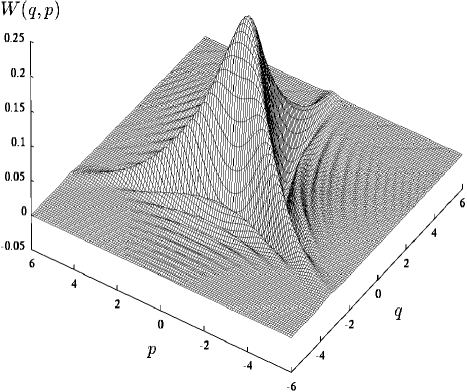
FIG. 4.: The Wigner function representing the signal field state generated using a pump with Gaussian noise, characterized by the parameters $\beta_{0}=8$ and $\bar{n}=2$. The interaction time is $t=0.025/\lambda$.

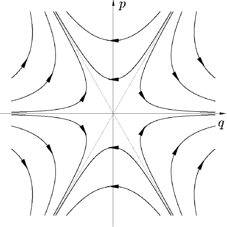
FIG. 5.: Classical trajectories of the signal mode in the approximation of a constant pump.

REFERENCES

- [1] Permanent address: Instytut Fizyki Teoretycznej, Uniwersytet Warszawski, Hoża 69, PL–00–681 Warszawa, Poland.
- [2] J. A. Wheeler, Lett. Math. Phys. 10, 201 (1985); W. P. Schleich and J. A. Wheeler, Nature 326, 574 (1987); J. Opt. Soc. Am. B 4, 1715 (1987); W. Schleich, D. F. Walls, and J. A. Wheeler, Phys. Rev. A 38, 1177 (1988); J. P. Dowling, W. P. Schleich, and J. A. Wheeler, Ann. Phys. (Leipzig) 48, 423 (1991).
- [3] K. Vogel and H. Risken, Phys. Rev. A 40, R2847 (1989).
- [4] D. T. Smithey, M. Beck, M. G. Raymer, and A. Faridani, Phys. Rev. Lett. 70, 1244 (1993); D. T. Smithey, M. Beck, J. Cooper, M. G. Raymer, and A. Faridani, Phys. Scr. T48, 35 (1993).
- [5] G. Breitenbach, T. Müller, S. F. Pereira, J.-Ph. Poizat, S. Schiller, and J. Mlynek, J. Opt. Soc. Am. B 12, 2304 (1995).
- [6] T. J. Dunn, I. A. Walmsley, and S. Mukamel, Phys. Rev. Lett. 74, 884 (1995).
- [7] D. Leibfried, D. M. Meekhof, B. E. King, C. Monroe, W. M. Itano, and D. J. Wineland, Phys. Rev. Lett. (to be published).
- [8] Ch. Kurtsiefer, T. Pfau, and J. Mlynek, presented in European Quantum Electronics Conference ’96 (unpublished); U. Janicke and M. Wilkens, J. Mod. Opt. 42, 2183 (1995); M. G. Raymer, M. Beck, and D. F. McAlister, Phys. Rev. Lett. 72, 1137 (1994).
- [9] D. M. Meekhof, C. Monroe, B. E. King, W. M. Itano, and D. J. Wineland, Phys. Rev. Lett. 76, 1796 (1996); C. Monroe, D. M. Meekhof, B. E. King, and D. J. Wineland, Science 272, 1131 (1996).
- [10] W. Schleich, M. Pernigo, and F. Le Kien, Phys. Rev. A 44, 2172 (1991); for a review see V. Bužek and P. L. Knight, in Progress in Optics XXXIV, ed. by E. Wolf (North-Holland, Amsterdam, 1995).
- [11] M. Brune et. al., submitted to Phys. Rev. Lett.
- [12] B. Yurke and D. Stoler, Phys. Rev. Lett. 57, 13 (1986); G. J. Milburn and C. A. Holmes, ibid. 56, 2237 (1986); A. Mecozzi and P. Tombesi, ibid. 58, 1055 (1987).
- [13] M. Wolinsky and H. J. Carmichael, Phys. Rev. Lett. 60, 1836 (1988).
- [14] S. Song, C. M. Caves, and B. Yurke, Phys. Rev. A 41, 5261 (1990); B. Yurke, W. Schleich, and D. F. Walls, ibid. 42, 1703 (1990).
- [15] T. Ogawa, M. Ueda, and N. Imoto, Phys. Rev. Lett. 66, 1046 (1991).
- [16] S. L. Braunstein and R. I. McLachlan, Phys. Rev. A 35, 1659 (1987).
- [17] M. Hillery, Phys. Rev. A 42, 498 (1990).
- [18] S. L. Braunstein and C. M. Caves, Phys. Rev. A 42, 4115 (1990).
- [19] G. Drobný and I. Jex, Phys. Rev. A 45, 4897 (1992).
- [20] R. Tanaś and Ts. Gantsog, Phys. Rev. A 45, 5031 (1992); I. Jex, G. Drobný, and M. Matsuoka, Opt. Comm. 94, 619 (1992).
- [21] V. Bužek and G. Drobný, Phys. Rev. A 47, 1237 (1993); G. Drobný, I. Jex, and V. Bužek, Acta Phys. Slov. 44, 155 (1994).
- [22] G. Drobny and V. Bužek, Phys. Rev. A 50, 3492 (1994).
- [23] T. Felbinger, S. Schiller, and J. Mlynek, presented in European Quantum Electronics Conference’96 (unpublished).
- [24] M. V. Berry, Philos. Trans. R. Soc. London 287, 237 (1977); E. J. Heller, J. Chem. Phys. 67, 3339 (1977); H. J. Korsch, J. Phys. A 12, 811 (1979).
- [25] U. Leonhardt and H. Paul, Phys. Rev. A 48, 4598 (1993).
- [26] E. S. Polzik, J. Carri, and H. J. Kimble, Phys. Rev. Lett. 68, 3020 (1992).
- [27] V. Bužek and P. L. Knight, Opt. Comm. 81, 331 (1991).
- [28] B. C. Sanders, Phys. Rev. A 39, 4284 (1989).
- [29] G. S. Prakash and G. S. Agarwal, Phys. Rev. A 50, 4258 (1994).
- [30] G. Drobný, A. Bandilla, and I. Jex, Phys. Rev. A (to be published).