Phase Coexistence Properties of Polarizable Stockmayer Fluids

I Abstract

We report the phase coexistence properties of polarizable Stockmayer fluids of reduced permanent dipoles $|\mathchoice{{\hbox{\boldmath$\displaystyle m$}}}{{\hbox{\boldmath$\textstyle m$}}}{{\hbox{\boldmath$\scriptstyle m$}}}{{\hbox{\boldmath$\scriptscriptstyle m$}}}_{0}^{*}|=$ 1.0 and 2.0 and reduced polarizabilities $\alpha^{*}=$ 0.00, 0.03, and 0.06, calculated by a series of grand canonical Monte Carlo simulations with the histogram reweighting method. In the histogram reweighting method, the distributions of density and energy calculated in Grand Canonical Monte Carlo simulations are stored in histograms and analyzed to construct the grand canonical partition function of the system. All thermodynamic properties are calculated from the grand partition function. The results are compared with Wertheim’s renormalization perturbation theory. Deviations between theory and simulation results for the coexistence envelope are near 2% for the lower dipole moment and 10 % for the higher dipole moment we studied.

II Introduction

Stockmayer fluids [2] have long been studied as models for fluids with permanent dipoles, such as water, ammonia, or methyl chloride. Thermodynamic properties for these fluids have been calculated by theory and simulations. Attempts have been made to model real dipolar fluids by fitting potential parameters of Stockmayer fluids. Rowlinson [3] fitted experimental second virial coefficients to theoretically calculated ones to find Stockmayer potential parameters $\epsilon$, $\sigma$, and $|\mathchoice{{\hbox{\boldmath$\displaystyle m$}}}{{\hbox{\boldmath$\textstyle m$}}}{{\hbox{\boldmath$\scriptstyle m$}}}{{\hbox{\boldmath$\scriptscriptstyle m$}}}|$ for some dipolar fluids. Van Leeuwen [4] fitted experimental coexistence curves to results from computer simulations. Agreement between the Stockmayer potential parameters calculated from second virial coefficients and phase coexistence data is only qualitative. One of the reasons why the agreement is not quantitative is that fitting of the second virial coefficient gives the parameters for the fluid at the limit of zero density while fitting of the coexistence curve gives the parameters for the dense fluid. The interaction of dipolar molecules can significantly change depending on the density or temperature due to the redistribution of electron density within a molecule in response to changes in the molecular environment (electrostatic induction effect). It is essential to account for this effect when phase coexistence properties of dipolar fluids are calculated because electrostatic induction is much stronger in the liquid phase than in the gas phase, and molecular interactions cannot be accurately modeled by the same (non-polarizable) model and parameters for both phases. One way to include the electrostatic induction effect on a model of polar fluids is to introduce polarizability.

Wertheim [5] has studied the effect of polarizability on thermodynamic properties by using a graph-theoretical approach. His renormalization perturbation theory [6] was then extended to mixtures by Venkatasubramanian et al. [7]. Patey et al. [8] performed Monte Carlo simulations to test the free energy calculation by Wertheim’s theory for hard spheres with moderately large reduced dipoles $|\mathchoice{{\hbox{\boldmath$\displaystyle m$}}}{{\hbox{\boldmath$\textstyle m$}}}{{\hbox{\boldmath$\scriptstyle m$}}}{{\hbox{\boldmath$\scriptscriptstyle m$}}}_{0}^{*}|=|\mathchoice{{\hbox{\boldmath$\displaystyle m$}}}{{\hbox{\boldmath$\textstyle m$}}}{{\hbox{\boldmath$\scriptstyle m$}}}{{\hbox{\boldmath$\scriptscriptstyle m$}}}_{0}|/\sqrt{kTd^{3}}=$ 1.0 (where $\textstyle m_{0}$ is the permanent dipole moment) and reduced mean polarizabilities of $\alpha^{*}=\alpha/d^{3}=0.03,0.06,0.1$ (where $k$ is Boltzmann constant, $T$ is the absolute temperature, $d$ is the hard sphere diameter and $\alpha$ is polarizability). Venkatasubramanian et al. compared theoretically calculated coexistence properties with experiment [7] for Stockmayer fluids with reduced dipoles of $|\mathchoice{{\hbox{\boldmath$\displaystyle m$}}}{{\hbox{\boldmath$\textstyle m$}}}{{\hbox{\boldmath$\scriptstyle m$}}}{{\hbox{\boldmath$\scriptscriptstyle m$}}}_{0}^{*}|=|\mathchoice{{\hbox{\boldmath$\displaystyle m$}}}{{\hbox{\boldmath$\textstyle m$}}}{{\hbox{\boldmath$\scriptstyle m$}}}{{\hbox{\boldmath$\scriptscriptstyle m$}}}_{0}|/\sqrt{\epsilon\sigma^{3}}\simeq 1.0$ and reduced polarizabilities of $\alpha^{*}=\alpha/\sigma^{3}\simeq 0.06$ ($\epsilon$ and $\sigma$ are the Lennard-Jones parameters). The results of these studies agree reasonably well with Wertheim’s theory. Vesely [9] performed molecular dynamics simulations of polarizable Stockmayer fluids and calculated the effect of polarizability on thermodynamic properties such as internal energy or pressure. Smit et al. [10] and van Leeuwen et al. [11] performed Gibbs ensemble Monte Carlo simulations of coexistence properties for non-polarizable Stockmayer fluids. However, simulation studies of the coexistence properties of polarizable Stockmayer fluids have not been previously published to our knowledge.

In this paper, we present results from Grand Canonical Monte Carlo (GCMC) simulations of Stockmayer fluids with and without polarizability for the vapor- liquid phase coexistence properties. The results are compared to the renormalization perturbation theory by Wertheim [6, 7]. We study the models with reduced dipoles of $|\mathchoice{{\hbox{\boldmath$\displaystyle m$}}}{{\hbox{\boldmath$\textstyle m$}}}{{\hbox{\boldmath$\scriptstyle m$}}}{{\hbox{\boldmath$\scriptscriptstyle m$}}}_{0}^{*}|=$ 1.0 and 2.0 and reduced polarizabilities of $\alpha^{*}=$0.00, 0.03, and 0.06. Examples of estimates of the parameters for real fluids are $|\mathchoice{{\hbox{\boldmath$\displaystyle m$}}}{{\hbox{\boldmath$\textstyle m$}}}{{\hbox{\boldmath$\scriptstyle m$}}}{{\hbox{\boldmath$\scriptscriptstyle m$}}}_{0}^{*}|=$ 1.84 and $\alpha^{*}=$0.08 for water [3] and $|\mathchoice{{\hbox{\boldmath$\displaystyle m$}}}{{\hbox{\boldmath$\textstyle m$}}}{{\hbox{\boldmath$\scriptstyle m$}}}{{\hbox{\boldmath$\scriptscriptstyle m$}}}_{0}^{*}|=$ 1.03 and $\alpha^{*}=$0.06 for methyl chloride [7]. Since applications of the histogram reweighting method to phase coexistence of fluids have only recently started appearing[17], we begin this paper by discussing the principle of the method and issues related to its practical application to predict phase coexistence curves at temperatures significantly below the critical point.

Deviations between theory and simulation results for the coexistence envelope are near 2% for the lower dipole moment and 10 % for the higher dipole moment studied.

III GCMC Histogram reweighting method

Determination of phase coexistence by Monte Carlo simulation requires either implicit or explicit calculation of the free energy of a system. The Gibbs ensemble method [12] is used for determination of phase equilibrium by implicitly minimizing the total free energy of the system, which is separated into two phases. Non-Boltzmann sampling methods (such as thermodynamic scaling) [13, 14] and the test particle insertion method [15] are among the methods for explicit calculation of free energy of the system. Ferrenberg and Swendsen [16] proposed the use of the distribution of energy and density calculated in grand canonical Monte Carlo (GCMC) simulations. We refer to this method as “the histogram reweighting method.” The method has rarely been applied to continuous-space fluids, with the exception of a recent study by Wilding for the Lennard-Jones fluid [17]. We chose the histogram reweighting method for this study because we found it to be computationally more efficient than the other available methods for our systems.

One of the attractive features of the histogram reweighting method is that it can be used to construct the grand canonical partition function, which in turn can be used to obtain all thermodynamic properties, including the free energy or coexistence properties. Moreover, a single simulation at a given chemical potential $\mu$ and temperature $T$ can give the thermodynamic properties at a range of $\mu^{\prime}$ and $T^{\prime}$, by virtue of the scaling properties in the variables (see section on ”Theoretical Basis” below). In calculating coexistence properties, it is not necessary to observe phase coexistence in a single GCMC simulation, since they are calculated by analyzing the grand canonical partition function constructed by combining the histograms. GCMC simulation is appropriate for calculating thermodynamic properties for a range of densities for molecular fluids, because it does not require computationally expensive volume changes. The polarizable Stockmayer potential does not scale simply with volume.

A Theoretical Basis

The basic concept behind the histogram reweighting method of Ferrenberg and Swendsen [16] for GCMC simulations is reviewed here. The grand canonical partition function of a system with chemical potential $\mu$, volume $V$, and temperature $T$ is written as

$$\Xi(\mu,V,T)=\sum_{N}\sum_{U_{N}}exp[(N\beta\mu)-\beta U_{N}]\Omega(N,V,U_{N})$$ (1)

where $\Omega(N,V,U_{N})$ is the number of microstates for number of particles $N$, volume $V$ and energy $U_{N}$; the notation $U_{N}$ emphasizes that the energy level depends on the number of particles. We define the chemical potential $\mu$ by

$$\beta\mu=ln\ z$$ (2)

where $z$ is the activity. $\beta$ is the inverse temperature ($\beta=1/kT$) , where $k$ is Boltzmann’s constant. The $\displaystyle\sum_{N}$ denotes the summation over $N$ from 0 to infinity, and $\displaystyle\sum_{U_{N}}$ denotes the summation over all energy levels for each $N$. We perform GCMC simulations by Norman and Filinov’s method [18] and store the number of observations of particular $N$ and $U_{N}$ in a two dimensional histogram $f_{\mu,V,T}(N,U_{N})$, which is related to the components of the grand canonical partition function, with a simulation-specific constant $C$, by

$$f_{\mu,V,T}(N,U_{N})\cdot C=exp[(N\beta\mu)-\beta U_{N}]\Omega(N,V,U_{N})$$ (3)

The thermodynamic average of a property $X$ is calculated by

$$<X>_{\mu,V,T}=\frac{\displaystyle\sum_{N}\sum_{U_{N}}X(N,U_{N})f_{\mu,V,T}(N,U_{N})}{\displaystyle\sum_{N}\sum_{U_{N}}f_{\mu,V,T}(N,U_{N})}.$$ (4)

Next, let us consider the grand canonical partition function for a different thermodynamic state with chemical potential $\mu^{\prime}$ and temperature $T^{\prime}$, which is written as

$$\Xi(\mu^{\prime},V,T^{\prime})=$$ (5)

$$=\sum_{N}\sum_{U_{N}}{exp[(N\beta^{\prime}\mu^{\prime})-\beta^{\prime}U_{N}]\Omega(N,V,U_{N})}$$ (6)

(7)

$$=\sum_{N}\sum_{U_{N}}exp[N(\beta^{\prime}\mu^{\prime}-\beta\mu)-(\beta^{\prime}-\beta)U_{N}]\cdot$$ (8)

$$\cdot exp[(N\beta\mu)-\beta U_{N}]\Omega(N,V,U_{N})$$ (9)

(10)

$$=\sum_{N}\sum_{U_{N}}exp[N(\beta^{\prime}\mu^{\prime}-\beta\mu)-(\beta^{\prime}-\beta)U_{N}]\cdot$$ (11)

$$\cdot f_{\mu,V,T}(N,U_{N})\cdot C$$ (12)

The thermodynamic average of a property $X$ is then

$$<X>_{\mu^{\prime},V,T^{\prime}}=$$ (13)

(14)

$$=\frac{\displaystyle\sum_{N}\sum_{U_{N}}X(N,U_{N})Wf_{\mu,V,T}(N,U_{N})}{\displaystyle\sum_{N}\sum_{U_{N}}Wf_{\mu,V,T}(N,U_{N})}$$ (15)

where $W=exp[N(\beta^{\prime}\mu^{\prime}-\beta\mu)-(\beta^{\prime}-\beta)U_{N}]$. As can be seen from these equations, once we know the components of the grand canonical partition function $f_{\mu,V,T}(N,U_{N})$ at a thermodynamic state ($\mu$, $V$, $T$), we can construct a grand canonical partition function at a different thermodynamic state ($\mu^{\prime}$, $V$, $T^{\prime}$) by reweighting each component with $exp[N(\beta^{\prime}\mu^{\prime}-\beta\mu)-(\beta^{\prime}-\beta)U_{N}]$. Then, we can calculate the thermodynamic properties at the new state ($\mu^{\prime}$, $V$, $T^{\prime}$) by averaging a thermodynamic variable with the reweighted components of the grand canonical partition function. Therefore, once we have a two dimensional histogram $f_{\mu,V,T}(N,U_{N})$ from a GCMC simulation at a state ($\mu$, $V$, $T$), any thermodynamic property at any state ($\mu^{\prime}$, $V$, $T^{\prime}$). The constant $C$, which is unknown, but can be determined as described below, is unimportant in averaging a property $X$ as in equation 13 because it cancels out in the numerator and the denominator.

B Determination of phase coexistence

In the grand canonical ensemble at a sub-critical temperature, the vapor-liquid coexistence can be determined by finding the chemical potential that gives the same pressure for both phases. We define the pressure $P$ at a thermodynamic state ($\mu$, $V$, $T$) by

$$P_{\mu,V,T}=\frac{1}{V}ln\ \Xi(\mu,V,T)$$ (16)

If a histogram is made for a thermodynamic state ($\mu$, $V$, $T$), the pressure at ($\mu^{\prime}$, $V$, $T^{\prime}$) is calculated by

$$P_{\mu^{\prime},V,T^{\prime}}=$$ (17)

$$=\frac{1}{V}ln\sum_{N}\sum_{U_{N}}exp[N(\beta^{\prime}\mu^{\prime}-\beta\mu)-(\beta^{\prime}-\beta)U_{N}]\cdot$$ (18)

$$\cdot f_{\mu,V,T}(N,U_{N})\cdot C$$ (19)

where equations 5 and 16 are used. At a subcritical temperature, the pressure of each phase is thus calculated except for the constant $C$. The chemical potential $\mu^{\prime}$ that gives the same pressure for both phases is then found, and the phase coexistence thus determined. When it is necessary to calculate the absolute value of the partition function, the simulation specific constant $C$ needs to be determined by a different means. In this study, the absolute value of the constant $C$ is fixed by calculating the pressure in the original simulation using the virial theorem

$$P=\frac{<N>_{\mu,V,T}}{V}kT+\Big{<}\frac{dU}{dV}\Big{>}_{\mu,V,T}$$ (20)

and equating that with the pressure calculated by equation 19.

C Combining Results of Several Simulations

Calculation of the thermodynamic properties at vapor-liquid coexistence requires the histogram over a wide range of $N$ and $U_{N}$. However, it is difficult to get $f_{\mu,V,T}(N,U_{N})$ with good statistical accuracy over a wide range of $N$ and $U_{N}$ from one simulation. In the method by Norman and Filinov [18] or in any Metropolis scheme [19], the configurations relevant to the given thermodynamic state ($\mu$, $V$, $T$) are preferentially sampled and those relevant to other states are not sampled well. Therefore, we perform several simulations at different thermodynamic states and combine the information to construct the histogram $f_{\mu,V,T}(N,U_{N})$, which is then given with good accuracy over a wide range of $N$ and $U_{N}$. In the initial attempts to sample a wide range of $N$ and $U_{N}$, we perform GCMC simulations at a temperature slightly above the critical point with various chemical potentials. The details are described in section 5.

Combining two simulation results is done by fixing the ratio of the simulation specific constants $C$ for two simulations at different thermodynamic states (denoted by subscripts 1 and 2) by imposing

$$\sum_{U_{N}}exp[N(\beta\mu-\beta_{1}\mu_{1})-(\beta-\beta_{1})U_{N}]\cdot$$ (21)

$$\cdot f_{\mu_{1},V,T_{1}}(N,U_{N})\cdot C_{1}$$ (22)

$$=\sum_{U_{N}}exp[N(\beta\mu-\beta_{2}\mu_{2})-(\beta-\beta_{2})U_{N}]\cdot$$ (23)

$$f_{\mu_{2},V,T_{2}}(N,U_{N})\cdot C_{2}$$ (24)

at the same $N$ and $T$: if the original simulations are performed at different temperatures, one or both histograms need to be reweighted so that the two histograms are compared at the same temperature. It is necessary to choose $N$ and $T$ for which the relevant configurations are sampled by both simulations. For convenience, we choose $T$ as the average of the temperatures for the two original simulations and $N$ as the number of particles at which the density distributions at temperature $T$ overlap most. A more sophisticated way of combining multiple simulation results, utilizing information for a range of $N$ instead of one $N$, has been proposed by Ferrenberg and Swendsen [20]. The simpler method described above was found to be satisfactory for our systems.

D Comparison to the Gibbs Ensemble method

Both the GCMC histogram reweighting method and the Gibbs ensemble method [12] can be used to obtain the coexistence properties of a system such as the polarizable Stockmayer fluid of the present study. At first sight, it would seem that the Gibbs ensemble method is simpler to implement, as it requires only a single simulation per temperature at which coexistence is to be determined, rather than the series of simulations required by the GCMC histogram method. To determine the complete phase diagram at a series of temperatures both methods require several simulations. However, we have found that statistical uncertainties for the coexistence properties from the GCMC method seem to be significantly smaller than for a Gibbs-ensemble determination of the phase behavior for comparable amounts of computational time expenditure. This statement is supported by the small statistical uncertainties of the coexistence properties calculated in Tables III and IV, which would have required prohibitively long Gibbs ensemble calculations.

IV Model

A molecule of a Stockmayer fluid is a Lennard-Jones interaction site with an embedded point dipole at the center of the molecule. For polarizable models, polarizability is introduced also at the center of the molecule [8, 9]. Assuming that the induced dipole moment is linearly dependent on the local electric field at the center of the molecule, the total dipole moment of molecule $i$ is written as

$$\mathchoice{{\hbox{\boldmath$\displaystyle m$}}}{{\hbox{\boldmath$\textstyle m$}}}{{\hbox{\boldmath$\scriptstyle m$}}}{{\hbox{\boldmath$\scriptscriptstyle m$}}}_{i}=\mathchoice{{\hbox{\boldmath$\displaystyle m$}}}{{\hbox{\boldmath$\textstyle m$}}}{{\hbox{\boldmath$\scriptstyle m$}}}{{\hbox{\boldmath$\scriptscriptstyle m$}}}_{0,i}+\mathchoice{{\hbox{\boldmath$\displaystyle\alpha$}}}{{\hbox{\boldmath$\textstyle\alpha$}}}{{\hbox{\boldmath$\scriptstyle\alpha$}}}{{\hbox{\boldmath$\scriptscriptstyle\alpha$}}}\cdot\mathchoice{{\hbox{\boldmath$\displaystyle E$}}}{{\hbox{\boldmath$\textstyle E$}}}{{\hbox{\boldmath$\scriptstyle E$}}}{{\hbox{\boldmath$\scriptscriptstyle E$}}}_{i},$$ (25)

where $\mathchoice{{\hbox{\boldmath$\displaystyle m$}}}{{\hbox{\boldmath$\textstyle m$}}}{{\hbox{\boldmath$\scriptstyle m$}}}{{\hbox{\boldmath$\scriptscriptstyle m$}}}_{i}$ is the total dipole moment, $\mathchoice{{\hbox{\boldmath$\displaystyle m$}}}{{\hbox{\boldmath$\textstyle m$}}}{{\hbox{\boldmath$\scriptstyle m$}}}{{\hbox{\boldmath$\scriptscriptstyle m$}}}_{0,i}$ is the permanent dipole moment, $\mathchoice{{\hbox{\boldmath$\displaystyle E$}}}{{\hbox{\boldmath$\textstyle E$}}}{{\hbox{\boldmath$\scriptstyle E$}}}{{\hbox{\boldmath$\scriptscriptstyle E$}}}_{i}$ is the local electric field at the center of the molecule, and $\textstyle\alpha$ is the polarizability tensor. The local electric field is calculated as [21]

$$\mathchoice{{\hbox{\boldmath$\displaystyle E$}}}{{\hbox{\boldmath$\textstyle E$}}}{{\hbox{\boldmath$\scriptstyle E$}}}{{\hbox{\boldmath$\scriptscriptstyle E$}}}_{i}=\sum_{j\neq i}\mathchoice{{\hbox{\boldmath$\displaystyle T$}}}{{\hbox{\boldmath$\textstyle T$}}}{{\hbox{\boldmath$\scriptstyle T$}}}{{\hbox{\boldmath$\scriptscriptstyle T$}}}_{ij}\cdot\mathchoice{{\hbox{\boldmath$\displaystyle m$}}}{{\hbox{\boldmath$\textstyle m$}}}{{\hbox{\boldmath$\scriptstyle m$}}}{{\hbox{\boldmath$\scriptscriptstyle m$}}}_{j},$$ (26)

where $\mathchoice{{\hbox{\boldmath$\displaystyle T$}}}{{\hbox{\boldmath$\textstyle T$}}}{{\hbox{\boldmath$\scriptstyle T$}}}{{\hbox{\boldmath$\scriptscriptstyle T$}}}_{ij}$ is the dipole tensor for molecules $i$ and $j$. If the vector connecting the centers of molecules $i$ and $j$ is written as $\mathchoice{{\hbox{\boldmath$\displaystyle r$}}}{{\hbox{\boldmath$\textstyle r$}}}{{\hbox{\boldmath$\scriptstyle r$}}}{{\hbox{\boldmath$\scriptscriptstyle r$}}}_{ij}$ and the unit tensor as $\mathchoice{{\hbox{\boldmath$\displaystyle I$}}}{{\hbox{\boldmath$\textstyle I$}}}{{\hbox{\boldmath$\scriptstyle I$}}}{{\hbox{\boldmath$\scriptscriptstyle I$}}}_{ij}$, the dipole tensor is defined as

$$\mathchoice{{\hbox{\boldmath$\displaystyle T$}}}{{\hbox{\boldmath$\textstyle T$}}}{{\hbox{\boldmath$\scriptstyle T$}}}{{\hbox{\boldmath$\scriptscriptstyle T$}}}_{ij}=\frac{3\mathchoice{{\hbox{\boldmath$\displaystyle r$}}}{{\hbox{\boldmath$\textstyle r$}}}{{\hbox{\boldmath$\scriptstyle r$}}}{{\hbox{\boldmath$\scriptscriptstyle r$}}}_{ij}\mathchoice{{\hbox{\boldmath$\displaystyle r$}}}{{\hbox{\boldmath$\textstyle r$}}}{{\hbox{\boldmath$\scriptstyle r$}}}{{\hbox{\boldmath$\scriptscriptstyle r$}}}_{ij}}{{r_{ij}}^{5}}-\frac{\mathchoice{{\hbox{\boldmath$\displaystyle I$}}}{{\hbox{\boldmath$\textstyle I$}}}{{\hbox{\boldmath$\scriptstyle I$}}}{{\hbox{\boldmath$\scriptscriptstyle I$}}}_{ij}}{{r_{ij}}^{3}}$$ (27)

where

$$r_{ij}=|\mathchoice{{\hbox{\boldmath$\displaystyle r$}}}{{\hbox{\boldmath$\textstyle r$}}}{{\hbox{\boldmath$\scriptstyle r$}}}{{\hbox{\boldmath$\scriptscriptstyle r$}}}_{ij}|$$ (28)

The total interaction of a Stockmayer fluid is $U=U_{LJ}+U_{dp}$ , where

$$U_{LJ}=\sum_{i\neq j}4\epsilon\Big{[}(\frac{\sigma}{r_{ij}})^{12}-(\frac{\sigma}{r_{ij}})^{6}\Big{]}$$ (29)

$$U_{dp}=-\frac{1}{2}\sum_{i}\mathchoice{{\hbox{\boldmath$\displaystyle m$}}}{{\hbox{\boldmath$\textstyle m$}}}{{\hbox{\boldmath$\scriptstyle m$}}}{{\hbox{\boldmath$\scriptscriptstyle m$}}}_{i}\cdot\mathchoice{{\hbox{\boldmath$\displaystyle E$}}}{{\hbox{\boldmath$\textstyle E$}}}{{\hbox{\boldmath$\scriptstyle E$}}}{{\hbox{\boldmath$\scriptscriptstyle E$}}}_{i}+\frac{1}{2}\sum_{i}\mathchoice{{\hbox{\boldmath$\displaystyle E$}}}{{\hbox{\boldmath$\textstyle E$}}}{{\hbox{\boldmath$\scriptstyle E$}}}{{\hbox{\boldmath$\scriptscriptstyle E$}}}_{i}\cdot\mathchoice{{\hbox{\boldmath$\displaystyle\alpha$}}}{{\hbox{\boldmath$\textstyle\alpha$}}}{{\hbox{\boldmath$\scriptstyle\alpha$}}}{{\hbox{\boldmath$\scriptscriptstyle\alpha$}}}\cdot\mathchoice{{\hbox{\boldmath$\displaystyle E$}}}{{\hbox{\boldmath$\textstyle E$}}}{{\hbox{\boldmath$\scriptstyle E$}}}{{\hbox{\boldmath$\scriptscriptstyle E$}}}_{i}$$ (30)

$$=-\frac{1}{2}\sum_{i}\mathchoice{{\hbox{\boldmath$\displaystyle m$}}}{{\hbox{\boldmath$\textstyle m$}}}{{\hbox{\boldmath$\scriptstyle m$}}}{{\hbox{\boldmath$\scriptscriptstyle m$}}}_{0,i}\cdot\mathchoice{{\hbox{\boldmath$\displaystyle E$}}}{{\hbox{\boldmath$\textstyle E$}}}{{\hbox{\boldmath$\scriptstyle E$}}}{{\hbox{\boldmath$\scriptscriptstyle E$}}}_{i}$$ (31)

In these equations, $U_{LJ}$ and $U_{dp}$ denote the Lennard-Jones interaction and the dipole-dipole interaction, respectively. $\epsilon$ and $\sigma$ are the Lennard-Jones parameters. Since the total dipole mement of each molecule depends on the dipole moments of other molecules, the energy is calculated by an iterative procedure. Details of the iterative procedure are discussed in the next section.

V Simulation Details

Throughout this study, data are presented in the reduced units, denoted by the superscript (*). The units of energy and length are reduced by the Lennard-Jones parameters $\epsilon$ and $\sigma$, respectively. Reduced temperature is $T^{*}=kT/\epsilon$. Dipole moment ($\textstyle m$) and polarizability ($\textstyle\alpha$) are reduced by the Lennard-Jones parameters as $\displaystyle\mathchoice{{\hbox{\boldmath$\displaystyle m$}}}{{\hbox{\boldmath$\textstyle m$}}}{{\hbox{\boldmath$\scriptstyle m$}}}{{\hbox{\boldmath$\scriptscriptstyle m$}}}^{*}=\mathchoice{{\hbox{\boldmath$\displaystyle m$}}}{{\hbox{\boldmath$\textstyle m$}}}{{\hbox{\boldmath$\scriptstyle m$}}}{{\hbox{\boldmath$\scriptscriptstyle m$}}}/\sqrt{\epsilon\sigma^{3}}$ and $\mathchoice{{\hbox{\boldmath$\displaystyle\alpha$}}}{{\hbox{\boldmath$\textstyle\alpha$}}}{{\hbox{\boldmath$\scriptstyle\alpha$}}}{{\hbox{\boldmath$\scriptscriptstyle\alpha$}}}^{*}=\mathchoice{{\hbox{\boldmath$\displaystyle\alpha$}}}{{\hbox{\boldmath$\textstyle\alpha$}}}{{\hbox{\boldmath$\scriptstyle\alpha$}}}{{\hbox{\boldmath$\scriptscriptstyle\alpha$}}}/\sigma^{3}$. We study Stockmayer fluids with permanent dipole moments $|\mathchoice{{\hbox{\boldmath$\displaystyle m_{0}$}}}{{\hbox{\boldmath$\textstyle m_{0}$}}}{{\hbox{\boldmath$\scriptstyle m_{0}$}}}{{\hbox{\boldmath$\scriptscriptstyle m_{0}$}}}^{*}|=$ 1.0 and 2.0 and isotropic polarizabilities $\alpha^{*}=$ 0.00, 0.03, and 0.06.

In GCMC simulations, at each Monte Carlo step, a new microstate is generated by a displacement, rotation, and creation or destruction of a molecule. The state thus generated is probabilistically accepted so that the limiting distribution of generated microstates obeys the grand canonical ensemble. We use 10% of the Monte Carlo moves for displacement, 10% for rotation, 40% for creation, and 40% for destruction. In the energy calculation of polarizable models, the total interaction of the system is calculated by an iterative procedure [8, 9, 22] described below.

The initial values of properties for a configuration are indicated by (0), and the estimates for those properties at the k-th iteration by (k). When a molecule is either displaced, rotated, created or destroyed, the initial estimate of the electric field at the center of molecule $i$ is

$$\mathchoice{{\hbox{\boldmath$\displaystyle E$}}}{{\hbox{\boldmath$\textstyle E$}}}{{\hbox{\boldmath$\scriptstyle E$}}}{{\hbox{\boldmath$\scriptscriptstyle E$}}}_{i}(1)=\sum_{j\neq i}\mathchoice{{\hbox{\boldmath$\displaystyle T$}}}{{\hbox{\boldmath$\textstyle T$}}}{{\hbox{\boldmath$\scriptstyle T$}}}{{\hbox{\boldmath$\scriptscriptstyle T$}}}_{ij}\cdot\mathchoice{{\hbox{\boldmath$\displaystyle m$}}}{{\hbox{\boldmath$\textstyle m$}}}{{\hbox{\boldmath$\scriptstyle m$}}}{{\hbox{\boldmath$\scriptscriptstyle m$}}}_{j}(0)$$ (32)

Then, the first estimate of the total dipole mement of molecule i is

$$\mathchoice{{\hbox{\boldmath$\displaystyle m$}}}{{\hbox{\boldmath$\textstyle m$}}}{{\hbox{\boldmath$\scriptstyle m$}}}{{\hbox{\boldmath$\scriptscriptstyle m$}}}_{i}(1)=\mathchoice{{\hbox{\boldmath$\displaystyle m$}}}{{\hbox{\boldmath$\textstyle m$}}}{{\hbox{\boldmath$\scriptstyle m$}}}{{\hbox{\boldmath$\scriptscriptstyle m$}}}_{0,i}+\mathchoice{{\hbox{\boldmath$\displaystyle\alpha$}}}{{\hbox{\boldmath$\textstyle\alpha$}}}{{\hbox{\boldmath$\scriptstyle\alpha$}}}{{\hbox{\boldmath$\scriptscriptstyle\alpha$}}}\cdot\mathchoice{{\hbox{\boldmath$\displaystyle E$}}}{{\hbox{\boldmath$\textstyle E$}}}{{\hbox{\boldmath$\scriptstyle E$}}}{{\hbox{\boldmath$\scriptscriptstyle E$}}}_{i}(1),$$ (33)

and the total electrostatic interaction is

$$U_{dp}(1)=-\frac{1}{2}\sum_{i}\mathchoice{{\hbox{\boldmath$\displaystyle m$}}}{{\hbox{\boldmath$\textstyle m$}}}{{\hbox{\boldmath$\scriptstyle m$}}}{{\hbox{\boldmath$\scriptscriptstyle m$}}}_{0,i}\cdot\mathchoice{{\hbox{\boldmath$\displaystyle E$}}}{{\hbox{\boldmath$\textstyle E$}}}{{\hbox{\boldmath$\scriptstyle E$}}}{{\hbox{\boldmath$\scriptscriptstyle E$}}}_{i}(1).$$ (34)

This way, the k-th estimates of the electric field, the dipole mement, and the dipole-dipole interaction are

$$\mathchoice{{\hbox{\boldmath$\displaystyle E$}}}{{\hbox{\boldmath$\textstyle E$}}}{{\hbox{\boldmath$\scriptstyle E$}}}{{\hbox{\boldmath$\scriptscriptstyle E$}}}_{i}(k)=\sum_{j\neq i}\mathchoice{{\hbox{\boldmath$\displaystyle T$}}}{{\hbox{\boldmath$\textstyle T$}}}{{\hbox{\boldmath$\scriptstyle T$}}}{{\hbox{\boldmath$\scriptscriptstyle T$}}}_{ij}\cdot\mathchoice{{\hbox{\boldmath$\displaystyle m$}}}{{\hbox{\boldmath$\textstyle m$}}}{{\hbox{\boldmath$\scriptstyle m$}}}{{\hbox{\boldmath$\scriptscriptstyle m$}}}_{j}(k-1)$$ (35)

$$\mathchoice{{\hbox{\boldmath$\displaystyle m$}}}{{\hbox{\boldmath$\textstyle m$}}}{{\hbox{\boldmath$\scriptstyle m$}}}{{\hbox{\boldmath$\scriptscriptstyle m$}}}_{i}(k)=\mathchoice{{\hbox{\boldmath$\displaystyle m$}}}{{\hbox{\boldmath$\textstyle m$}}}{{\hbox{\boldmath$\scriptstyle m$}}}{{\hbox{\boldmath$\scriptscriptstyle m$}}}_{0,i}+\mathchoice{{\hbox{\boldmath$\displaystyle\alpha$}}}{{\hbox{\boldmath$\textstyle\alpha$}}}{{\hbox{\boldmath$\scriptstyle\alpha$}}}{{\hbox{\boldmath$\scriptscriptstyle\alpha$}}}\cdot\mathchoice{{\hbox{\boldmath$\displaystyle E$}}}{{\hbox{\boldmath$\textstyle E$}}}{{\hbox{\boldmath$\scriptstyle E$}}}{{\hbox{\boldmath$\scriptscriptstyle E$}}}_{i}(k),$$ (36)

$$U_{dp}(k)=-\frac{1}{2}\sum_{i}\mathchoice{{\hbox{\boldmath$\displaystyle m$}}}{{\hbox{\boldmath$\textstyle m$}}}{{\hbox{\boldmath$\scriptstyle m$}}}{{\hbox{\boldmath$\scriptscriptstyle m$}}}_{0,i}\cdot\mathchoice{{\hbox{\boldmath$\displaystyle E$}}}{{\hbox{\boldmath$\textstyle E$}}}{{\hbox{\boldmath$\scriptstyle E$}}}{{\hbox{\boldmath$\scriptscriptstyle E$}}}_{i}(k)$$ (37)

respectively. This procedure is repeated until $U_{dp}(k)$ is converged so that $|U_{dp}(k)-U_{dp}(k-1)|/|U_{dp}(k-1)|<0.0001$ for two consecutive iterations. Typically, the number of iterations required for this criterion at each Monte Carlo move turns out to be 3 to 4 for polarizability of $\alpha^{*}=$ 0.03 and 3 to 6 for $\alpha^{*}=$ 0.06 (see tables 1 and 2). The initial value of dipole moment of molecule $i(\mathchoice{{\hbox{\boldmath$\displaystyle m$}}}{{\hbox{\boldmath$\textstyle m$}}}{{\hbox{\boldmath$\scriptstyle m$}}}{{\hbox{\boldmath$\scriptscriptstyle m$}}}_{i}(0))$ at each Monte Carlo step is chosen to be the dipole moment before the move, except for a newly inserted molecule for which the dipole moment is chosen to be the same as the permanent dipole moment. The dipole points to a random direction for a newly inserted molecule. In order to minimize the size effect for the dipole-dipole interaction, we use the Ewald sum with 256 vectors for the reciprocal space terms [23] for the model with $|\mathchoice{{\hbox{\boldmath$\displaystyle m_{0}$}}}{{\hbox{\boldmath$\textstyle m_{0}$}}}{{\hbox{\boldmath$\scriptstyle m_{0}$}}}{{\hbox{\boldmath$\scriptscriptstyle m_{0}$}}}^{*}|=$ 1.0 and $\alpha^{*}=$ 0.00, and 514 vectors for the other models that we study. Approximate overall cpu-time per Monte Carlo step for the polarizable models is 2 times slower for $\alpha^{*}=$ 0.03 and 2.4 times slower for $\alpha^{*}=$ 0.06 than the cpu-time for $\alpha^{*}=$ 0.00 by our code designed for polarizable models with the Ewald sum. Simulations of non-polarizable models by our code for polarizable models are, in turn, approximately 4 times slower than those by our code specifically designed for non-polarizable models, because the energy calculation of polarizable models requires the calculation of the local electric field of each molecule.

When two polarizable molecules approach unphysically close to each other during simulation, the electrostatic attraction increases faster than the repulsive part of the Lennard-Jones potential due to the increasing magnitude of the total dipoles and eventually the two molecules overlap [22]. In order to avoid this effect, we set a saturation point of the total dipole equal to twice the magnitude of the permanent dipole. This treatment seems to be reasonable because the average of the total dipole moment is far smaller than twice the magnitude of the permanent dipole in each of the simulations we performed (see tables 1 and 2). For the Lennard-Jones interaction, the potential is cut off at half of the simulation box length and the standard long range correction is applied [24].

During the simulations, the number of observations of a given number of particles and energy is counted and the two dimensional histogram $f_{\mu,V,T}(N,U_{N})$ is made. The grid of the histogram for energy is chosen to be 0.01 in the reduced unit. The two dimensional histograms of the number of particles and the energy are analyzed to obtain coexistence properties for a range of temperature by the method described in section 2.

In most simulations, the volume is chosen to be $V^{*}$=216. For simulations of low densities, the volume is chosen to be $V^{*}$=2160 so that the simulation box can accommodate a large enough number of particles to measure a density difference as small as $\Delta\rho^{*}=\Delta[1/V^{*}]\simeq$ 0.0005. In combining the histograms of simulations of different volumes, we rescale the histogram for $V^{*}$=2160 to that for $V^{*}$=216 assuming

$$\Omega(N,V,T)={\Omega(kN,kV,T)}^{\frac{1}{k}},$$ (38)

or, in terms of the component of the histogram,

$$f_{\mu,V,T}(N,U_{N})={f_{\mu,kV,T}(kN,U_{kN})}^{\frac{1}{k}}$$ (39)

which is a reasonable assumption away from the critical point, since the logarithms of the microcanonical and canonical partition functions are extensive properties of the system.

To fix the simulation specific constant $C$, we use the pressure calculated by the virial theorem in one of the simulations in the gas phase. The derivative of energy in terms of volume is calculated by an approximation,

$$\frac{dU}{dV}\simeq\frac{U(V+\delta V)-U(V)}{\delta V}.$$ (40)

The $\delta V$ is chosen to be about 3% of the volume $V$. The energy $U(V+\delta V)$ is calculated every time a Monte Carlo move is accepted.

For each model, we first estimate the approximate location of the critical point by looking up literature values for similar models [10, 11] and by performing several short test simulations. Then, we perform a series of GCMC simulations at a temperature slightly above the critical temperature for various chemical potentials to sample a wide range of density. The reasons why we choose a temperature slightly above the critical temperature are that large density fluctuations near the critical point make it easier to sample a wide range of density in a single simulation and that for subcritical temperatures the system tends to fluctuate infrequently between the gas and liquid densities, making sampling of both phases difficult.

An example is illustrated in figure 1 for the model with $|\mathchoice{{\hbox{\boldmath$\displaystyle m_{0}$}}}{{\hbox{\boldmath$\textstyle m_{0}$}}}{{\hbox{\boldmath$\scriptstyle m_{0}$}}}{{\hbox{\boldmath$\scriptscriptstyle m_{0}$}}}^{*}|=1.0$ and $\alpha^{*}=0.03$. At $T^{*}$=1.5, we performed GCMC simulations with various chemical potentials ($\mu^{*}=-7.00\sim-1.00$) to cover the density range of interest. The mean densities calculated from these simulations are shown in figure 1 by circles. The coexistence properties for a range of temperatures ($T^{*}=1.0\sim 1.5$ for this example) are calculated from these simulation results.

In order to make sure that the simulations are sampling the configurations relevant to the phase equilibrium properties, we performed a new series of simulations with temperatures and chemical potentials that are near the corresponding properties at phase coexistence for temperatures lower than the temperature for the first simulations ($T^{*}$=1.0, 1.1, 1.2, and 1.3). The chemical potentials for these simulations are chosen to be the values at coexistence estimated from the first simulation results for each temperature. The mean densities calculated from the new series of GCMC simulations are shown in figure 1 by squares.

The histograms obtained from the new series of simulations (below the critical point) and four of the first simulations (near the critical point) were analyzed to calculate the phase coexistence properties. The distributions of density from the histograms used for analysis are shown in figure 2 and the conditions of the simulations are listed in table 1. The fitting of the calculated coexistence densities to the law of rectilinear diameters and a scaling law, assuming that dipolar fluids obey the Ising exponent ($\beta=0.326$), is shown in figure 1 by dashed line. We performed five sets of simulations and analyses. The length of each GCMC simulation was 1 million Monte Carlo steps. The averages and the error-bars were calculated from the five sets of data. For error-bars, we use the square root of the variance of mean. Thus calculated error-bars are not, in a strict sense, statistical errors because there are several sources of statistical errors that propagate to the final results: for example, the thermodynamic states of interest here are not sampled an exactly equal number of times in the simulations. However, they are still good estimates of the reliability of the simulations and the data analysis.

As we can see in figure 1, the mean densities of the second series of simulations (squares) agree well with the final results (dashed line). Since the chemical potentials in the second series of simulations are based on the estimates from the first simulations (circles), it turns out that the estimates of coexistence densities from the first simulations are fairly accurate, considering that all the simulations were performed at one temperature ($T^{*}=1.5$).

VI Results

The magnitude of the average total dipole moment and the number of iterations necessary for the convergence of the energy calculation, with the criterion given in the previous section, are listed for polarizable models along with the conditions used for the original GCMC simulations in tables 1 and 2. The number of iterations necessary for energy calculation turns out to be 3 to 6, depending on the models and the thermodynamic states. The calculated magnitude of the induced dipole is larger for the models with larger permanent dipoles and larger polarizabilities. For the model with $|\mathchoice{{\hbox{\boldmath$\displaystyle m_{0}$}}}{{\hbox{\boldmath$\textstyle m_{0}$}}}{{\hbox{\boldmath$\scriptstyle m_{0}$}}}{{\hbox{\boldmath$\scriptscriptstyle m_{0}$}}}^{*}|=2.0$ and $\alpha^{*}=0.06$, the induced dipole is as large as 30 % of the permanent dipole at $T^{*}=1.0$ and $\rho^{*}\simeq 0.8$.

Examples of the probability density distributions from the GCMC simulations are shown in figure 2 for the Stockmayer fluid with $|\mathchoice{{\hbox{\boldmath$\displaystyle m_{0}$}}}{{\hbox{\boldmath$\textstyle m_{0}$}}}{{\hbox{\boldmath$\scriptstyle m_{0}$}}}{{\hbox{\boldmath$\scriptscriptstyle m_{0}$}}}^{*}|=1.0$ and $\alpha^{*}=0.03$. By reweighting and combining the histograms obtained from the simulations, we get the density distribution for any temperature and chemical potential. Examples of the density distributions at coexistence are shown in figure 3 for the Stockmayer fluid with $|\mathchoice{{\hbox{\boldmath$\displaystyle m_{0}$}}}{{\hbox{\boldmath$\textstyle m_{0}$}}}{{\hbox{\boldmath$\scriptstyle m_{0}$}}}{{\hbox{\boldmath$\scriptscriptstyle m_{0}$}}}^{*}|=1.0$ and $\alpha^{*}=0.03$. Because of the small system size of the simulations, the two peaks in the density distribution at coexistence overlap far below the critical temperature. We calculate the coexistence properties up to the temperature where the two peaks start to overlap. The results are shown in figures 4 to 9, and tables 3, 4 and 5. The critical temperature increases for the models of higher dipole moment and higher polarizability. The heat of vaporization is calculated from the results of internal energy, pressure, and density at coexistence.

We estimate the approximate values of the infinite-system critical temperature and density by fitting the simulation results to the law of rectilinear diameters and a scaling law, assuming that dipolar fluids obey the Ising exponent ($\beta=0.326$). Finite-size scaling methods[17] can be used to locate the critical point with a much higher accuracy than the present study, but require a series of simulations for different system sizes. The critical temperature increases as the polarizability increases for both dipoles ($|\mathchoice{{\hbox{\boldmath$\displaystyle m_{0}$}}}{{\hbox{\boldmath$\textstyle m_{0}$}}}{{\hbox{\boldmath$\scriptstyle m_{0}$}}}{{\hbox{\boldmath$\scriptscriptstyle m_{0}$}}}^{*}|=1.0$ and $2.0$) that we studied (see table 5). The effect of polarizability on the critical density is not pronounced. Our results seem to indicate a slight increase in the critical density at higher polarizabilities, but the differences are comparable to the statistical uncertainties of the calculations.

The calculated coexistence density, pressure, and heat of vaporization are compared with the renormalization perturbation theory by Wertheim figures 4 to 9. For the theoretical calculation, we follow the prescription given by Venkatasubramanian et al. [7] and use the equation of state by Johnson et al. [25] and the coefficients of the pair and triplet correlation functions calculated by Flytzani-Stephanopoulos et al. [26] and Gubbins and Twu [27] for the Lennard-Jones reference fluid. The agreement between simulation and theory is relatively good for $|\mathchoice{{\hbox{\boldmath$\displaystyle m_{0}^{*}$}}}{{\hbox{\boldmath$\textstyle m_{0}^{*}$}}}{{\hbox{\boldmath$\scriptstyle m_{0}^{*}$}}}{{\hbox{\boldmath$\scriptscriptstyle m_{0}^{*}$}}}|=1.0$, but poor for $|\mathchoice{{\hbox{\boldmath$\displaystyle m_{0}^{*}$}}}{{\hbox{\boldmath$\textstyle m_{0}^{*}$}}}{{\hbox{\boldmath$\scriptstyle m_{0}^{*}$}}}{{\hbox{\boldmath$\scriptscriptstyle m_{0}^{*}$}}}|=2.0$. Statistical uncertainties of the results are quite small, confirming the computational advantages of the histogram reweighting method.

VII Conclusions

We have calculated the phase coexistence properties of polarizable and non-polarizable Stockmayer fluids by the GCMC histogram reweighting method. In the histogram reweighting method, the grand canonical partition function of the system is constructed, from which any thermodynamic property can be derived by statistical thermodynamic analysis. Since the thermodynamic state for the grand canonical partition function can be continuously changed by “reweighting” the histograms, thermodynamic properties at thermodynamic states that are different from the thermodynamic state of the original simulation can be calculated. The statistical uncertainties of the calculated results are small, confirming the computational advantages of the histogram reweighting method over existing methods (such as Gibbs ensemble Monte Carlo[12]).

Our results for the coexistence properties were compared to Wertheim’s renormalization perturbation theory. Differences between theoretical and simulation results are within 2 % for the smaller dipole ($|\mathchoice{{\hbox{\boldmath$\displaystyle m_{0}^{*}$}}}{{\hbox{\boldmath$\textstyle m_{0}^{*}$}}}{{\hbox{\boldmath$\scriptstyle m_{0}^{*}$}}}{{\hbox{\boldmath$\scriptscriptstyle m_{0}^{*}$}}}|=1.0$) but only within 10 % for the higher dipole ($|\mathchoice{{\hbox{\boldmath$\displaystyle m_{0}^{*}$}}}{{\hbox{\boldmath$\textstyle m_{0}^{*}$}}}{{\hbox{\boldmath$\scriptstyle m_{0}^{*}$}}}{{\hbox{\boldmath$\scriptscriptstyle m_{0}^{*}$}}}|=2.0$) that we studied.

VIII Acknowledgments

The authors would like to thank Mr. Gerassimos Orkoulas for bringing the histogram reweighting method to their attention and Dr. Thomas Kraska for helpful discussions on Wertheim’s theory. Financial support for this work was provided by the Department of Energy, Office of Basic Energy Science. Supercomputing time was provided by the Cornell Theory Center.

TABLE I.: Conditions for the GCMC simulations (temperature $T^{*}$, chemical potenitial $\mu^{*}$, and volume $V^{*}$) for polarizable Stockmayer fluids with $|\mathchoice{{\hbox{\boldmath$\displaystyle m_{0}^{*}$}}}{{\hbox{\boldmath$\textstyle m_{0}^{*}$}}}{{\hbox{\boldmath$\scriptstyle m_{0}^{*}$}}}{{\hbox{\boldmath$\scriptscriptstyle m_{0}^{*}$}}}|=1.0$ and different polarizabilities ($\alpha^{*}$). The calculated average density ($\rho^{*}$) , average magnitude of the total dipole ($|\mathchoice{{\hbox{\boldmath$\displaystyle m$}}}{{\hbox{\boldmath$\textstyle m$}}}{{\hbox{\boldmath$\scriptstyle m$}}}{{\hbox{\boldmath$\scriptscriptstyle m$}}}^{*}|$) and the average number of iterations ($k_{itr}$) necessary for calculation of the energy for polarizable models at each Monte Carlo step (see text) are also listed. The numbers in parentheses are statistical uncertanties, in units of the last decimal point listed.

$\alpha^{*}$	$T^{*}$	$\mu^{*}$	$V^{*}$	$\rho^{*}$	$|\mathchoice{{\hbox{\boldmath$\displaystyle m$}}}{{\hbox{\boldmath$\textstyle m$}}}{{\hbox{\boldmath$\scriptstyle m$}}}{{\hbox{\boldmath$\scriptscriptstyle m$}}}^{*}|$	$k_{itr}$
0.03	1.00	-4.60	2160	0.0118(000)	1.0023(00)	3.2
	1.10	-4.43	2160	0.0231(001)	1.0039(01)	3.3
	1.20	-4.30	216	0.0410(001)	1.0051(00)	3.8
	1.30	-4.17	216	0.0732(007)	1.0084(01)	3.8
	1.50	-4.20	216	0.1246(018)	1.0118(02)	4.0
	1.50	-4.00	216	0.2248(087)	1.0199(07)	4.0
	1.50	-3.90	216	0.4118(118)	1.0335(08)	4.1
	1.50	-3.72	216	0.5225(068)	1.0410(07)	4.1
	1.30	-4.07	216	0.6000(060)	1.0507(06)	4.0
	1.20	-4.20	216	0.6679(030)	1.0572(04)	4.0
	1.10	-4.33	216	0.7306(055)	1.0646(08)	4.0
	1.00	-4.50	216	0.7674(024)	1.0699(05)	4.0
0.06	1.00	-4.70	2160	0.0106(000)	1.0048(01)	3.4
	1.10	-4.53	2160	0.0209(001)	1.0086(01)	3.6
	1.20	-4.40	216	0.0370(002)	1.0109(02)	4.5
	1.30	-4.17	216	0.0806(004)	1.0224(02)	4.6
	1.50	-4.10	216	0.2920(268)	1.0607(48)	5.2
	1.50	-4.085	216	0.3074(282)	1.0638(55)	5.2
	1.40	-4.03	216	0.6005(052)	1.1213(17)	5.7
	1.30	-4.07	216	0.6666(047)	1.1364(15)	5.7
	1.20	-4.20	216	0.7217(043)	1.1530(16)	5.7
	1.10	-4.33	216	0.7819(046)	1.1714(14)	5.7
	1.00	-4.50	216	0.8057(061)	1.1844(24)	5.7

TABLE II.: Conditions for the GCMC simulations with the calculated average density, average magnitude of the total dipole and the number of iteration necessary for calculation of energy for polarizable Stockmayer fluids with $|\mathchoice{{\hbox{\boldmath$\displaystyle m_{0}$}}}{{\hbox{\boldmath$\textstyle m_{0}$}}}{{\hbox{\boldmath$\scriptstyle m_{0}$}}}{{\hbox{\boldmath$\scriptscriptstyle m_{0}$}}}^{*}|=2.0$ and different polarizabilities. Notation is the same as for Table 1.

$\alpha^{*}$	$T^{*}$	$\mu^{*}$	$V^{*}$	$\rho^{*}$	$|\mathchoice{{\hbox{\boldmath$\displaystyle m$}}}{{\hbox{\boldmath$\textstyle m$}}}{{\hbox{\boldmath$\scriptstyle m$}}}{{\hbox{\boldmath$\scriptscriptstyle m$}}}^{*}|$	$k_{itr}$
0.03	1.70	-7.90	2160	0.0129(001)	2.0177(004)	3.2
	1.80	-7.70	2160	0.0211(002)	2.0264(008)	3.2
	1.90	-7.52	2160	0.0327(004)	2.0340(010)	3.2
	2.00	-7.37	216	0.0497(010)	2.0368(011)	3.7
	2.10	-7.24	216	0.0813(036)	2.0513(019)	3.6
	2.20	-7.16	216	0.1305(180)	2.0669(047)	3.7
	2.40	-7.00	216	0.2128(130)	2.0897(037)	3.7
	2.40	-6.75	216	0.3724(158)	2.1275(041)	3.7
	2.20	-6.96	216	0.5143(096)	2.1641(022)	3.8
	2.10	-7.14	216	0.5723(107)	2.1793(025)	3.8
	2.00	-7.27	216	0.6289(090)	2.1918(020)	3.8
	1.90	-7.42	216	0.6787(037)	2.2046(010)	3.8
	1.80	-7.60	216	0.7147(071)	2.2158(019)	3.8
	1.70	-7.80	216	0.7540(059)	2.2255(012)	3.8
0.06	2.00	-8.71	2160	0.0176(002)	2.0443(016)	3.4
	2.10	-8.51	2160	0.0260(001)	2.0579(007)	3.4
	2.20	-8.32	2160	0.0376(003)	2.0766(018)	3.5
	2.30	-8.14	216	0.0555(012)	2.0869(030)	4.4
	2.40	-7.98	216	0.0900(109)	2.1219(114)	4.5
	2.50	-7.85	216	0.1378(136)	2.1719(149)	4.6
	2.70	-7.60	216	0.2940(184)	2.2762(121)	4.8
	2.70	-7.40	216	0.4318(182)	2.3574(124)	5.0
	2.50	-7.70	216	0.5335(080)	2.4353(063)	5.1
	2.40	-7.83	216	0.5889(059)	2.4725(046)	5.1
	2.30	-8.04	216	0.6564(109)	2.5199(068)	5.2
	2.20	-8.22	216	0.6927(068)	2.5417(044)	5.2
	2.10	-8.41	216	0.7284(109)	2.5724(076)	5.2
	2.00	-8.61	216	0.7652(084)	2.6034(066)	5.2

TABLE III.: Calculated coexistence properties: chemical potential ($\mu^{*}$), pressure ($p^{*}$), gas phase density ($\rho^{*}_{g}$), liquid phase density ($\rho^{*}_{l}$), internal energies per molecule of gas phase ($u^{*}_{g}$) and of liquid phase ($u^{*}_{l}$), heat of vaporization per molecule ($\Delta h^{*}$) at different temperatures ($T^{*}$) for polarizable Stockmayer fluids with $|\mathchoice{{\hbox{\boldmath$\displaystyle m_{0}$}}}{{\hbox{\boldmath$\textstyle m_{0}$}}}{{\hbox{\boldmath$\scriptstyle m_{0}$}}}{{\hbox{\boldmath$\scriptscriptstyle m_{0}$}}}^{*}|=1.0$ and $\alpha^{*}=$ 0.00, 0.03, and 0.06. The numbers in parentheses are statistical uncertanties, in units of the last decimal point listed.

$\alpha^{*}$	$T^{*}$	$\mu^{*}$	$p^{*}$	$\rho^{*}_{g}$	$\rho^{*}_{l}$	$u^{*}_{g}$	$u^{*}_{l}$	$\Delta h^{*}$
0.00	1.00	-4.409(4)	.0179(1)	.0195(02)	.754(3)	-.276(05)	-6.11(3)	6.72(3)
	1.05	-4.320(3)	.0253(1)	.0258(02)	.732(2)	-.338(04)	-5.88(2)	6.49(2)
	1.10	-4.240(3)	.0345(1)	.0343(02)	.708(1)	-.407(03)	-5.65(1)	6.20(2)
	1.15	-4.167(2)	.0456(1)	.0451(02)	.682(2)	-.480(03)	-5.41(2)	5.87(2)
	1.20	-4.102(2)	.0590(1)	.0587(01)	.648(2)	-.568(02)	-5.11(2)	5.45(2)
	1.25	-4.045(2)	.0748(1)	.0766(01)	.612(2)	-.696(01)	-4.79(1)	4.95(1)
	1.30	-3.994(2)	.0934(1)	.1017(03)	.570(1)	-.891(02)	-4.44(1)	4.30(1)
0.03	1.00	-4.565(2)	.0138(1)	.0162(01)	.772(1)	-.259(02)	-6.41(1)	6.99(1)
	1.05	-4.470(3)	.0203(1)	.0219(01)	.751(3)	-.304(03)	-6.19(2)	6.79(2)
	1.10	-4.384(3)	.0284(1)	.0291(01)	.729(2)	-.349(03)	-5.96(2)	6.55(2)
	1.15	-4.306(4)	.0384(1)	.0381(02)	.700(1)	-.400(03)	-5.68(1)	6.24(1)
	1.20	-4.237(3)	.0503(2)	.0497(02)	.668(3)	-.477(03)	-5.39(2)	5.85(2)
	1.25	-4.176(3)	.0645(2)	.0650(03)	.636(3)	-.596(03)	-5.10(2)	5.40(2)
	1.30	-4.121(3)	.0813(2)	.0857(04)	.601(3)	-.770(03)	-4.80(2)	4.84(3)
	1.35	-4.072(2)	.1011(2)	.1150(05)	.556(2)	-1.016(04)	-4.42(2)	4.10(2)
0.06	1.00	-4.773(3)	.0105(1)	.0135(00)	.797(4)	-.241(04)	-6.83(3)	7.35(3)
	1.05	-4.669(3)	.0162(1)	.0182(01)	.777(2)	-.281(05)	-6.61(2)	7.19(2)
	1.10	-4.574(2)	.0233(1)	.0241(01)	.755(3)	-.320(05)	-6.37(2)	6.98(3)
	1.15	-4.487(2)	.0320(1)	.0315(01)	.729(2)	-.358(05)	-6.11(1)	6.73(2)
	1.20	-4.410(2)	.0426(2)	.0408(01)	.701(1)	-.411(03)	-5.83(1)	6.41(1)
	1.25	-4.341(2)	.0551(2)	.0528(01)	.668(2)	-.498(01)	-5.52(2)	5.99(2)
	1.30	-4.279(3)	.0699(3)	.0688(04)	.636(2)	-.634(03)	-5.23(2)	5.50(2)
	1.35	-4.224(4)	.0874(4)	.0908(09)	.602(2)	-.828(09)	-4.92(1)	4.91(2)
	1.40	-4.174(4)	.1081(6)	.1218(23)	.555(4)	-1.097(22)	-4.52(3)	4.11(4)

TABLE IV.: Calculated coexistence properties for polarizable Stockmayer fluids with $|\mathchoice{{\hbox{\boldmath$\displaystyle m_{0}$}}}{{\hbox{\boldmath$\textstyle m_{0}$}}}{{\hbox{\boldmath$\scriptstyle m_{0}$}}}{{\hbox{\boldmath$\scriptscriptstyle m_{0}$}}}^{*}|=2.0$ and $\alpha^{*}=$ 0.00, 0.03, and 0.06. Notation is the same as in table 3.

$\alpha^{*}$	$T^{*}$	$\mu^{*}$	$p^{*}$	$\rho^{*}_{g}$	$\rho^{*}_{l}$	$u^{*}_{g}$	$u^{*}_{l}$	$\Delta h^{*}$
0.00	1.60	-7.177(3)	.0224(0)	.0222(01)	.726(2)	-1.16(1)	-10.16(2)	9.97(2)
	1.65	-7.078(4)	.0300(1)	.0273(02)	.706(2)	-1.28(1)	-9.89(3)	9.67(3)
	1.70	-6.986(4)	.0388(1)	.0335(02)	.682(2)	-1.40(1)	-9.58(3)	9.28(4)
	1.75	-6.900(4)	.0490(1)	.0411(03)	.654(2)	-1.53(1)	-9.22(3)	8.82(3)
	1.80	-6.822(4)	.0607(2)	.0507(04)	.626(2)	-1.67(1)	-8.87(2)	8.30(3)
	1.85	-6.750(4)	.0741(3)	.0634(05)	.599(2)	-1.86(1)	-8.53(2)	7.72(3)
	1.90	-6.683(4)	.0896(3)	.0811(07)	.569(4)	-2.13(2)	-8.17(4)	6.98(4)
0.03	1.70	-7.893(6)	.0233(4)	.0183(01)	.758(4)	-1.11(1)	-11.48(6)	11.62(9)
	1.75	-7.783(4)	.0301(4)	.0222(01)	.741(5)	-1.22(1)	-11.21(6)	11.30(8)
	1.80	-7.679(3)	.0379(4)	.0270(01)	.720(6)	-1.34(1)	-10.91(7)	10.91(8)
	1.85	-7.582(2)	.0469(4)	.0327(00)	.697(5)	-1.46(1)	-10.58(6)	10.48(8)
	1.90	-7.492(3)	.0572(5)	.0396(00)	.674(4)	-1.58(1)	-10.25(5)	10.02(6)
	1.95	-7.407(3)	.0690(5)	.0480(01)	.650(4)	-1.71(1)	-9.92(4)	9.53(5)
	2.00	-7.329(4)	.0823(5)	.0587(02)	.624(4)	-1.87(0)	-9.56(4)	8.95(5)
	2.05	-7.255(4)	.0974(6)	.0730(05)	.593(4)	-2.10(1)	-9.16(4)	8.21(5)
	2.10	-7.187(5)	.1146(7)	.0927(11)	.556(4)	-2.44(2)	-8.69(4)	7.27(6)
0.06	2.00	-8.695(8)	.0357(4)	.0232(02)	.761(1)	-1.19(2)	-13.00(3)	13.30(4)
	2.05	-8.581(8)	.0440(4)	.0275(02)	.749(1)	-1.31(2)	-12.75(4)	12.98(5)
	2.10	-8.471(8)	.0535(4)	.0325(02)	.732(3)	-1.44(2)	-12.44(5)	12.57(5)
	2.15	-8.367(8)	.0641(4)	.0385(02)	.709(4)	-1.58(2)	-12.07(4)	12.07(5)
	2.20	-8.270(7)	.0761(4)	.0455(03)	.686(4)	-1.71(2)	-11.69(4)	11.54(5)
	2.25	-8.178(7)	.0895(4)	.0539(04)	.663(3)	-1.86(2)	-11.33(4)	11.00(5)
	2.30	-8.092(6)	.1044(4)	.0644(05)	.639(4)	-2.05(2)	-10.95(5)	10.36(6)
	2.35	-8.010(6)	.1211(5)	.0784(07)	.609(5)	-2.30(2)	-10.51(7)	9.55(8)
	2.40	-7.934(5)	.1397(6)	.0969(12)	.573(7)	-2.66(2)	-9.99(9)	8.53(9)

TABLE V.: Estimates of critical temperature and density for polarizable Stockmayer fluids as a function of the permanent dipole ($|\mathchoice{{\hbox{\boldmath$\displaystyle m_{0}$}}}{{\hbox{\boldmath$\textstyle m_{0}$}}}{{\hbox{\boldmath$\scriptstyle m_{0}$}}}{{\hbox{\boldmath$\scriptscriptstyle m_{0}$}}}^{*}|$) and polarizability ($\alpha^{*}$).

$|\mathchoice{{\hbox{\boldmath$\displaystyle m_{0}$}}}{{\hbox{\boldmath$\textstyle m_{0}$}}}{{\hbox{\boldmath$\scriptstyle m_{0}$}}}{{\hbox{\boldmath$\scriptscriptstyle m_{0}$}}}^{*}|$	$\alpha^{*}$	$T_{cr}^{*}$	$\rho_{cr}^{*}$
1.00	0.00	1.400(3)	0.318(3)
	0.03	1.432(6)	0.322(5)
	0.06	1.478(8)	0.328(6)
2.00	0.00	2.05(1)	0.306(08)
	0.03	2.22(1)	0.302(09)
	0.06	2.53(2)	0.312(16)

FIG. 1.: Temperature and mean density of example GCMC simulations. The initial simulations are performed to cover a wide range of density at a temperature slightly higher than the estimated critical point ($T^{*}$=1.5) with chemical potentials of $\mu^{*}$=-7.00, -6.00, -5.00, -4.20, -4.00, -3.90, -3.72, -3.00, -2.00, and -1.00 (circles, from left to right). The second series of simulations are performed at temperatures and chemical potentials for phase coexistence (squares, see also table 1), as calculated from the initial simulations. Dashed line is the fitting of the coexistence curve to the results from the second series of simulations.

FIG. 2.: Density distributions from the GCMC simulations with $|\mathchoice{{\hbox{\boldmath$\displaystyle m_{0}$}}}{{\hbox{\boldmath$\textstyle m_{0}$}}}{{\hbox{\boldmath$\scriptstyle m_{0}$}}}{{\hbox{\boldmath$\scriptscriptstyle m_{0}$}}}^{*}|=1.0$ and $\alpha^{*}=0.03$. The chemical potential and the temperature for each simulation is, from left to right, ($\mu^{*}$= -4.6, $T^{*}$=1.0), (-4.43, 1.1), (-4.30,1.2), (-4.17,1.3), (-4.20,1.5), (-4.00,1.5), (-3.90,1.5), (-3.72,1.5), (-4.07,1.3), (-4.20,1.2), (-4.33,1.1), (-4.50,1.0) (see also table 1). The whole density range of interest is sampled by these simulations.

FIG. 3.: Density distributions at two-phase coexistence for the polarizable Stockmayer fluid with $|\mathchoice{{\hbox{\boldmath$\displaystyle m_{0}$}}}{{\hbox{\boldmath$\textstyle m_{0}$}}}{{\hbox{\boldmath$\scriptstyle m_{0}$}}}{{\hbox{\boldmath$\scriptscriptstyle m_{0}$}}}^{*}|=1.0$ and $\alpha^{*}=0.03$, calculated by reweighting the histogram obtained from the GCMC simulations (see table 1 and figure 1). The distributions are shown for $T^{*}=$ 1.00 (solid line), 1.20 (dot-dashed line), and 1.40 (dashed line).

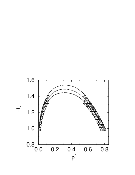
FIG. 4.: Coexistence densities for the polarizable Stockmayer fluids with $|\mathchoice{{\hbox{\boldmath$\displaystyle m_{0}$}}}{{\hbox{\boldmath$\textstyle m_{0}$}}}{{\hbox{\boldmath$\scriptstyle m_{0}$}}}{{\hbox{\boldmath$\scriptscriptstyle m_{0}$}}}^{*}|=1.0$. Circles, squares, triangles are for $\alpha^{*}=$ 0.00, 0.03, and 0.06, respectively. The error bars are about the same or smaller than the size of the symbols. Solid line, dashed line, and dot-dashed line are the results of the Wertheim’s perturbation theory for $\alpha^{*}=$ 0.00, 0.03, and 0.06 respectively.

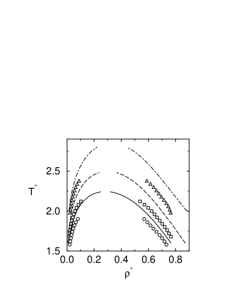
FIG. 5.: Coexistence densities for the polarizable Stockmayer fluids with $|\mathchoice{{\hbox{\boldmath$\displaystyle m_{0}$}}}{{\hbox{\boldmath$\textstyle m_{0}$}}}{{\hbox{\boldmath$\scriptstyle m_{0}$}}}{{\hbox{\boldmath$\scriptscriptstyle m_{0}$}}}^{*}|=2.0$. The notation is the same as in figure 4.

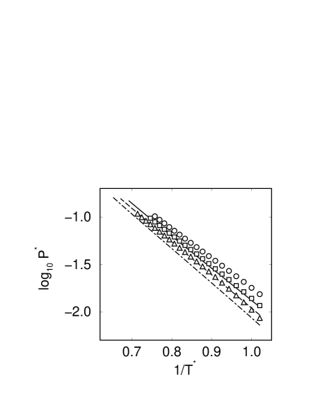
FIG. 6.: Coexistence pressure for the polarizable Stockmayer fluids with $|\mathchoice{{\hbox{\boldmath$\displaystyle m_{0}$}}}{{\hbox{\boldmath$\textstyle m_{0}$}}}{{\hbox{\boldmath$\scriptstyle m_{0}$}}}{{\hbox{\boldmath$\scriptscriptstyle m_{0}$}}}^{*}|=1.0$. The notation is the same as in figure 4.

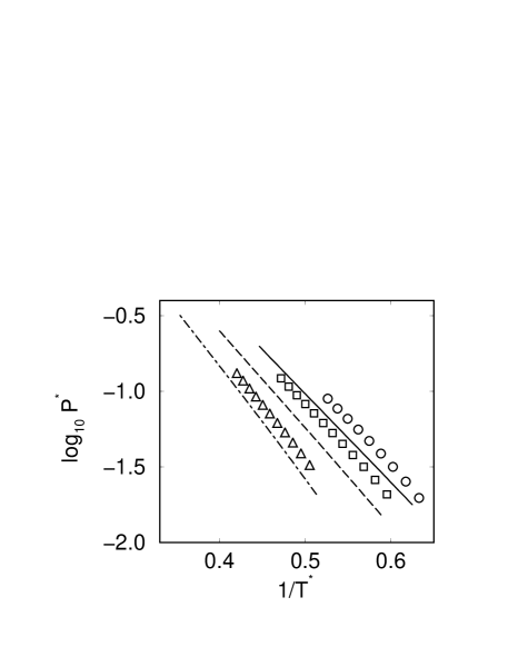
FIG. 7.: Coexistence pressure for the polarizable Stockmayer fluids with $|\mathchoice{{\hbox{\boldmath$\displaystyle m_{0}$}}}{{\hbox{\boldmath$\textstyle m_{0}$}}}{{\hbox{\boldmath$\scriptstyle m_{0}$}}}{{\hbox{\boldmath$\scriptscriptstyle m_{0}$}}}^{*}|=2.0$. The notation is the same as in figure 4.

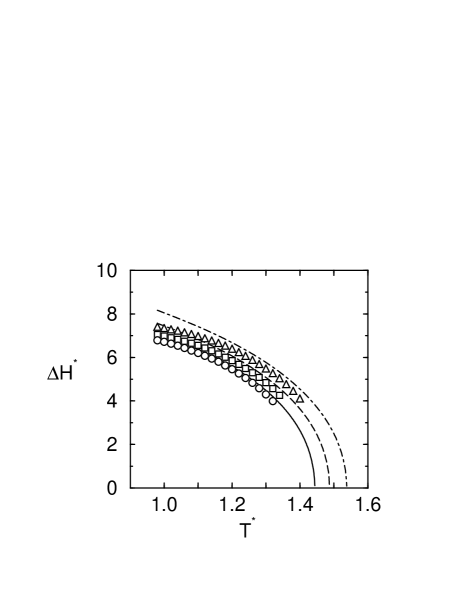
FIG. 8.: Heat of vaporization for the polarizable Stockmayer fluids with $|\mathchoice{{\hbox{\boldmath$\displaystyle m_{0}$}}}{{\hbox{\boldmath$\textstyle m_{0}$}}}{{\hbox{\boldmath$\scriptstyle m_{0}$}}}{{\hbox{\boldmath$\scriptscriptstyle m_{0}$}}}^{*}|=1.0$. The notation is the same as in figure 4.

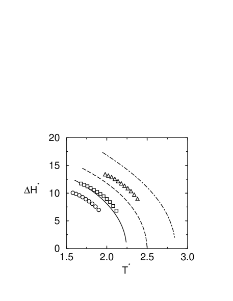
FIG. 9.: Heat of vaporization for the polarizable Stockmayer fluids with $|\mathchoice{{\hbox{\boldmath$\displaystyle m_{0}$}}}{{\hbox{\boldmath$\textstyle m_{0}$}}}{{\hbox{\boldmath$\scriptstyle m_{0}$}}}{{\hbox{\boldmath$\scriptscriptstyle m_{0}$}}}^{*}|=2.0$. The notation is the same as in figure 4.

REFERENCES

- [1] Author for correspondence. E-mail:azp2@cornell.edu
- [2] Stockmayer, W.H. 1941, J. Chem. Phys., 9, 398.
- [3] Rowlinson, J.S., 1949, Trans. Faraday Soc., 45, 974.
- [4] Van Leeuwen, M.E., Ph D thesis, Universiteit Utrecht, The Netherlands, 1995
- [5] Wertheim, M.S., 1973, Molec. Phys., 25, 211 ; Wertheim, M.S., 1977, ibid. 26, 1425 ; Wertheim, M.S., 1977, ibid. 33, 95 ; Wertheim, M.S., 1977, ibid. 34, 1109 ; Wertheim, M.S., 1978, ibid. 36, 1217.
- [6] Wertheim, M.S., 1979, Molec. Phys., 37, 83.
- [7] Venkatasubramanian, V., Gubbins, K.E., Gray, C.G. and Joslin, C.G., 1984, Molec. Phys., 52, 1411.
- [8] Patey, G.N., Torrie, G.M., and Valleau, J.P., 1979, J. Chem. Phys., 71, 96
- [9] Vesely, F.J., 1978, Chem. Phys. Lett., 56, 390.
- [10] Smit, B., Williams, C.P., Hendriks, E.M., and De Leeuw, S.W., 1989 Molec. Phys., 68, 765.
- [11] Van Leeuwen, M.E., Smit, B., and Hendriks, E.M., 1993, Molec. Phys., 78, 271
- [12] Panagiotopoulos, A.Z., 1987, Molec. Phys., 61, 813.
- [13] Torrie, G.M. and Valleau, J.P., 1974, Chem. Phys. Lett., 28, 578; Torrie, G.M. and Valleau, J.P., 1977, J. Comput. Phys., 23, 187:
- [14] Valleau, J.P., 1993, J. Chem. Phys., 99, 4718.
- [15] Widom, B., 1963, J. Chem.Phys., 39, 2808.
- [16] Ferrenberg, A.M. and Swendsen. R.H., 1988, Phys. Rev. Lett., 61, 2635.
- [17] Wilding, N.B., 1995, Phys. Rev. E, 52, 602.
- [18] Norman, G.E. and Filinov, V.S., 1969, High. Temp. 7, 216.
- [19] Metropolis, N., Rosenbluth, A.W., Rosenbluth, M.N., Teller, A.H., and Teller, E., 1953, J.Chem.Phys., 21, 1087.
- [20] Ferrenberg, A.M. and Swendsen. R.H., 1989, Phys. Rev. Lett., 63, 1195.
- [21] Gray, C.G. and Gubbins, K.E., Theory of Molecular Fluids, Vol 1, Clarendon Press, Oxford (1984)
- [22] Bernardo, D.N., Ding, Y., Krogh-Jespersen, K., and Levy, R.M., 1994, J. Phys. Chem., 98, 4180.
- [23] De Leeuw, S.W., Perram, J.W., and Smith, E.R., 1980, Proc. R. Soc. Lond. A 373, 27
- [24] Allen, M.P. and Tiledesley, D.J., 1987, The Computer Simulation of Liquids, (Clarendon, Oxford).
- [25] Johnson, J.K., Zollweg, J.A., and Gubbins, K.E., 1993, Mol. Phys, 78, 591.
- [26] Flytzani-Stephanopoulos, M. and Gubbins, K.E., 1975 Mol. Phys. 30, 1649.
- [27] Gubbins, K.E. and Twu, C.H., 1978, Chem. Eng. Sci. 33, 863.