Optical approximation in the theory of geometric impedance

Abstract

In this paper we introduce an optical approximation into the theory of impedance calculation, one valid in the limit of high frequencies. This approximation neglects diffraction effects in the radiation process, and is conceptually equivalent to the approximation of geometric optics in electromagnetic theory. Using this approximation, we derive equations for the longitudinal impedance for arbitrary offsets, with respect to a reference orbit, of source and test particles. With the help of the Panofsky-Wenzel theorem we also obtain expressions for the transverse impedance (also for arbitrary offsets). We further simplify these expressions for the case of the small offsets that are typical for practical applications. Our final expressions for the impedance, in the general case, involve two dimensional integrals over various cross-sections of the transition. We further demonstrate, for several known axisymmetric examples, how our method is applied to the calculation of impedances. Finally, we discuss the accuracy of the optical approximation and its relation to the diffraction regime in the theory of impedance.

Submitted to Physical Review Special Topics–Accelerators and Beams

I Introduction

The calculation of the impedance for the elements of a vacuum chamber system and the associated calculation of beam dynamics effects, such as beam instabilities or wakefield induced emittance growth, are important elements in the design of a modern accelerator. Sophisticated computer programs are routinely used for such calculations, and in many cases they can successfully treat complicated geometries, like those found in real vacuum systems. There are, however, cases where the simulations are pushed to their limits in resource requirements of both memory and cpu time, and in their ability to yield an accurate result.

One example is the case of very short bunches, like those envisioned in future linear colliders and future light sources. For example, the final bunch length in the current design of the International Linear Collider (ILC) Yokoya (2005) is 300 microns; the final (rms) bunch length in the Linac Coherent Light Source lcl (2002) is 20 microns and in the European XFEL Tes (2002) it is 25 microns. Since numerical calculation of the short-range wake requires a spatial mesh size equal to a fraction of the bunch length, submillimeter bunches represent a challenging computational task. Another example where direct numerical calculation is difficult is related to long, small-angle tapers which are often used to minimize the abruptness of vacuum chamber transitions. For example, collimators with such tapers will be used in the post-linac collimation section of the ILC. In such cases numerical solution of Maxwell’s equations requires a large number of mesh points to fully cover the length of the transition or collimator. The difficulty becomes especially pronounced for short bunches.

The difficulty in both examples mentioned above is associated with a small parameter. For short bunches such a small parameter is the ratio of bunch length $\sigma_{z}$ to typical size $b$ of the structure (in the vacuum chamber) that generates the impedance. If we denote by $\lambdabar$ the inverse wavenumber $c/\omega$ ($c$ is the speed of light and $\omega$ the characteristic frequency of interest) then $\lambdabar\sim\sigma_{z}$, and the small parameter for the problem is $\lambdabar/b$. It has long been known that effective utilization of this small parameter may allow one to simplify the impedance problem, and several analytical results are available in the literature for the impedance at high-frequencies. They include the impedance of a step transition Heifets and Kheifets (1991); Gianfelice and Palumbo (1990) and the diffraction model for the impedance of a cylindrical pillbox cavity Lawson (1990); Palmer (1990); Bane and Sands (1990); Heifets and Kheifets (1990). More recently, a parabolic equation method was developed that provides a simplified treatment of diffraction effects at high-frequencies Stupakov (2006).

In the case of diffraction theory, the calculation takes into account the fact that radiated electromagnetic fields do not propagate along straight lines. A Fresnel type integral from the diffraction theory of light is used to evaluate the electromagnetic energy that enters into the cavity region Lawson (1990); Palmer (1990). This energy is associated with the energy lost by the beam and is thus related to the real part of the impedance. In this paper we will show that in many cases the same kind of argument can be applied to the calculation of impedance in an approximation that we call the optical approximation (or optical regime) in the theory of impedance. In this approximation we assume that the electromagnetic fields carried by a short bunch propagate along straight lines equivalent to rays in the geometric optics. An obstacle inside the beam pipe can intercept the rays and reflect them away from their original direction. The energy in the reflected rays is associated with the energy radiated by the beam, which can then be related to the impedance. Note that this kind of argument has been used in the past in the case of step-in and step-out transitions in a round pipe, where the impedance was related to the energy “clipped away” from the beam by the step Balakin and Novokhatski (1983); Heifets and Kheifets (1990). In a recent paper this approach has been extended and applied to the calculation of impedance for 3D collimators Zagorodnov and Bane (2006).

If $l$ is the length of an obstacle and $b$ is the minimal cross-section size of the beam pipe, the conditions for the optical approximation are

$$\lambdabar\ll b\,,\qquad l\ll\frac{b^{2}}{\lambdabar}\,.$$ (1)

The first of these two conditions requires the size of the obstacle be much larger than the reduced wavelength of the radiation. The right hand side of the second inequality has a meaning of the length over which diffraction effects become significant, and this relation guarantees that such effects give only a small correction to those of geometric optics. Note that even a small-angle taper of angle $\theta\sim b/l$ can be described in the optical approximation for short enough bunches, if $\lambdabar/b\ll\theta$. The quantity ${b^{2}}/{\lambdabar}$ can also be interpreted as a catch-up distance over which radiation, generated by the head of a beam, reflects from a side wall of radius $b$ and reaches the beam tail at length $\sigma_{z}\sim\lambdabar$ behind the head. Thus the second condition of Eq. (1) for the applicability of the optical approximation is that the object is short compared to the catch-up distance.

An analogous problem in geometric optics would be a body with transverse size $b$ and length $l$ illuminated by light, see Fig. 1.

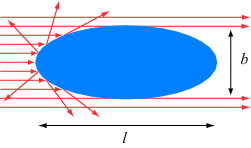
Figure 1: In geometric optics, light incident on a metallic object from the left is reflected by the surface creating a shadow behind the object. The reflected light can be considered as radiation emitted by the object due to currents induced in the metal by the incident electromagnetic field.

The energy reflected by the body can be simply calculated, in the optical approximation, as the energy incident upon the cross-sectional area of the body. Such calculation, however, is only valid if the length of the obstacle $l$ and the transverse size $b$ obey the second condition in Eq. (1). In the opposite limit ($l\gg b^{2}/\lambdabar$), diffraction effects become dominant.

In this paper we assume perfect conductivity in the vacuum chamber wall. Our goal is to justify the optical approximation at high-frequencies and to demonstrate how one can apply it to calculations of both the longitudinal and transverse geometric impedances. We take two approaches to the problem. The first one is based on the general energy balance equation in electromagnetic theory, which relates the longitudinal impedance to the energy radiated from a transition in a beam pipe. In the past, calculations of impedance based on this relation were carried out by one of the authors in axisymmetric Stupakov (1998) as well as rectangular Stupakov (1996) geometries. The derivation is similar to the approach developed in Ref. Huang et al. (2004) for the problem of laser acceleration in vacuum. As it turns out, in the most general case of unequal offsets of the leading and trailing particles, this approach gives the sum of the longitudinal impedances symmetrized over the coordinates of the particles, which does not provide enough information to obtain the transverse impedance for the transition. Our second approach uses a so-called indirect integration method developed in Refs. Zagorodnov (2006); Henke and Bruns (2006). Although not as physically transparent as the energy balance method, this method—with some reasonable assumptions regarding the formation length of the wake field—gives a simple expression for the longitudinal impedance in the most general case.

We want to emphasize here that although our result is not derived formally from first principles, it is based on a combination of exact consequences of Maxwell’s equations and simple physical arguments that follow from the geometric optics. Our result is applicable to an arbitrary three dimensional transition and allows the incoming and outgoing beam pipes to have different cross-sections. Practically important examples of impedance in the optical regime are considered in a companion paper Bane et al. (2007) where we also make a detailed comparison with computer simulations and find excellent agreement between the theory and simulations.

This report is organized as follows. In Section II we derive equations that relate the longitudinal impedance to the integrals of the Fourier transformed Poynting vector over surfaces located far from the transition. In Section III we calculate the contribution to the impedance of the static fields carried by the charges while they are in the incoming and outgoing pipes and far from the transition. The derivation in these two sections is general and does not make any high-frequency assumptions. In Section IV the contribution to the impedance of the radiation field is computed in the optical approximation. In Section V we invoke the indirect integration method to find the wake field for unequal offsets of the particles. In Section VI, using the Panofsky-Wenzel theorem, we derive expressions for the transverse impedance in the optical approximation. Although our results for the transverse impedance are applicable for arbitrarily large transverse offsets, we further specialize them for the case of the small offsets usually assumed in practical applications. Example impedance calculations are given in Section VII where we compute both the longitudinal and transverse impedances of a short, round collimator, and round step-in and step-out transitions. We show that our results for these cases agree with known expressions found in the literature. In Section VIII we discuss the relation between the optical regime and diffraction theory, and establish the accuracy of the optical approximation. Finally, in Section IX we summarize the main results of the paper.

We use Gaussian system of units throughout this paper; to convert impedances to MKS units, one multiplies them by the factor $Z_{0}c/4\pi$, with $Z_{0}=377$ $\Omega$.

II Longitudinal impedance and the energy radiated by charged particles

It is well known that the real part of the longitudinal impedance is related to the energy loss of the beam Chao (1993). Since we assume perfect conductivity in the metallic walls, the losses are due to the beam-induced radiation that propagates away from the transition. In this section we derive a formula that relates the impedance to integrals of the field over remote surfaces far from the transition, and which is valid for a transition of general shape and incoming and outgoing beam pipes of arbitrary cross-section.

We consider transitions between two beam pipes of cross-sections $S_{A}$ and $S_{B}$, respectively, as shown in Fig. 2. $S_{A}$ and $S_{B}$ are arbitrary, other than their axes are parallel to each other and also parallel to the so-called design orbit of the beam. We let the design orbit, in turn, define the $z$-axis.

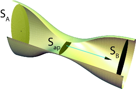
Figure 2: Geometry of a transition from pipe $A$ to pipe $B$. The source and test particles move from left to right along the $z$-axis. The aperture area $S_{\mathrm{ap}}$ is the minimal cross-section that connects the two pipes.

We assume that a charge $q_{1}$ moves at offset $\textnormal{\boldmath$r$}_{1}=(x_{1},y_{1})$ with respect to the design orbit, and a charge $q_{2}$ moves at offset $\textnormal{\boldmath$r$}_{2}=(x_{2},y_{2})$ and at distance $s$ behind (for $s>0$) the leading charge; both charges are assumed to move at the speed of light $c$. We want to calculate the longitudinal wake $w_{\parallel}(\textnormal{\boldmath$r$}_{1},\textnormal{\boldmath$r$}_{2},s)$ given by

$$w_{\parallel}(\textnormal{\boldmath$r$}_{1},\textnormal{\boldmath$r$}_{2},s)=-\frac{c}{q_{1}}\int_{-\infty}^{\infty}E_{1,z}(\textnormal{\boldmath$r$}_{2},z=ct-s,t)dt\,,$$ (2)

where $E_{1,z}(\textnormal{\boldmath$r$},z,t)$ is the $z$-component of the electric field generated by the leading particle at the position of the trailing one. The longitudinal impedance is related to the wake by the Fourier transform

$$Z_{\parallel}(\textnormal{\boldmath$r$}_{1},\textnormal{\boldmath$r$}_{2},\omega)=\frac{1}{c}\int_{0}^{\infty}ds\,w_{\parallel}(\textnormal{\boldmath$r$}_{1},\textnormal{\boldmath$r$}_{2},s)e^{i\omega s/c}\,.$$ (3)

Let us denote the electric and magnetic fields of the leading charge by ${\textnormal{\boldmath$E$}}_{1}(\textnormal{\boldmath$r$},z,t)$ and ${\textnormal{\boldmath$H$}}_{1}(\textnormal{\boldmath$r$},z,t)$, and the electric and magnetic fields of the trailing charge by ${\textnormal{\boldmath$E$}}_{2}(\textnormal{\boldmath$r$},z,t)$ and ${\textnormal{\boldmath$H$}}_{2}(\textnormal{\boldmath$r$},z,t)$. The field $({\textnormal{\boldmath$E$}}_{1},{\textnormal{\boldmath$H$}}_{1})$ is due to the charge density of the first particle, $\rho_{1}=q_{1}\delta(z-ct)\delta(\textnormal{\boldmath$r$}-\textnormal{\boldmath$r$}_{1})$, and the field $({\textnormal{\boldmath$E$}}_{2},{\textnormal{\boldmath$H$}}_{2})$ is generated by the charge density of the second particle, $\rho_{2}=q_{2}\delta(z-s-ct)\delta(\textnormal{\boldmath$r$}-\textnormal{\boldmath$r$}_{2})$. The total field is the sum $\textnormal{\boldmath$E$}={\textnormal{\boldmath$E$}}_{1}+{\textnormal{\boldmath$E$}}_{2}$, $\textnormal{\boldmath$H$}={\textnormal{\boldmath$H$}}_{1}+{\textnormal{\boldmath$H$}}_{2}$.

Using the energy balance equation in electrodynamics Jackson (1999) we can calculate the energy lost by both charges by integrating the Poynting vector over remote boundaries $S_{A}$ and $S_{B}$ located, respectively, far to the left of the incoming pipe and far to the right of the outgoing pipe

$$W=\frac{c}{4\pi}\int_{-\infty}^{\infty}dt\int_{S_{A}+S_{B}}\textnormal{\boldmath$n$}\cdot(\textnormal{\boldmath$E$}\times\textnormal{\boldmath$H$})dS\,.$$ (4)

Here $n$ is the unit vector perpendicular to the surface area, and we use the short-hand notation $\int_{S_{A}+S_{B}}$ for the sum of the integrals over $S_{A}$ and $S_{B}$. In this equation the vector $n$ is oriented in the outward direction—it is parallel (antiparallel) to the $z$ axis on $S_{B}$ ($S_{A}$). A positive value of $W$ means that the charges lose energy. The contribution of such integrals over the metallic surface of the pipes and the transition vanishes because we assume that there are no losses in the wall. It follows from the energy balance equation that the radiated energy given by Eq. (4) is equal to minus the energy change of both particles

$$W=-{cq_{1}}\int_{-\infty}^{\infty}E_{z}(\textnormal{\boldmath$r$}_{1},z=ct,t)dt-{cq_{2}}\int_{-\infty}^{\infty}E_{z}(\textnormal{\boldmath$r$}_{2},z=ct-s,t)dt\,.$$ (5)

The first term in this equation is the energy loss of the leading particle, and the second term is the energy loss for the trailing one. Note that strictly speaking the integration in Eq. (5) should only be performed over the region between the surfaces $S_{A}$ and $S_{B}$; however, assuming that the surfaces are located sufficiently far from the transition (to where the interaction of the charges vanishes), we can extend the limits of integration to infinity.

The electric field at the location of the leading particle is equal to $E_{1,z}(\textnormal{\boldmath$r$}_{1},z=ct,t)+E_{2,z}(\textnormal{\boldmath$r$}_{1},z=ct,t)$, and the electric field at the location of the trailing particle is $E_{1,z}(\textnormal{\boldmath$r$}_{2},z=ct-s,t)+E_{2,z}(\textnormal{\boldmath$r$}_{2},z=ct-s,t)$. We can cast the formula for $W$ as follows:

$$W=q_{1}^{2}U_{1}+q_{1}q_{2}U_{2}+q_{2}^{2}U_{3}\,,$$ (6)

where

$$U_{1} =-\frac{c}{q_{1}}\int_{-\infty}^{\infty}E_{1,z}(\textnormal{\boldmath$r$}_{1},z=ct,t)dt$$

$$U_{2} =-\frac{c}{q_{1}}\int_{-\infty}^{\infty}E_{1,z}(\textnormal{\boldmath$r$}_{2},z=ct-s,t)dt-\frac{c}{q_{2}}\int_{-\infty}^{\infty}E_{2,z}(\textnormal{\boldmath$r$}_{2},z=ct,t)dt$$

$$U_{3} =-\frac{c}{q_{2}}\int_{-\infty}^{\infty}E_{2,z}(\textnormal{\boldmath$r$}_{2},z=ct-s,t)dt\,.$$ (7)

Since we assume that the particles move at the speed of light, due to causality the trailing particle does not affect the leading one. This means that $E_{1,z}(\textnormal{\boldmath$r$}_{2},z=ct-s,t)$ is not equal to zero only if $s>0$, and, similarly, $E_{2,z}(\textnormal{\boldmath$r$}_{2},z=ct,t)$ does not vanish only for $s<0$. This observation allows us to rewrite $U_{2}$ as

$$U_{2}=h(s)w_{\parallel}(\textnormal{\boldmath$r$}_{1},\textnormal{\boldmath$r$}_{2},s)+h(-s)w_{\parallel}(\textnormal{\boldmath$r$}_{2},\textnormal{\boldmath$r$}_{1},-s)\,,$$ (8)

where $h(s)$ is the unit step function.

The next step is to take the Fourier transform in time, introducing the fields $\mathcal{E}$ and $\mathcal{H}$,

$$\left\{\begin{array}[]{r}\textnormal{\boldmath$\mathcal{E}$}(\textnormal{\boldmath$r$},z,\omega)\\ \textnormal{\boldmath$\mathcal{H}$}(\textnormal{\boldmath$r$},z,\omega)\end{array}\right\}=\frac{1}{2\pi}\int_{-\infty}^{\infty}dt\,e^{i\omega t}\left\{\begin{array}[]{r}\textnormal{\boldmath$E$}(\textnormal{\boldmath$r$},z,t)\\ \textnormal{\boldmath$H$}(\textnormal{\boldmath$r$},z,t)\end{array}\right\}\,.$$ (13)

Similarly, we also define the Fourier components $\textnormal{\boldmath$\mathcal{E}$}_{1}(\textnormal{\boldmath$r$},z,\omega)$ and $\textnormal{\boldmath$\mathcal{H}$}_{1}(\textnormal{\boldmath$r$},z,\omega)$ for the electromagnetic field of the first charge. Because the fields $E$ and $H$ are real, we have the relations

$$\textnormal{\boldmath$\mathcal{E}$}(\textnormal{\boldmath$r$},z,-\omega)=\textnormal{\boldmath$\mathcal{E}$}^{*}(\textnormal{\boldmath$r$},z,\omega)\,,\qquad\textnormal{\boldmath$\mathcal{H}$}(\textnormal{\boldmath$r$},z,-\omega)=\textnormal{\boldmath$\mathcal{H}$}^{*}(\textnormal{\boldmath$r$},z,\omega)\,,$$ (14)

with equivalent relations for $\textnormal{\boldmath$\mathcal{E}$}_{1}$ and $\textnormal{\boldmath$\mathcal{H}$}_{1}$. The asterisk in these equations denote complex conjugation. As for the Fourier components of the second charge, we define them in a way that explicitly separates the phase factor introduced by the distance $s$ between the particles:

$$\left\{\begin{array}[]{r}\textnormal{\boldmath$\mathcal{E}$}_{2}(\textnormal{\boldmath$r$},z,\omega)\\ \textnormal{\boldmath$\mathcal{H}$}_{2}(\textnormal{\boldmath$r$},z,\omega)\end{array}\right\}=\frac{1}{2\pi}e^{-i\omega s/c}\int_{-\infty}^{\infty}dte^{i\omega t}\left\{\begin{array}[]{r}\textnormal{\boldmath$E$}_{2}(\textnormal{\boldmath$r$},z,t)\\ \textnormal{\boldmath$H$}_{2}(\textnormal{\boldmath$r$},z,t)\end{array}\right\}\,.$$ (19)

We then have $\textnormal{\boldmath$\mathcal{E}$}=\textnormal{\boldmath$\mathcal{E}$}_{1}+e^{i\omega s/c}\textnormal{\boldmath$\mathcal{E}$}_{2}$ and $\textnormal{\boldmath$\mathcal{H}$}=\textnormal{\boldmath$\mathcal{H}$}_{1}+e^{i\omega s/c}\textnormal{\boldmath$\mathcal{H}$}_{2}$.

From the linearity of Maxwell’s equations it follows that the electromagnetic field $(\textnormal{\boldmath$\mathcal{E}$}_{1},\textnormal{\boldmath$\mathcal{H}$}_{1})$ is generated by the charge density $\hat{\rho}_{1}$ equal to the Fourier image of $\rho_{1}$

$$\hat{\rho}_{1}=\frac{1}{2\pi}\int_{-\infty}^{\infty}dt\,\rho_{1}e^{i\omega t}=\frac{q_{1}}{2\pi c}e^{i\omega z/c}\delta(\textnormal{\boldmath$r$}-\textnormal{\boldmath$r$}_{1})\,,$$ (20)

and the field $(\textnormal{\boldmath$\mathcal{E}$}_{2},\textnormal{\boldmath$\mathcal{H}$}_{2})$ is generated by the charge density

$$\hat{\rho}_{2}=\frac{1}{2\pi}e^{-i\omega s/c}\int_{-\infty}^{\infty}dt\,\rho_{2}e^{i\omega t}=\frac{q_{2}}{2\pi c}e^{i\omega z/c}\delta(\textnormal{\boldmath$r$}-\textnormal{\boldmath$r$}_{2})\,.$$ (21)

Note that because of the extra phase factor $e^{-i\omega s/c}$ in the definition (19) the Fourier components $\hat{\rho}_{1}$ and $\hat{\rho}_{2}$ are now “in phase”. Since $\hat{\rho}_{2}$ has the property $\hat{\rho}_{2}(\omega)=\hat{\rho}_{2}^{*}(-\omega)$, the fields $(\textnormal{\boldmath$\mathcal{E}$}_{2},\textnormal{\boldmath$\mathcal{H}$}_{2})$ satisfy the same relations as Eqs. (14).

Using Parseval’s theorem for Fourier transforms we can express $W$ in Eq. (4) in terms of $\textnormal{\boldmath$\mathcal{E}$}(\omega)$ and $\textnormal{\boldmath$\mathcal{H}$}(\omega)$:

$$W =\frac{c}{2}\int_{-\infty}^{\infty}d\omega\int_{S_{A}+S_{B}}[\textnormal{\boldmath$\mathcal{E}$}(\omega)\times\textnormal{\boldmath$\mathcal{H}$}^{*}(\omega)]\cdot\,\textnormal{\boldmath$n$}\,dS\,,$$ (22)

or, equivalently, in terms of the fields of the first and second particles

$$W =\frac{c}{2}\int_{-\infty}^{\infty}d\omega\int_{S_{A}+S_{B}}[\textnormal{\boldmath$\mathcal{E}$}_{1}(\omega)\times\textnormal{\boldmath$\mathcal{H}$}_{1}^{*}(\omega)]\cdot\,\textnormal{\boldmath$n$}\,dS$$

$$+\frac{c}{2}\int_{-\infty}^{\infty}d\omega\int_{S_{A}+S_{B}}\left[e^{-i\omega s/c}\textnormal{\boldmath$\mathcal{E}$}_{1}(\omega)\times\textnormal{\boldmath$\mathcal{H}$}_{2}^{*}(\omega)+e^{i\omega s/c}\textnormal{\boldmath$\mathcal{E}$}_{2}(\omega)\times\textnormal{\boldmath$\mathcal{H}$}_{1}^{*}(\omega)\right]\cdot\,\textnormal{\boldmath$n$}\,dS$$

$$+\frac{c}{2}\int_{-\infty}^{\infty}d\omega\int_{S_{A}+S_{B}}[\textnormal{\boldmath$\mathcal{E}$}_{2}(\omega)\times\textnormal{\boldmath$\mathcal{H}$}_{2}^{*}(\omega)]\cdot\,\textnormal{\boldmath$n$}\,dS\,.$$ (23)

We will now prove that each of the three terms on the right hand side of Eq. (6) is equal to the corresponding term in Eq. (II). The proof is based on the linearity of Maxwell’s equations and the fact that expressions (6) and (II) are equal for arbitrary values of $q_{1}$ and $q_{2}$. If $q_{2}=0$, then there are only the first terms in these two equations, hence they are equal. If $q_{1}=0$, then there are only the third terms, and they are also equal. Hence the second terms must be equal, too. Using Eq. (8) we obtain

$$h(s)w_{\parallel}(\textnormal{\boldmath$r$}_{1},\textnormal{\boldmath$r$}_{2},s)+h(-s)w_{\parallel}(\textnormal{\boldmath$r$}_{2},\textnormal{\boldmath$r$}_{1},-s)=$$

$$=\frac{c}{2q_{1}q_{2}}\int_{-\infty}^{\infty}d\omega\int_{S_{A}+S_{B}}\left[e^{-i\omega s/c}\textnormal{\boldmath$\mathcal{E}$}_{1}(\omega)\times\textnormal{\boldmath$\mathcal{H}$}_{2}^{*}(\omega)+e^{i\omega s/c}\textnormal{\boldmath$\mathcal{E}$}_{2}(\omega)\times\textnormal{\boldmath$\mathcal{H}$}_{1}^{*}(\omega)\right]\cdot\,\textnormal{\boldmath$n$}\,dS$$

$$=\frac{c}{2q_{1}q_{2}}\int_{-\infty}^{\infty}d\omega\,e^{-i\omega s/c}\int_{S_{A}+S_{B}}\left[\textnormal{\boldmath$\mathcal{E}$}_{1}(\omega)\times\textnormal{\boldmath$\mathcal{H}$}_{2}^{*}(\omega)+\textnormal{\boldmath$\mathcal{E}$}_{2}^{*}(\omega)\times\textnormal{\boldmath$\mathcal{H}$}_{1}(\omega)\right]\cdot\,\textnormal{\boldmath$n$}\,dS\,.$$ (24)

In the last integral we changed the integration variable $\omega\rightarrow-\omega$ in the second term of the integrand and used the relations $\textnormal{\boldmath$\mathcal{E}$}_{2}(-\omega)=\textnormal{\boldmath$\mathcal{E}$}_{2}^{*}(\omega)$ and $\textnormal{\boldmath$\mathcal{H}$}_{1}^{*}(-\omega)=\textnormal{\boldmath$\mathcal{H}$}_{1}(\omega)$. Taking the Fourier transform of this equation and using Eq. (3) gives

$${\cal Z}(\textnormal{\boldmath$r$}_{1},\textnormal{\boldmath$r$}_{2},\omega) \equiv Z_{\parallel}(\textnormal{\boldmath$r$}_{1},\textnormal{\boldmath$r$}_{2},\omega)+Z_{\parallel}(\textnormal{\boldmath$r$}_{2},\textnormal{\boldmath$r$}_{1},\omega)$$

$$=\frac{\pi c}{q_{1}q_{2}}\int_{S_{A}+S_{B}}\left[\textnormal{\boldmath$\mathcal{E}$}_{1}(\omega)\times\textnormal{\boldmath$\mathcal{H}$}_{2}^{*}(\omega)+\textnormal{\boldmath$\mathcal{E}$}_{2}^{*}(\omega)\times\textnormal{\boldmath$\mathcal{H}$}_{1}(\omega)\right]\cdot\,\textnormal{\boldmath$n$}\,dS\,.$$ (25)

The quantity ${\cal Z}$ in this equation is the sum of the impedances symmetrized with respect to the offsets of the leading and trailing particles. If $\textnormal{\boldmath$r$}_{1}=\textnormal{\boldmath$r$}_{2}$, then the left hand side is equal to $2Z_{\parallel}(\textnormal{\boldmath$r$}_{1},\textnormal{\boldmath$r$}_{1},\omega)$ and this equation gives the longitudinal impedance for particles that have the same offset. However, for the general case of unequal offsets, the equation gives only the sum of the impedances ${\cal Z}$.

Note that up to this point we did not use any approximation in our derivation—our result is valid not only in the optical regime, but for arbitrary frequency $\omega$. Eq. (II), relates the sum of two longitudinal impedances to the interference term between the electromagnetic fields of charges 1 and 2 in the energy flow through the remote boundaries $S_{A}$ and $S_{B}$. In the next sections we will split the right hand side of Eq. (II) into several distinct parts and then calculate the parts individually in the optical regime.

III Contribution to impedance of static and radiation fields

There are several contributions to the integral in Eq. (II). The first one comes from the field that is carried by particles when they cross the surface $S_{A}$ on their way to the transition, and the second one arises when they pass through the surface $S_{B}$ after leaving the transition. We call these fields the static fields because they do not vary in time in the beam frame and they can be calculated from a time independent system of equations after a trivial change of variables $z-ct\rightarrow\zeta$ in the laboratory frame. We emphasize here that these are not radiation fields; nevertheless, they need to be included into the original energy balance in Eq. (4).

We begin calculation of the static field contributions from pipe $A$. The electric fields $\textnormal{\boldmath$\mathcal{E}$}_{1,A}$ and $\textnormal{\boldmath$\mathcal{E}$}_{2,A}$ in the straight pipe can be represented in terms of the potential function $\phi$,

$$\textnormal{\boldmath$\mathcal{E}$}_{1,A}=-\frac{q_{1}}{2\pi c}e^{i\omega z/c}\nabla\phi_{1,A}(\textnormal{\boldmath$r$})\,,\qquad\textnormal{\boldmath$\mathcal{E}$}_{2,A}=-\frac{q_{2}}{2\pi c}e^{i\omega z/c}\nabla\phi_{2,A}(\textnormal{\boldmath$r$})\,,$$ (26)

where $\nabla=\textnormal{\boldmath$\hat{x}$}\,\partial/\partial x+\textnormal{\boldmath$\hat{y}$}\,\partial/\partial y$. The potential $\phi$ satisfies Poisson’s equation with source terms given by the charge densities of Eqs. (20) and (21):

$$\nabla^{2}\phi_{1,A}(\textnormal{\boldmath$r$})=-4\pi\delta(\textnormal{\boldmath$r$}-\textnormal{\boldmath$r$}_{1})\,,\qquad\nabla^{2}\phi_{2,A}(\textnormal{\boldmath$r$})=-4\pi\delta(\textnormal{\boldmath$r$}-\textnormal{\boldmath$r$}_{2})\,,$$ (27)

with boundary conditions $\phi_{1,A}=\phi_{2,A}=0$ on the wall of pipe $A$. The magnetic field in pipe $A$ is: $\textnormal{\boldmath$\mathcal{H}$}_{1,A}=\textnormal{\boldmath$\hat{z}$}\times\textnormal{\boldmath$\mathcal{E}$}_{1,A}$ and $\textnormal{\boldmath$\mathcal{H}$}_{2,A}=\textnormal{\boldmath$\hat{z}$}\times\textnormal{\boldmath$\mathcal{E}$}_{2,A}$. We denote by $Z_{A}$ the contribution of these fields, when integrated over the surface $S_{A}$, to the integral Eq. (II)

$$Z_{A} =-\frac{2\pi c}{q_{1}q_{2}}\int_{S_{A}}\textnormal{\boldmath$\mathcal{E}$}_{1}(\omega)\cdot\textnormal{\boldmath$\mathcal{E}$}_{2}^{*}(\omega)dS=-\frac{1}{2\pi c}\int_{S_{A}}\nabla\phi_{1,A}\cdot\nabla\phi_{2,A}\,dS\,.$$ (28)

The minus sign in this equation is due to the fact that the normal vector to $S_{A}$ is oriented in the direction opposite to the $z$ axis.

In the same way we calculate the contribution $Z_{B}$ to Eq. (II) from the remote boundary $S_{B}$. The electric field on this surface $\textnormal{\boldmath$\mathcal{E}$}_{1,B}$ and $\textnormal{\boldmath$\mathcal{E}$}_{2,B}$ is given by the same equations (26) and (27) with the index $A$ replaced by $B$, and the boundary conditions for $\phi_{1,B}$ and $\phi_{2,B}$ being zero on the metallic surface of beam pipe $B$. However, because the direction of the normal vector to $S_{B}$ is along the $z$ axis, $Z_{B}$ has a positive sign

$$Z_{B}=\frac{1}{2\pi c}\int_{S_{B}}\nabla\phi_{1,B}\cdot\nabla\phi_{2,B}\,dS\,.$$ (29)

Note that, strictly speaking, the integrals in Eqs. (28) and (29) diverge because the field has a singularity at the location of charges $q_{1}$ and $q_{2}$. However in the sum $Z_{A}+Z_{B}$ the singular contributions cancel, and the result is finite.

In addition to the terms $Z_{A}$ and $Z_{B}$ there will be a contribution to the impedance due to the radiation field emitted in the transition region. We will denote this contribution $Z_{\mathrm{rad}}$, so that

$${\cal Z}=Z_{A}+Z_{B}+Z_{\mathrm{rad}}\,.$$ (30)

The quantity $Z_{\mathrm{rad}}$ will be evaluated in the next section using the optical approximation.

IV Radiation from the transition in the optical approximation

In the optical regime the radiated energy has several terms. The first term is the energy that is radiated by reflection from the narrowing part of the pipe in the aperture area $S_{\mathrm{ap}}$ (see Fig. 2). We denote the cross-section of the transition that complements $S_{\mathrm{ap}}$ to $S_{A}$ by $S_{A}-S_{\mathrm{ap}}$, and, similarly, the cross-section that complements $S_{\mathrm{ap}}$ to $S_{B}$ by $S_{B}-S_{\mathrm{ap}}$. The incident energy flux within this area will be “clipped away” from the beam and converted into a radiation field. This radiation may go in the backward direction if the narrowing region is steep enough (e.g., a diaphragm, or a 90-degree, abrupt step-in pipe radius), or, for a small-angle taper, it may go in the forward direction. Since the incident energy is the static field in pipe $A$, the contribution $Z_{\mathrm{rad,1}}$ of the clipped energy is given by the same Eq. (28), but with the integration now carried out over the “clipping” area $S_{A}-S_{\mathrm{ap}}$,

$$Z_{\mathrm{rad,1}}=\frac{1}{2\pi c}\int_{S_{A}-S_{\mathrm{ap}}}\nabla\phi_{1,A}\cdot\nabla\phi_{2,A}\,dS\,.$$ (31)

The sign in this equation is positive because the radiation propagates from the transition region to infinity.

Through the aperture $S_{\mathrm{ap}}$ connecting pipes $A$ and $B$, charges carrying the static potential $\phi_{A}$ enter into pipe $B$ (for brevity, we momentarily drop indices 1 and 2). The fields will eventually change in such a way that at a large distance from the transition the particles will carry the potential $\phi_{B}$. In the course of this restructuring, there will be additional radiation emitted in the forward direction. We denote the contribution of this radiation to the impedance by $Z_{\mathrm{rad,2}}$ and calculate it in the following way. We represent the potential of the charges immediately after passing through the aperture as a sum of the potential $\phi_{B}$ occupying area $S_{B}$, the potential $-\phi_{B}$ over the area $S_{B}-S_{\mathrm{ap}}$, and the potential $\phi_{A}-\phi_{B}$ over the area $S_{\mathrm{ap}}$. From the linearity of Maxwell’s equations, the first field proceeds with the charges as a new static field in pipe B, and the last two transform into radiation. The energy integral of the interference fields carrying this radiation is similar to Eqs. (28) and (29) with the difference that over the area $S_{\mathrm{ap}}$ one needs to use $\phi_{A}-\phi_{B}$, and outside of it, the potential $-\phi_{B}$:

$$Z_{\mathrm{rad,2}}=\frac{1}{2\pi c}\int_{S_{\mathrm{ap}}}\nabla(\phi_{1,A}-\phi_{1,B})\cdot\nabla(\phi_{2,A}-\phi_{2,B})\,dS+\frac{1}{2\pi c}\int_{S_{B}-S_{\mathrm{ap}}}\nabla\phi_{1,B}\cdot\nabla\phi_{2,B}\,dS\,.$$ (32)

A slightly different view of the derivation of Eqs. (31) and (32) is illustrated by Fig. 3.

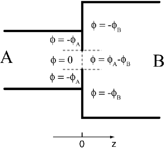
Figure 3: The transition of Fig. 2, represented schematically as an infinitely thin protrusion. Also given are the boundary conditions for the potentials connected to the radiation fields on both the A and B sides of the protrusion.

According to this view, since the length of the transition is short [to satisfy Eqs. (1)], it can be treated as an infinitely short protrusion located at $z=0$. The incident electromagnetic field in pipe A, given by potential $\phi_{A}$, generates a radiation field which will be reflected back into pipe A. The radiation field satisfies the boundary conditions $\phi=-\phi_{A}$ on the left side of the protrusion, at $z=-0$, indicated in Fig. 3. This condition follows from the requirement that the tangential electric field on the surface of the metal is zero. The boundary conditions on the side of pipe B, at $z=+0$, are also indicated in the figure. The radiation field that satisfies these boundary conditions, when summed with the static field corresponding to potential $\phi_{B}$, gives a field equal to zero on the metallic surface of the protrusion, and equal to $\phi_{A}$ over the aperture $S_{ap}$. The interference terms between the radiation fields of the first and the second charges lead to the integrals Eq. (31) and (32) on the left and the right side of the transitions, respectively.

Collecting now all contributions in Eqs. (28), (29), (31) and (32) we arrive at the final result

$${\cal Z}=\frac{1}{\pi c}\int_{S_{B}}\nabla\phi_{1,B}\cdot\nabla\phi_{2,B}\,dS-\frac{1}{2\pi c}\int_{S_{\mathrm{ap}}}\left(\nabla\phi_{1,A}\cdot\nabla\phi_{2,B}+\nabla\phi_{1,B}\cdot\nabla\phi_{2,A}\right)\,dS\,,$$ (33)

where the first integral is carried out over the cross-section of pipe B, and the second integral over aperture $S_{\mathrm{ap}}$. Note that the impedance given by Eq. (33) is real and does not depend on frequency $\omega$.

As was emphasized above, the energy balance equation which was used to derive Eq. (33) gives the summed impedance ${\cal Z}_{\parallel}(\textnormal{\boldmath$r$}_{1},\textnormal{\boldmath$r$}_{2},\omega)=Z_{\parallel}(\textnormal{\boldmath$r$}_{2},\textnormal{\boldmath$r$}_{1},\omega)+Z_{\parallel}(\textnormal{\boldmath$r$}_{1},\textnormal{\boldmath$r$}_{2},\omega)$, which is symmetrized over the offsets of the leading and trailing particles. This suffices to give us the longitudinal impedance for the case when leading and trailing particles follow the same path. However, for the transverse impedance (which we will discuss below) we will need to first find $Z_{\parallel}(\textnormal{\boldmath$r$}_{1},\textnormal{\boldmath$r$}_{2},\omega)$ alone ($\cal Z_{\parallel}$ is not sufficient). To find $Z_{\parallel}(\textnormal{\boldmath$r$}_{1},\textnormal{\boldmath$r$}_{2},\omega)$ in the optical approximation, we will, in the next section, invoke a more formal approach based on a so-called indirect integration method.

V Indirect integration method

The indirect integration method developed in Refs. Zagorodnov (2006); Henke and Bruns (2006) reduces the calculation of the wake field to the integration along a straight path up to some point $z_{0}$ located in the exit pipe B. The contribution from the remaining path $z>z_{0}$ is expressed through the solution of an auxiliary problem at the cross section $z=z_{0}$.

By choosing $z_{0}$ in pipe B immediately after the transition, we note that, in the optical regime, the contribution of path $z<z_{0}$ can be neglected. Indeed, the wake accumulates over the catch up distance $\sim b^{2}/\lambdabar$, which, according to Eqs. (1), is much larger than the transition length $l$. This observation greatly simplifies the problem and allows us to compute the impedance from the part of path with $z>z_{0}$ only. This contribution is Zagorodnov (2006)

$$w(\textnormal{\boldmath$r$}_{1},\textnormal{\boldmath$r$}_{2},s) =-\frac{1}{q_{1}}\Phi(\textnormal{\boldmath$r$}_{2},s)\,,$$ (34)

where $\Phi$ satisfies the equation

$$\nabla^{2}\Phi(\textnormal{\boldmath$r$},s) =\left(\frac{\partial}{\partial z}-c^{-1}\frac{\partial}{\partial t}\right)E_{1,z}^{\mathrm{sc}}(\textnormal{\boldmath$r$},z=0,t=s/c)\ ,$$ (35)

with the boundary condition $\Phi=0$ on the wall of pipe B. The quantity $E_{1}^{\mathrm{sc}}$ is (according to the terminology of Ref. Zagorodnov (2006)) the “scattered” electric field of the leading charge—it is obtained by subtracting from the total field of this charge its static field in pipe B. In Eq. (35) we set $z_{0}=0$ and suppress the argument $\textnormal{\boldmath$r$}_{1}$ in the function $\Phi$—the dependence on this argument is clear from Eq. (35) where the electric field $E_{1,z}$ is generated by the leading particle moving with offset $\textnormal{\boldmath$r$}_{1}$.

We now transform Eq. (35) in a way that eliminates the longitudinal component $E_{z}$. Using $\partial E_{z}^{\mathrm{sc}}/\partial z+\nabla\cdot\textnormal{\boldmath$E$}_{\perp}^{\mathrm{sc}}=0$ and $c^{-1}\partial E_{z}^{\mathrm{sc}}/\partial t=(\nabla\times\textnormal{\boldmath$H$}^{\mathrm{sc}})_{z}$ we obtain

$$\frac{\partial E_{1,z}^{\mathrm{sc}}}{\partial z} =-\nabla\cdot\textnormal{\boldmath$E$}_{1\perp}^{\mathrm{sc}}$$

$$c^{-1}\frac{\partial E_{1,z}^{\mathrm{sc}}}{\partial t} =(\nabla\times\textnormal{\boldmath$H$}_{1\perp}^{\mathrm{sc}})_{z}\,,$$ (36)

where the symbol $\perp$ refers to the components of the field perpendicular to the $z$ axis (we also remind the reader that $\nabla$ is a two-dimensional operator in the $x-y$ plane).

Because we now use the time domain representation for the fields, we need to take the inverse Fourier transform of Eq. (26) (and of a similar equation for pipe B) to find the static fields of the particle. This gives for $\textnormal{\boldmath$E$}_{1}$

$$\textnormal{\boldmath$E$}_{1,A}(\textnormal{\boldmath$r$},z,t)=-\frac{q_{1}}{c}\delta(t-z/c)\nabla\phi_{1,A}(\textnormal{\boldmath$r$})\,,\qquad\textnormal{\boldmath$E$}_{1,B}(\textnormal{\boldmath$r$},z,t)=-\frac{q_{1}}{c}\delta(t-z/c)\nabla\phi_{1,B}(\textnormal{\boldmath$r$})\,,$$ (37)

with the magnetic fields given by $\textnormal{\boldmath$H$}_{1,A}=\textnormal{\boldmath$\hat{z}$}\times\textnormal{\boldmath$E$}_{1,A}$ and $\textnormal{\boldmath$H$}_{1,B}=\textnormal{\boldmath$\hat{z}$}\times\textnormal{\boldmath$E$}_{1,B}$.

The crucial step in the derivation is to notice that, in the optical regime, after passage through the transition region, the static field of particle 1 is “scraped off” outside the aperture $S_{\mathrm{ap}}$. The field left with the charge is equal to $\textnormal{\boldmath$E$}_{1,A}$ but only within the area of $S_{\mathrm{ap}}$ (the field in $S_{B}-S_{\mathrm{ap}}$ is zero). To find the scattered field we need to subtract from the “truncated” field $\textnormal{\boldmath$E$}_{1,A}$ the static field $\textnormal{\boldmath$E$}_{1,B}$ of charge 1 in pipe B, which gives

$$\textnormal{\boldmath$E$}_{1\perp}^{\mathrm{sc}}(\textnormal{\boldmath$r$},z,t)=\begin{cases}-({q_{1}}/{c})\nabla[\phi_{1,A}(\textnormal{\boldmath$r$})-\phi_{1,B}(\textnormal{\boldmath$r$})]\delta(t-z/c)\,\,&\text{in }S_{\mathrm{ap}}\,,\\ -({q_{1}}/{c})\nabla\phi_{1,B}(\textnormal{\boldmath$r$})\delta(t-z/c)&\text{in }S_{B}-S_{\mathrm{ap}}\,,\end{cases}$$ (38)

with the corresponding magnetic field given by

$$\textnormal{\boldmath$H$}_{1\perp}^{\mathrm{sc}}=\textnormal{\boldmath$\hat{z}$}\times\textnormal{\boldmath$E$}_{1\perp}^{\mathrm{sc}}\,.$$ (39)

We substitute Eqs. (38) and (39) into Eq. (V) and use the result as the right hand side in Eq. (35) for $\Phi$. It follows from Eq. (39) that $(\nabla\times\textnormal{\boldmath$H$}_{1\perp}^{\mathrm{sc}})_{z}=\nabla\cdot\textnormal{\boldmath$E$}_{1\perp}^{\mathrm{sc}}$, which gives

$$\nabla^{2}\Phi(\textnormal{\boldmath$r$},s)=-2\nabla\cdot\textnormal{\boldmath$E$}_{1\perp}^{\mathrm{sc}}(\textnormal{\boldmath$r$},z=0,t=s/c)\,.$$ (40)

This equation is solved by first noting that $-(4\pi)^{-1}\phi_{B}(\textnormal{\boldmath$r$})$ is the Green function in $S_{B}$ ($\phi_{B}$ satisfies Eqs. (27) in which A is replaced by B) and then using the symmetry of the Green function with respect to its two arguments Morse and Feshbach (1953). The result is

$$\Phi(\textnormal{\boldmath$r$}_{2},s) =\frac{1}{2\pi}\int_{S_{B}}dS\phi_{2,B}(\textnormal{\boldmath$r$})\nabla\cdot\textnormal{\boldmath$E$}_{1\perp}^{\mathrm{sc}}(\textnormal{\boldmath$r$},z=0,t=s/c)$$

$$=-\frac{1}{2\pi}\int_{S_{B}}dS\nabla\phi_{2,B}(\textnormal{\boldmath$r$})\cdot\textnormal{\boldmath$E$}_{1\perp}^{\mathrm{sc}}(\textnormal{\boldmath$r$},z=0,t=s/c)$$

$$=-\frac{q_{1}}{2\pi}\delta(s)\left[-\int_{S_{ap}}dS\,\nabla\phi_{2,B}\cdot\nabla(\phi_{1,A}-\phi_{1,B})+\int_{S_{B}-S_{ap}}dS\,\nabla\phi_{2,B}\cdot\nabla\phi_{1,B}\right]\,,$$ (41)

where in the second integral we integrated by parts and used the fact that $\phi_{2,B}$ vanishes on the wall of pipe B. Our final result for the wake becomes

$$w=\frac{1}{2\pi}\delta(s)I\,,$$ (42)

where

$$I =\int_{S_{B}}\nabla\phi_{1,B}(\textnormal{\boldmath$r$})\cdot\nabla\phi_{2,B}(\textnormal{\boldmath$r$})\,dS-\int_{S_{ap}}\nabla\phi_{1,A}(\textnormal{\boldmath$r$})\cdot\nabla\phi_{2,B}(\textnormal{\boldmath$r$})\,dS\,.$$ (43)

The impedance corresponding to this wake is

$$Z(\textnormal{\boldmath$r$}_{1},\textnormal{\boldmath$r$}_{2})=\frac{1}{2\pi c}I\,.$$ (44)

It is easy to see that this impedance is consistent with the symmetrized formula Eq. (33).

VI Transverse impedance and small offset of particles

Knowledge of the longitudinal impedance allows one to compute the transverse impedance using the Panofsky-Wenzel theorem Panofsky and Wenzel (1956). In the general case, the transverse impedance is represented by a vector $\textnormal{\boldmath$Z$}_{\perp}$ perpendicular to the particle’s orbit, and is given by

$$\textnormal{\boldmath$Z$}_{\perp}=\frac{c}{\omega}\nabla_{\textnormal{\boldmath$r$}_{2}}Z_{\parallel}\,,$$ (45)

where $\nabla_{\textnormal{\boldmath$r$}_{2}}$ is the operator “nabla” that differentiates with respect to the coordinates $\textnormal{\boldmath$r$}_{2}$ of the trailing particle, $\nabla_{\textnormal{\boldmath$r$}_{2}}=\hat{\textnormal{\boldmath$x$}}\,\partial/\partial x_{2}+\hat{\textnormal{\boldmath$y$}}\,\partial/\partial y_{2}$, with $\hat{\textnormal{\boldmath$x$}}$ and $\hat{\textnormal{\boldmath$y$}}$ being the unit vectors in $x$ and $y$ directions.

In applications, it is typically assumed that there is a symmetry axis in the system and the beam has a small offset relative to this axis compared to the transverse size of the pipe. In this case, one can expand the impedance in Taylor series. The leading terms in the transverse impedance in this case are linear in offsets of the leading and trailing particles. We will now derive expressions for the transverse impedance in this approximation.

For small offsets of the leading and trailing particles we can expand the delta functions in Eqs. (27)

$$\delta(\textnormal{\boldmath$r$}-\textnormal{\boldmath$r$}_{1}) \approx\delta(\textnormal{\boldmath$r$})-\textnormal{\boldmath$r$}_{1}\cdot\nabla\delta(\textnormal{\boldmath$r$})+\frac{1}{2}(\textnormal{\boldmath$r$}_{1}\cdot\nabla)^{2}\delta(\textnormal{\boldmath$r$})\,,$$

$$\delta(\textnormal{\boldmath$r$}-\textnormal{\boldmath$r$}_{2}) \approx\delta(\textnormal{\boldmath$r$})-\textnormal{\boldmath$r$}_{2}\cdot\nabla\delta(\textnormal{\boldmath$r$})+\frac{1}{2}(\textnormal{\boldmath$r$}_{2}\cdot\nabla)^{2}\delta(\textnormal{\boldmath$r$})\,,$$ (46)

and represent each potential as a sum of a monopole part $\phi^{(\mathrm{m})}$, a dipole part $\phi^{(\mathrm{d})}$ and a quadrupole part $\phi^{(\mathrm{q})}$,

$$\phi_{1}=\phi^{(\mathrm{m})}+\phi_{1}^{(\mathrm{d})}+\phi_{1}^{(\mathrm{q})}\,,\qquad\phi_{2}=\phi^{(\mathrm{m})}+\phi_{2}^{(\mathrm{d})}+\phi_{2}^{(\mathrm{q})}\,,$$ (47)

where the parts satisfy the equations:

$$\nabla^{2}\phi^{(\mathrm{m})} =-4\pi\delta(\textnormal{\boldmath$r$})\,,$$

$$\nabla^{2}\phi_{1}^{(\mathrm{d})} =4\pi\textnormal{\boldmath$r$}_{1}\cdot\nabla\delta(\textnormal{\boldmath$r$})\,,\hskip 61.17325pt\nabla^{2}\phi_{2}^{(\mathrm{d})}=4\pi\textnormal{\boldmath$r$}_{2}\cdot\nabla\delta(\textnormal{\boldmath$r$})\,,$$

$$\nabla^{2}\phi_{1}^{(\mathrm{q})} =-2\pi(\textnormal{\boldmath$r$}_{1}\cdot\nabla)^{2}\delta(\textnormal{\boldmath$r$})\,,\hskip 42.67912pt\nabla^{2}\phi_{2}^{(\mathrm{q})}=-2\pi(\textnormal{\boldmath$r$}_{2}\cdot\nabla)^{2}\delta(\textnormal{\boldmath$r$})\,.$$ (48)

Representation (47) generates many terms in Eq. (44). The linear term in $\textnormal{\boldmath$r$}_{2}$ after substitution into the Panofsky-Wenzel Eq. (45) gives rise to a transverse impedance which corresponds to a kick on particle 2 when both particles travel along the reference orbit without offset. We will call this impedance the transverse monopole impedance and denote the corresponding longitudinal impedance by $Z_{\parallel,m}$, where

$$Z_{\parallel,m} =\frac{1}{2\pi c}\int_{S_{B}}\nabla\phi_{1,B}^{(\mathrm{m})}\cdot\nabla\phi_{2,B}^{(\mathrm{d})}\,dS-\frac{1}{2\pi c}\int_{S_{\mathrm{ap}}}\nabla\phi_{1,A}^{(\mathrm{m})}\cdot\nabla\phi_{2,B}^{(\mathrm{d})}\,dS\,.$$ (49)

In many practical cases the structure geometry has both up-down and right-left symmetry and the design orbit is on the symmetry line. In such a case the transverse monopole impedance vanishes. The longitudinal impedance which gives the usual transverse wake then has a term that is proportional to the product of vector components of $\textnormal{\boldmath$r$}_{2}$ and $\textnormal{\boldmath$r$}_{1}$ and one that is quadratic in $\textnormal{\boldmath$r$}_{2}$ (no dependence on $\textnormal{\boldmath$r$}_{1}$). According to accepted terminology, we will call the former (in the case of impedance) the dipole component, $Z_{\parallel,d}$, and the latter the quadrupole component, $Z_{\parallel,q}$. The total impedance, the sum of the two components, is given by

$$Z_{\parallel}=Z_{\parallel,d}+Z_{\parallel,q}\,,$$ (50)

where

$$Z_{\parallel,d} =\frac{1}{2\pi c}\int_{S_{B}}\nabla\phi_{1,B}^{(\mathrm{d})}\cdot\nabla\phi_{2,B}^{(\mathrm{d})}\,dS-\frac{1}{2\pi c}\int_{S_{\mathrm{ap}}}\nabla\phi_{1,A}^{(\mathrm{d})}\cdot\nabla\phi_{2,B}^{(\mathrm{d})}\,dS\,,$$ (51)

and

$$Z_{\parallel,q} =\frac{1}{2\pi c}\int_{S_{B}}\nabla\phi_{1,B}^{(\mathrm{m})}\cdot\nabla\phi_{2,B}^{(\mathrm{q})}\,dS-\frac{1}{2\pi c}\int_{S_{\mathrm{ap}}}\nabla\phi_{1,A}^{(\mathrm{m})}\cdot\nabla\phi_{2,B}^{(\mathrm{q})}\,dS\,.$$ (52)

Note that for the special case of cylindrically symmetric structures the quadrupole component is identically equal to zero.

Equations (45), (49), (51), and (52) allows one to calculate all the component of the transverse impedance for a transition of arbitrary geometry.

VII Example impedance calculations in the optical regime

In this section we will show how to calculate the longitudinal and transverse impedances for several simple cases of axisymmetric systems using results of Section VI.

We first calculate the longitudinal impedance for a short, round collimator shown in Fig. 4a,

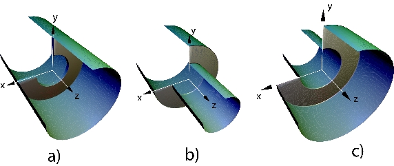
Figure 4: A short collimator (a), a step-in (b), and a step-out (c) transition in axisymmetric geometry. The particles move in the $+z$ direction. For the collimator $a$ denotes the pipe radius and $b$ the collimator radius, with $b<a$. For the step transitions, $a$ denotes the radius of the incoming pipe and $b$ the radius of the outgoing pipe, with $b<a$ for the step-in and $b>a$ for the step-out transition.

with pipe radius $a$ and collimator radius $b$ ($b<a$). In this case both charges are located on the axis of the pipe, and the solution to Eqs. (27), in cylindrical coordinates, is

$$\phi_{1,2}=-2\ln\frac{r}{a}\,.$$ (53)

Substituting this solution into Eq. (44) yields

$$Z_{\parallel} =\frac{1}{2\pi c}\int_{S_{B}}(\nabla\phi_{1})^{2}\,dS-\frac{1}{2\pi c}\int_{S_{\mathrm{ap}}}(\nabla\phi_{1})^{2}\,dS$$

$$=\frac{1}{2\pi c}\int_{S_{B}-S_{\mathrm{ap}}}(\nabla\phi_{1})^{2}\,dS=\frac{4}{c}\ln\frac{a}{b}\,.$$ (54)

This is a well known result for the collimator impedance in the high frequency limit.

The longitudinal impedance for step-in and step-out transitions shown in Fig. 4b and 4c can easily be obtained from the previous equations. In both cases the potential $\phi$ is $-2\ln(r/a)$ and $-2\ln(r/b)$ for pipes of radius $a$ and $b$, respectively. However, for the step-in transition, the cross-section $S_{B}$ coincides with $S_{\mathrm{ap}}$, and the two integrals in Eq. (43) cancel, giving a total impedance of zero. For a step-out transition, the difference of these integrals is the same as given by the first line in Eq. (VII), and the impedance is equal to that of a collimator with the aperture equal to the radius of pipe B. Again, both these results are known in the literature, and we have derived them here to demonstrate that the optical approximation agrees with previously obtained results.

For the transverse impedance of a round collimator and a step-in and a step-out transition we first note that only the dipole term in Eq. (50) contributes to the impedance. The quadrupole term in this equation vanishes because the monopole potential $\phi^{(\mathrm{m})}$ in Eq. (52) has no angular dependence while the quadrupole potential $\phi^{(\mathrm{q})}$ has an angular dependence $\propto\cos 2\theta$ (here $\theta$ is the azimuthal angle in cylindrical coordinates).

For a round collimator, pipe A and pipe B have the same radius $a$, hence, $\phi_{1,A}^{(\mathrm{d})}=\phi_{1,B}^{(\mathrm{d})}$ and $\phi_{2,A}^{(\mathrm{d})}=\phi_{2,B}^{(\mathrm{d})}$. This reduces the integration in Eq. (51) to one over the collimator area

$$Z_{\parallel,d} =\frac{1}{2\pi c}\int_{S_{B}-S_{\mathrm{ap}}}\nabla\phi_{1,A}^{(\mathrm{d})}\cdot\nabla\phi_{2,A}^{(\mathrm{d})}\,dS\,.$$ (55)

We assume now that both leading and trailing particles are offset in the direction of the $x$ axis and define function $\psi$ such that

$$\phi_{1,A}^{(\mathrm{d})}=x_{1}\psi_{A}\,,\qquad\phi_{2,A}^{(\mathrm{d})}=x_{2}\psi_{A}\,.$$ (56)

The function $\psi_{A}$ satisfies the following equation

$$\nabla^{2}\psi_{A}=4\pi\delta^{\prime}(x)\delta(y)\,,$$ (57)

where the prime denotes derivative with respect to the argument, with the boundary condition $\psi_{A}=0$ at $r=a$. The solution is

$$\psi_{A}=-2x\left(\frac{1}{a^{2}}-\frac{1}{x^{2}+y^{2}}\right)=-2r\cos\theta\left(\frac{1}{a^{2}}-\frac{1}{r^{2}}\right)\,.$$ (58)

The expressions (56) are next substituted into Eq. (55) and integrated over the cross-sectional area of the collimator. The calculation can be simplified if one uses the identity

$$\int_{S_{B}-S_{\mathrm{ap}}}\nabla\psi_{A}\cdot\nabla\psi_{A}\,dS=\int_{S_{B}-S_{\mathrm{ap}}}\nabla\cdot(\psi_{A}\nabla\psi_{A})\,dS-\int_{S_{B}-S_{\mathrm{ap}}}\psi_{A}\nabla^{2}\psi_{A}\,dS\,.$$ (59)

The second integral on the right hand side vanishes because $\nabla^{2}\psi_{A}=0$ in any region that does not include the point $x=y=0$, and the first one can be cast into an integral over the edge of the collimator $r=b$

$$\int_{S_{B}-S_{\mathrm{ap}}}\nabla\cdot(\psi_{A}\nabla\psi_{A})\,dS=-b\int_{0}^{2\pi}\psi_{A}\frac{\partial\psi_{A}}{\partial r}\,d\theta=\frac{4\pi}{b^{2}}\left(1-\frac{b^{4}}{a^{4}}\right)\,,$$ (60)

which gives for the longitudinal dipole impedance

$$Z_{\parallel,d} =x_{1}x_{2}\frac{2}{cb^{2}}\left(1-\frac{b^{4}}{a^{4}}\right)\,.$$ (61)

Using now the Panofsky-Wenzel relation Eq. (45) we find the $x$ component of the transverse impedance

$$\frac{Z_{\perp,x}}{x_{1}} =\frac{2}{\omega b^{2}}\left(1-\frac{b^{4}}{a^{4}}\right)\,.$$ (62)

The right hand side of this equations defines the transverse impedance per unit offset $x_{1}$—this quantity is traditionally referred to as the transverse impedance. The result Eq. (62) agrees with Ref. Zagorodnov and Bane (2006).

For the step-in and step-out transitions, Eqs. (56) and (58) define the dipole potentials for pipe A; the potentials for pipe B are obtained from these formulae by exchanging $b$ and $a$,

$$\phi_{1,B}^{(\mathrm{d})} =x_{1}\psi_{B}\,,\qquad\phi_{2,B}^{(\mathrm{d})}=x_{2}\psi_{B}$$

$$\psi_{B} =-2x\left(\frac{1}{b^{2}}-\frac{1}{x^{2}+y^{2}}\right)=-2r\cos\theta\left(\frac{1}{b^{2}}-\frac{1}{r^{2}}\right)\,.$$ (63)

Note that the difference $\Delta\psi=\psi_{A}-\psi_{B}$ corresponds to a uniform electric field in the $x$ direction

$$\Delta\psi=2x\left(\frac{1}{b^{2}}-\frac{1}{a^{2}}\right)\,.$$ (64)

For the step-in transition $S_{\mathrm{ap}}=S_{B}$, and after a simple transformation Eq. (51) can be reduced to

$$Z_{\parallel,d} =-\frac{x_{1}x_{2}}{2\pi c}\int_{S_{B}}\left(\nabla\Delta\psi\cdot\nabla\psi_{B}\right)\,dS\,.$$ (65)

Using the same integration by parts as in Eq. (59) we obtain

$$\int_{S_{B}}\left(\nabla\Delta\psi\cdot\nabla\psi_{B}\right)\,dS =\int_{S_{B}}\nabla\cdot\left(\Delta\psi\nabla\psi_{B}\right)\,dS-\int_{S_{B}}\left(\Delta\psi\nabla^{2}\psi_{B}\right)\,dS$$

$$=b\int_{0}^{2\pi}\Delta\psi{\left.\frac{\partial\psi_{B}}{\partial r}\right|_{r=b}}\,d\theta-4\pi\int_{S_{B}}\Delta\psi\delta^{\prime}(x)\delta(y)\,dS$$

$$=0\,,$$ (66)

which means that the longitudinal dipole impedance, and hence the transverse impedance, is equal to zero for the step-in transition. We remind the reader that the longitudinal impedance for this case also vanishes.

For the step-out transition $S_{\mathrm{ap}}=S_{A}$. We represent the integral over $S_{\mathrm{ap}}$ in Eq. (51) as the difference of the integrals over $S_{B}$ and the integral over $S_{B}-S_{\mathrm{ap}}$. Then the first term in this equation combined with the integrals over $S_{B}$ gives zero, as follows from the calculations for the step-in transition. Hence

$$Z_{\parallel,d} =\frac{x_{1}x_{2}}{2\pi c}\int_{S_{B}-S_{\mathrm{ap}}}\left(\nabla\psi_{A}\cdot\nabla\psi_{B}\right)\,dS$$

$$=\frac{x_{1}x_{2}}{2\pi c}\int_{S_{B}-S_{\mathrm{ap}}}\nabla\cdot\left(\psi_{A}\nabla\psi_{B}\right)\,dS$$

$$=\frac{x_{1}x_{2}}{2\pi c}b\int_{0}^{2\pi}\left.\psi_{A}\frac{\partial\psi_{B}}{\partial r}\right|_{r=b}\,d\theta$$

$$=\frac{4x_{1}x_{2}}{c}\left(\frac{1}{a^{2}}-\frac{1}{b^{2}}\right)\,.$$ (67)

For the transverse impedance in this case we find

$$\frac{Z_{\perp,x}}{x_{1}} =\frac{4}{\omega a^{2}}\left(1-\frac{a^{2}}{b^{2}}\right)\,,$$ (68)

which agrees with the result of Ref. Gianfelice and Palumbo (1990).

VIII Pillbox cavity and relation between optical and diffraction regimes

Let us consider now the pillbox cavity shown in Fig. 5.

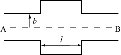
Figure 5: An axisymmetric pillbox cavity.

Diffraction theory gives the longitudinal impedance for a cavity as (see, e.g. Chao (1993))

$$Z_{\parallel,\mathrm{diffraction}}=\frac{2(1+i)}{\pi^{1/2}}\sqrt{\frac{l}{cb^{2}\omega}}\,,$$ (69)

where $b$ is the pipe radius and $l$ is the length of the cavity.

The optical theory predicts zero impedance for the pillbox cavity. Indeed, in this case, all the three cross-sections $S_{A}$, $S_{\mathrm{ap}}$ and $S_{B}$ are equal (regarding the determination of $S_{\mathrm{ap}}$ in this case see the footnote on page 2), and Eq. (43) immediately gives a zero result. The reason for the optical approximation not reproducing the result of the diffraction theory is that Eq. (69) corresponds to the next order approximation in the small parameter $\lambdabar l/b^{2}$, which is beyond the applicability limit of the optical regime. Indeed, if we take the ratio of the impedance Eq. (69) to a typical optical impedance $Z_{\parallel,\mathrm{optical}}\sim 1/c$ [see, e.g. Eq. (VII)], we obtain

$$\frac{Z_{\parallel,\mathrm{diffraction}}}{Z_{\parallel,\mathrm{optical}}}\sim\sqrt{\frac{lc}{b^{2}\omega}}\sim\sqrt{\frac{l\lambdabar}{b^{2}}}\,.$$ (70)

Hence the parameter $\sqrt{{l\lambdabar}/{b^{2}}}$ indicates the accuracy of the optical approximation: one can expect that corrections to the optical regime due to diffraction effects will be on the order of this parameter.

Note that one can find in the literature references to the impedance of the collimator given by Eq. (VII) as a diffraction impedance (the authors of this paper have also used this terminology in the past). The terminology introduced in this paper distinguishes the optical regime from the diffraction regime, and we believe that it better describes the physics involved.

IX Conclusion

In this paper we have introduced an optical approximation into the theory of impedance calculation, valid in the limit of high frequencies. This approximation neglects diffraction effects in the radiation process, and is conceptually equivalent to the approximation of geometric optics in electromagnetic theory. Using this approximation, we have derived equations for the longitudinal impedance for arbitrary offsets of the source and test particles with respect to a reference orbit. With the help of the Panofsky-Wenzel theorem we have also obtained expressions for the transverse impedance (also for arbitrary offsets). We further simplified these expressions for the case of the small offsets that are typical for practical applications. Our final expressions for the impedance, in the general case, involve two dimensional integrations over various cross-sections of the transition.

We have, in addition, demonstrated for several simple examples how our method is applied to the calculation of impedances for simple axisymmetric geometries that have been studied in the past. Finally, we discussed the accuracy of the optical approximation and its relation to the diffraction regime in the theory of impedance.

References

• Yokoya (2005) K. Yokoya, in 2005 International Linear Collider Physics and Detector Workshop and Second ILC Accelerator Workshop (Snowmass, CO, 2005).
• lcl (2002) Report SLAC-R-593, SLAC (2002).
• Tes (2002) Report DESY-2002-167, DESY (2002).
• Heifets and Kheifets (1991) S. A. Heifets and S. A. Kheifets, Review of Modern Physics 63, 631 (1991).
• Gianfelice and Palumbo (1990) E. Gianfelice and L. Palumbo, IEEE Trans. Nucl. Sci. 37, 1081 (1990).
• Lawson (1990) J. D. Lawson, Part. Accel. 25, 107 (1990).
• Palmer (1990) R. B. Palmer, Part. Accel. 25, 97 (1990).
• Bane and Sands (1990) K. Bane and M. Sands, Part. Accel. 25, 73 (1990).
• Heifets and Kheifets (1990) S. A. Heifets and S. A. Kheifets, Part. Accel. 25, 61 (1990).
• Stupakov (2006) G. Stupakov, New Journal of Physics 8, 280 (2006).
• Balakin and Novokhatski (1983) V. E. Balakin and A. V. Novokhatski, in Proceedings of the 12th International Conference on High-Energy Accelerators, edited by F. T. Cole and R. Donaldson (Fermilab, Batavia, IL, 1983), p. 117.
• Zagorodnov and Bane (2006) I. Zagorodnov and K. L. F. Bane, in Proc. European Particle Accelerator Conference, Edinburgh, 2006 (2006), pp. 2859–2861.
• Stupakov (1998) G. V. Stupakov, Phys. Rev. ST Accel. Beams 1, 064401 (1998).
• Stupakov (1996) G. Stupakov, Preprint SLAC-PUB-7167, SLAC (1996).
• Huang et al. (2004) Z. Huang, G. Stupakov, and M. Zolotorev, Phys. Rev. ST Accel. Beams 7, 011302 (2004).
• Zagorodnov (2006) I. Zagorodnov, Phys. Rev. ST Accel. Beams 9, 102002 (2006).
• Henke and Bruns (2006) H. Henke and W. Bruns, in Proc. European Particle Accelerator Conference, Edinburgh, 2006 (2006), pp. 2171–2172.
• Bane et al. (2007) K. Bane, G. Stupakov, and I. Zagorodnov, Preprint 12370, SLAC (2007).
• Chao (1993) A. W. Chao, Physics of Collective Beam Instabilities in High Energy Accelerators (Wiley, New York, 1993).
• Jackson (1999) J. D. Jackson, Classical Electrodynamics (Wiley, New York, 1999), 3rd ed., page 259.
• Morse and Feshbach (1953) P. M. Morse and H. Feshbach, Methods of theoretical physics (McGraw-Hill, 1953), 2nd ed., vol. 1, page 873.
• Panofsky and Wenzel (1956) W. K. H. Panofsky and W. Wenzel, Rev. Sci. Instr. 27, 967 (1956).