Implementation of a double-scanning technique
for studies of the Hanle effect in Rubidium vapor

Abstract

We have studied the resonance fluorescence of a room-temperature rubidium vapor exited to the atomic ⁵P_3/2 state (D₂ line) by powerful single-frequency cw laser radiation (1.25 W/cm²) in the presence of a magnetic field. In these studies, the slow, linear scanning of the laser frequency across the hyperfine transitions of the D₂ line is combined with a fast linear scanning of the applied magnetic field, which allows us to record frequency-dependent Hanle resonances from all the groups of hyperfine transitions including V- and $\Lambda$ - type systems. Rate equations were used to simulate fluorescence signals for ⁸⁵Rb due to circularly polarized exciting laser radiation with different mean frequency values and laser intensity values. The simulation show a dependance of the fluorescence on the magnetic field. The Doppler effect was taken into account by averaging the calculated signals over different velocity groups. Theoretical calculations give a width of the signal peak in good agreement with experiment.

I Introduction

Sustained interest in resonant magneto-optical effects in atomic vapors is due to their importance to fundamental physics but also to possibility of using these effects in numerous applications (see  Mor91 ; Ale93 ; Bud02 ; Ale05 and references therein). Besides the obvious dependence on the applied magnetic field, the resonant nature of these effects implies a substantial dependence on the laser frequency. Meanwhile, as a rule, only one or two of these parameters is varied in a given experimental measurement. In the present work, we report the results of an investigation of the nonlinear Hanle effect Pap02 ; Aln03 where both the laser frequency and the magnetic field were scanned continuously and simultaneously at different sequence rates And07 . This technique enables us to acquire additional information in one measurement sequence , and can help to better understand and model the processes under study. This technique can be applied to other magneto-optical effects as well Pap06 .

Usually, models of nonlinear magneto-optical effects are based on the optical Bloch equations Ste05 . At the same time, as was shown in Blu04 , simpler rate equations for Zeeman coherences for stationary or quasi-stationary excitation are equivalent to the optical Bloch equations. The model based on the rate equations was successfully applied to studies of atomic interactions with laser radiation in cells in the presence of an external magnetic field Aln01 ; Pap02 ; Aln03 .

The elaboration of a realistic model of the interaction of alkali atoms with laser radiation is complicated by the fact that the fine structure levels of a typical alkali atom consists of several hyperfine structure (HFS) levels that in experiments in cells can be only partially resolved spectroscopically due to Doppler broadening. If an external magnetic field is applied, the situation becomes even more complicated. The magnetic field mixes together magnetic sublevels with the same magnetic quantum number $M$, but belonging to different hyperfine states. This mixing can be quite strong, as was shown experimentally and confirmed in a model for Rb atoms Sar05 confined in an extremely thin cell Sar01 . In that study the extremely thin cell allowed to resolve spectroscopically transitions between specific magnetic sublevels. When scanning the laser frequency there appeared in a fluorescence excitation spectrum transitions that would not be allowed in the absence of the level mixing due to magnetic field.

In the present study we propose to show that in the model of the nonlinear Hanle effect we have for the first time accounted simultaneously for all these effects, namely, the creation of Zeeman coherences between magnetic sublevels in the ground and excited states, the mixing of the different hyperfine levels in the magnetic field (partial decoupling of the electronic angular momentum of the electrons from the nuclear spin), and the Doppler effect in the manifold of magnetic sublevels of all hyperfine levels of the fine structure states involved.

II Experiment

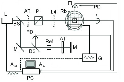
Figure 1: Experimental Setup. Abbreviations: L- laser, BS- beam splitter ,AT- attenuator, P- polarizer, L4- $\lambda$/4 plate, Rb - Rubidium cell in Helmholtz coils,Fl- fluorescence detector, PD- photodiode, M- 100 % mirror, Ref- reference Rb cell, G- generator / booster,A_in - analog in, A_out - analog out.

II.1 Experimental details

A schematic drawing of the experimental setup is shown in Fig. 1. A radiation beam from the solitary laser diode (Sanyo^TM DL-7140-201 W) was directed into the $1$ cm-long glass cell containing natural rubidium. The temperature of the cell was $T_{cell}=24$ C ($N_{Rb}$ = $8.6\times 10^{9}$ cm^-3). The measured output power was $45$ mW at the Rb D₂ line, the spectral linewidth was $\sim 15$ MHz, and the laser beam diameter was $1.5$ mm. The cell was placed in $3$ mutually orthogonal pairs of Helmholtz coils without metal shielding, which reduced the dc magnetic field to $\sim 10$ mG and could apply a magnetic field of up to $80$ G in a chosen direction. The resonant fluorescence emerging from the cell was detected by a photodiode placed at an angle of $90$ degrees to the laser beam, $14$ cm from the cell. The detection solid angle was $0.004$ srad. The total intensity of the laser induced fluorescence was measured without spectral or polarization selection. It was possible to simultaneously record also the transmitted signal and the saturated absorption signal (branched to an auxiliary setup, as shown in Fig. 1). Control of the diode laser injection current and hence, the radiation frequency, as well as data acquisition were done by means of virtual function generator and a multi-channel oscilloscope, with the help of a National Instruments^TM DAQ board installed in the PC. The software was written in LabVIEW^TM . The measurements were performed by linearly scanning the laser frequency over a $6$ GHz range around the Rb D₂ line, covering the ⁸⁷Rb $F_{g}=2\rightarrow F_{e}=1,2,3$, ⁸⁵Rb $F_{g}=3\rightarrow F_{e}=2,3,4,$ and ⁸⁵Rb $F_{g}=2\rightarrow F_{e}=1,2,3$ Doppler-broadened and partially overlapping transitions. The typical duration of a one-way scan was $5$ s. Within this time period, the magnetic field is periodically scanned by 120 triangular bipolar pulses, each with a duration of of $41.5$ ms. The number of measurement points per frequency scan was $50000$ (over $400$ points per magnetic field scan). The fluorescence measurement in one scanning point takes $100$ $\mu$s. This measurement time interval is sufficiently large to allow good signal resolution and the development of a steady state interaction regime. The mutual orientation of the laser radiation, its polarization, and the direction of the magnetic field is shown in Fig.2.

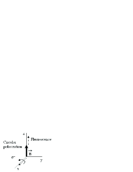
Figure 2: Excitation light propagation, magnetic field and fluorescence detection geometry.

II.2 Experimental Results

Figure 3: Fluorescence signal for circular polarized excitation light when simultaneously scanning the mean frequency $\bar{\omega}$ of the laser light and the magnetic field B.

Figure 3 show the double-scanning fluorescence excitation spectra for the circularly polarized excitation recorded with laser intensity $I_{L}=1.25$ W/cm². We can clearly see fluorescence coming from the excitation of ⁸⁷Rb atoms in the ground state level $F_{g}=2$, as well as fluorescence coming from the excitation of ⁸⁵Rb atoms in the ground state levels $F_{g}=3$ and $F_{g}=2$. Vertical lines in the graph show frequencies of atomic transitions for atoms at rest. For example, line ”$3-4$” shows the position of the transition $F_{g}=3\rightarrow F_{e}=4$ for ⁸⁵Rb atoms. In this figure it can be seen that the structure of the nonlinear Hanle signal depends on ground state HFS level from which it was excited. The Hanle signals for excitation from the ⁸⁷Rb $F_{g}=2$ and from the ⁸⁵Rb $F_{g}=3$ levels exhibit sharp, high-contrast peaks in the vicinity of zero magnetic field. The inset in Fig. 3 shows the dependance of the fluorescence on the magnetic field in the vicinity of these peaks. The width of these high-contrast peaks is about $2$ G. In contrast, the fluorescence excited from the ground state HFS level $F_{g}=2$ of ⁸⁵Rb exhibits dips in the vicinity of zero magnetic field of approximately the same width as the previously discussed peaks. For each of the three Doppler-overlapped groups of the three HFS transitions, sub-Doppler dips appear at high laser intensity, located at the frequency positions of the two crossover resonances linked by the cycling transitions. As was shown (but not comprehensively explained) in Pap99 , these dips arise even if precautions are taken to eliminate the backward-reflected beam from the cell, as was done also in this work.

Similar spectra to the double-scanning fluorescence excitation spectra depicted in Fig. 3 were taken in the laser intensity range from $70$ mW/cm² up to $1.25$ W/cm².

III Theoretical Model

III.1 Outline of the model

In order to build a model of the nonlinear Hanle effect in Rb atoms in a cell, we will explore the concept of the density matrix of an atomic ensemble. The diagonal elements of the density matrix $\rho_{ii}$ of an atomic ensemble describe the population of a certain atomic level $i$, and the non-diagonal elements $\rho_{ij}$ describe coherences created between the levels $i$ and $j$. In our particular case the level in question are magnetic sublevels of a certain HFS level. If atoms are excited from the ground state HFS level $g$ to the excited state HFS level $e$, then the density matrix consists of elements $\rho_{g_{i}g_{j}}$ and $\rho_{e_{i}e_{j}}$, called Zeeman coherences, as well as ”cross-elements” $\rho_{g_{i}e_{j}}$, called optical coherences.

The optical Bloch equations (OBEs) can be written as Ste05 :

$$i\hbar\dfrac{\partial\rho}{\partial t}=\left[\widehat{H},\rho\right]+i\hbar\widehat{R}\rho,$$ (1)

where the operator $\widehat{R}$ represents the relaxation matrix. If an atom interacts with laser light and an external dc magnetic field, we can write the Hamiltonian $\widehat{H}=\widehat{H}_{0}+\widehat{H}_{B}+\widehat{V}$. $\widehat{H}_{0}$ is the unperturbed atomic Hamiltonian, which depends on the internal atomic coordinates, $\widehat{H}_{B}$ is the Hamiltonian of the atomic interaction with the magnetic field, and $\widehat{V}=-\widehat{\mathbf{d}}\cdot\mathbf{E}\left(t\right)$, the dipole interaction operator, where $\widehat{\mathbf{d}}$ is the electric dipole operator and $\mathbf{E}\left(t\right)$, the electric field of the excitation light.

To use the OBEs to describe the interaction of alkali atoms with laser radiation in the presence of a dc magnetic field, we describe the light classically as a time dependent electric field of a definite polarization $\mathbf{e}$:

$$\mathbf{E}\left(t\right)=\varepsilon\left(t\right)\mathbf{e}+\varepsilon^{\ast}\left(t\right)\mathbf{e}^{\ast}$$ (2)

$$\varepsilon(t)=\left|\varepsilon_{\overline{\omega}}\right|e^{-i\Phi\left(t\right)-i\left(\overline{\omega}-\mathbf{k}_{\overline{\omega}}\mathbf{v}\right)t},$$ (3)

where $\overline{\omega}$ is the center frequency of the spectrum and $\Phi\left(t\right)$ is the fluctuating phase, which gives the spectrum a finite bandwidth $\triangle\omega$. In this model the line shape of the exciting light is Lorentzian with line-width $\triangle\omega$. The atoms move with a definite velocity $\mathbf{v}$, which causes the shift $\overline{\omega}-\mathbf{k}_{\overline{\omega}}\mathbf{v}$ in the laser frequency due to the Doppler effect, where $\mathbf{k}_{\overline{\omega}}$ is the wave vector of the excitation light.

The dipole matrix element that couples the $i$ sublevel with the $j$ sublevel can be written as: $d_{ij}=\langle i|\mathbf{d}\cdot\mathbf{e}|j\rangle$. In the external magnetic field, sublevels are mixed so that each sublevel $i$ with magnetic quantum number $M$ and and other quantum numbers labeled as $\xi$ is mixture of different hyperfine states $|F~{}M\rangle$ with mixing coefficients $C_{i,F,M}$:

$$|i\rangle=|\xi~{}M\rangle=\sum_{F}C_{i,F,M}|F~{}M\rangle$$ (4)

The mixing coefficients $C_{i,F,M}$ are obtained as the eigenvectors of the Hamiltonian matrix of a fine structure state in the external magnetic field.

The dipole transition matrix elements $\langle F_{k}M_{k}|\mathbf{d}\cdot\mathbf{e}|F_{l}M_{l}\rangle$ should be expanded further using angular momentum algebra, including the Wigner – Eckart theorem and the fact that the dipole operator acts only on the electronic part of the hyperfine state, which consists of electronic and nuclear angular momentum (see, for example, Auz05 ).

III.2 Rate equations

The rate equations for Zeeman coherences are developed by applying the rotating wave approximation to the optical Bloch equations, using an adiabatic elimination procedure for the optical coherencesSte05 , and then accounting realistically for the fluctuating laser radiation by taking statistical averages over the fluctuating light field phase ( the decorrelation approximation), and assuming a specific phase fluctuation model – random phase jumps or continuous random phase diffusion. As a result we arrive at the rate equations for Zeeman coherences for the ground and excited state sublevels of atoms Blu04 . In applying this approach to a case in which atoms are excited only in the finite region corresponding to the laser beam diameter we have to take into account transit relaxation. Then we obtain the following result:

$$\dfrac{\partial\rho_{g_{i}g_{j}}}{\partial t} =-i\omega_{g_{i}g_{j}}\rho_{g_{i}g_{j}}-\gamma\rho_{g_{i}g_{j}}+\underset{e_{i}e_{j}}{\sum}\Gamma_{g_{i}g_{j}}^{e_{i}e_{j}}\rho_{e_{i}e_{j}}+\lambda\delta\left(g_{i},g_{j}\right)$$ (5)

$$+\dfrac{\left|\varepsilon_{\overline{\omega}}\right|^{2}}{\hbar^{2}}\underset{e_{k},e_{m}}{\sum}\left(\dfrac{1}{\Gamma_{R}+i\Delta_{e_{m}g_{i}}}+\dfrac{1}{\Gamma_{R}-i\Delta_{e_{k}g_{j}}}\right)d_{g_{i}e_{k}}^{\ast}d_{e_{m}g_{j}}\rho_{e_{k}e_{m}}$$

$$-\dfrac{\left|\varepsilon_{\overline{\omega}}\right|^{2}}{\hbar^{2}}\underset{e_{k},g_{m}}{\sum}\left(\dfrac{1}{\Gamma_{R}-i\Delta_{e_{k}g_{j}}}d_{g_{i}e_{k}}^{\ast}d_{e_{k}g_{m}}\rho_{g_{m}g_{j}}+\dfrac{1}{\Gamma_{R}+i\Delta_{e_{k}g_{i}}}d_{g_{m}e_{k}}^{\ast}d_{e_{k}g_{j}}\rho_{g_{i}g_{m}}\right)$$

$$\dfrac{\partial\rho_{e_{i}e_{j}}}{\partial t} =-i\omega_{e_{i}e_{j}}\rho_{e_{i}e_{j}}-\gamma\rho_{e_{i}e_{j}}-\Gamma\rho_{e_{i}e_{j}}$$ (6)

$$+\dfrac{\left|\varepsilon_{\overline{\omega}}\right|^{2}}{\hbar^{2}}\underset{g_{k},g_{m}}{\sum}\left(\dfrac{1}{\Gamma_{R}-i\Delta_{e_{i}g_{m}}}+\dfrac{1}{\Gamma_{R}+i\Delta_{e_{j}g_{k}}}\right)d_{e_{i}g_{k}}d_{g_{m}e_{j}}^{\ast}\rho_{g_{k}g_{m}}$$

$$-\dfrac{\left|\varepsilon_{\overline{\omega}}\right|^{2}}{\hbar^{2}}\underset{g_{k},e_{m}}{\sum}\left(\dfrac{1}{\Gamma_{R}+i\Delta_{e_{j}g_{k}}}d_{e_{i}g_{k}}d_{g_{k}e_{m}}^{\ast}\rho_{e_{m}e_{j}}+\dfrac{1}{\Gamma_{R}-i\Delta_{e_{i}g_{k}}}d_{e_{m}g_{k}}d_{g_{k}e_{j}}^{\ast}\rho_{e_{i}e_{m}}\right),$$

where $g_{i}$ denotes the ground state magnetic sublevel, $e_{j}$ denotes the excited state sublevel, $\omega_{ij}=\left(E_{i}-E_{j}\right)/\hbar$, $d_{e_{i}g_{j}}=\langle e_{i}|\mathbf{d}\cdot\mathbf{e}|g_{j}\rangle$ is the transition dipole matrix element,

$$\Delta_{ij}=\bar{\omega}-\mathbf{k}_{\bar{\omega}}\mathbf{v}-\omega_{ij},$$ (7)

$\Gamma_{R}=\frac{\Gamma}{2}+\frac{\Delta\omega}{2}+\gamma$, $\Gamma$ is the relaxation rate of the excited level, $\gamma$ is the transit relaxation rate, and $\lambda$ is the transit relaxation rate at which ”fresh” atoms move into the interaction region. The rate $\lambda$ at which atoms are supplied into the interaction region can be estimated as $1/(2\pi\tau)$, where $\tau$ is time in which atom crosses the laser beam due to thermal motion at a velocity $v$. It is assumed that the atomic equilibrium density outside the interaction region is normalized to $1$, which leads to $\lambda=\gamma$. $\Gamma_{g_{i}g_{j}}^{e_{i}e_{j}}$ is the rate at which excited state coherences are transferred to the ground state as a result of spontaneous transitions Auz05 . If the system is closed, all excited state atoms in spontaneous transition return to the initial state, $\underset{g_{i}g_{j}}{\sum}\Gamma_{g_{i}g_{j}}^{e_{i}e_{j}}=\Gamma$.

We look at quasi stationary excitation conditions so that $\partial\rho_{g_{i}g_{j}}/\partial t=\partial\rho_{e_{i}e_{j}}/\partial t=0$. In (5) the first term on the right-hand-side of the equation describes the destruction of the ground state Zeeman coherences due to magnetic sublevel splitting in an external magnetic field. The second term characterizes the destruction of ground state density matrix due to transit relaxation. The next term shows the transfer of population and coherences from the excited state to the ground state due to spontaneous transitions. The fourth term describes how the population of ”fresh atoms” is supplied to the initial state from the regions outside of the laser beam in a process of transit relaxation. The fifth term shows the influence of the induced transitions to the ground state density matrix. And finally, the last term describes the change of the ground state density matrix in the process of light absorption.

The terms in the equations for the excited state density matrix, Eq. (6), can be described in a similar way. The first term shows the destruction of Zeeman coherences by the external magnetic field. The second term shows transit relaxation. The third term is responsible for the spontaneous decay of the state. The fourth term shows light absorption, and the last term describes the influence of the induced transitions on the density matrix of the excited state.

For a multilevel system interacting with laser radiation, we can define the effective Rabi frequency in the form $\Omega=\dfrac{\left|\varepsilon_{\overline{\omega}}\right|}{\hbar}\left\langle J_{e}\right\|d\left\|J_{g}\right\rangle$, where $J_{e}$ is the angular momentum of the excited state fine structure level and $J_{g}$ is the angular momentum of the ground state fine structure level. The influence of the magnetic field appears directly in the magnetic sublevel splitting $\omega_{ij}$ and indirectly in the mixing coefficients $C_{i,F_{k},M_{i}}$ and $C_{j,F_{l},M_{j}}$ of the dipole matrix elements $d_{ij}$.

By solving the rate equations as an algebraic system of linear equations for $\rho_{g_{i}g_{j}}$ and $\rho_{e_{i}e_{j}}$ we get the density matrix of the excited state. This matrix allows us to obtain immediately the intensity of the fluorescence characterized by the polarization vector $\mathbf{\tilde{e}}$ Auz05 :

$$I(\mathbf{\tilde{e}})=\tilde{I_{0}}\sum_{f_{i},e_{i},e_{j}}d_{f_{i}e_{j}}^{(ob)\ast}d_{e_{i}f_{i}}^{(ob)}\rho_{e_{i}e_{j}},$$ (8)

where $\tilde{I_{0}}$ is a proportionality coefficient. The dipole transition matrix elements $d_{e_{i}f_{j}}^{(ob)}=\langle e_{i}|\mathbf{d\cdot\tilde{e}}|f_{j}\rangle$ characterize the dipole transition from the excited state $e_{i}$ to some final state $f_{j}$ for the transition on which the fluorescence is observed.

When we want to get the formula for the fluorescence which is produced by an ensemble of atoms, we have to average the previously written expression for the fluorescence over the Doppler profile $I(\mathbf{\tilde{e}})=I(\mathbf{\tilde{e}},\mathbf{k}_{\overline{\omega}}\mathbf{v},B)$, taking into account different velocity groups $\mathbf{k}_{\overline{\omega}}\mathbf{v}$. If the total fluorescence without discrimination of the polarization or frequency is recorded, one needs to sum the fluorescence over all the polarization components and all possible final state HFS levels.

III.3 Theoretical results

Our model was used to analyze experimental data obtained for atoms excited with circularly polarized light at a geometry shown in Fig. 2.

In the experiment, atoms are excited at the resonance D₂ line on the fine structure transition $5S_{1/2}\leftarrow\rightarrow 5P_{3/2}$. The fine structure states are split and form the manifold of hyperfine levels corresponding to nuclear spin $I=5/2$ and $3/2$ for ⁸⁵Rb and ⁸⁷Rb respectively. The hyperfine constants for these levels can be found in Ari77 . In the signal simulation, the following numerical values of the parameters related to the experiment conditions were used: $\Gamma=6$ MHz, $\gamma=0.01$ MHz, $\Delta\omega=15$ MHz, $\Delta\nu_{D}=500$ MHz. We found that the model reproduces the measured signals reasonably well for all frequencies of the excitation laser including excitation rather far from the maximal absorption frequency.

The total intensity of the fluorescence was simulated without selecting the frequency or polarization, as was done in the measurement. For the theoretical simulation we also assume that the laser frequency does not change significantly during one magnetic field scan.

In the calculation we found that the Rabi frequency $\Omega=250$ MHz gives the best fit of experimental measurements obtained at the laser light intensity $W=1250$ mW/cm².

The first set of data we analyzed was the dependance of the fluorescence intensity on the external magnetic field $B$ strength for different excitation laser frequencies $\bar{\omega}$. In Fig. 4 the dependance of the experimental and simulated fluorescence signal on the magnetic field strength is plotted for different laser frequencies in the region of excitation from the F_g=3 hyperfine level of ⁸⁵Rb (see Fig.3). In case ($a$) it was assumed that the laser frequency $\bar{\omega}$ corresponds to the frequency $\omega_{34}$ of the HFS cycling transition $F_{g}=3\rightarrow F_{e}=4$ of an atom at rest when there is no magnetic field. In case ($b$) $\bar{\omega}=\omega_{34}-625$ MHz, which corresponds to the laser frequency to the left of the main peak of the fluorescence excitation spectrum (see Fig. 3). In case ($c$) $\bar{\omega}=\omega_{34}+390$ MHz, which corresponds to the laser frequency to the right of the main fluorescence peak.

Figure 4: Dependence of the fluorescence signal on the magnetic field when the laser light frequency $\bar{\omega}$ is adjusted to the transition $\omega_{34}$ ($a$), when $\bar{\omega}=\omega_{34}-625MHz$ ($b$), and when $\bar{\omega}=\omega_{34}+390MHz$ ($c$). The thin line represents the theoretical simulation.

The second set of the data we analyzed (see Fig. 5) was dependance of the fluorescence on the external magnetic field $B$ when we are observing the excitation from the ⁸⁵Rb ground state hyperfine level $F_{g}=2$ (see Fig. 3). In case ($a$) the laser frequency was $\bar{\omega}=\omega_{34}+2646~{}$MHz, for case($b$) it was $\bar{\omega}=\omega_{34}+2793$ MHz, and for case ($c$) $\bar{\omega}=\omega_{34}+2935$ MHz.

Figure 5: Dependence of the fluorescence signal on the magnetic field when laser the frequency of the laser light $\bar{\omega}$ is adjusted to the transition $\bar{\omega}=\omega_{34}+2646MHz$ ($a$), when $\bar{\omega}=\omega_{34}-2793MHz$ ($b$) and when $\bar{\omega}=\omega_{34}+2935MHz$ ($c$). The thin line represents the theoretical simulation.

The third set of data we analyzed was the dependance of the fluorescence on the external magnetic field $B$ for different laser light intensities. We chose to use a $B$-field scan that corresponded to the laser frequency $\bar{\omega}=\omega_{34}$. Since the intensity of the laser light should be proportional to $\Omega^{2}$ (see, for example, Auz04 ), and since it was found from our simulation that for $I=1250$ mW/cm², the corresponding value of the Rabi frequency is $\Omega=250$ MHz, it can be expected that for the laser intensities $I=900,330,$and $70$ mW/cm², which were also used in the experiment, the values of the corresponding Rabi frequencies should be $\Omega=215,130,$ and $60$ MHz, respectively. The results of the comparison of the measured signals with the simulated curves are presented in Fig. 6.

Figure 6: Dependence of the fluorescence signal on the magnetic field when the mean frequency of the laser light $\bar{\omega}=\omega_{34}$ and the intensity $I$ of the laser light is: ($a$) $I$ = 1250 mW/cm² ($\Omega$= 250 MHz); ($b$) $I$= 900 mW/cm² ($\Omega$= 215 MHz); ($c$) $I$= 330 mW/cm² ($\Omega$= 130 MHz); ($d$) $I$ = 70 mW/cm² ($\Omega$= 60 MHz). The thin line represents the theoretical simulation.

IV Analysis and discussion

In our theoretical simulations as well as in the experimental results, we see qualitatively different changes in the fluorescence intensity for different excitation frequencies when the magnetic field is scanned. For some excitation frequencies the peaks in the vicinity of zero magnetic field are observed, while for other excitation frequencies dips are observed instead. In particular, in the case when excitation occurs from the ground state HFS level $F_{g}=3$ of ⁸⁵Rb(see Fig. 4), we see a peak at $B=0$. This dip is called a bright resonance. It typically occurs when the excitation scheme $F_{g}\rightarrow F_{e}=F_{g}+1$ is executed. A detailed explanation of the mechanisms that lead to the formation of bright resonances is given in Aln01b ; Ren01 ; Pap02 .

To use this mechanism to explain the peaks in the signals simulated and measured for excitation of ⁸⁵Rb atoms from the $F_{g}=3$ and ⁸⁷Rb atoms from the $F_{g}=2$ ground state HFS levels we have to demonstrate that the respective transitions $F_{g}=3\rightarrow F_{e}=4$ and $F_{g}=2\rightarrow F_{e}=3$ give the main contribution to the fluorescence signal.

Let us perform this analysis for the absorption from the $F_{g}=3$ state to excited state levels $F_{e}=2,3,4$ of ⁸⁵Rb. In the present experimental conditions, we can spectrally resolve ground-state HFS levels of Rb and cannot resolve excited-state HFS levels. Two points are important to understand the formation of these bright resonances. First, for this excitation scheme the laser line-width ($15$ MHz) is small in comparison to the mean energy separation (around $100$ MHz) between excited state HFS levels. As a result, we can assume that different atoms in different velocity groups interact with laser light independently. Besides taking into account the Doppler contour width (around $500$ MHz), we can assume that for a rather large detuning of the laser frequency from the exact resonance of any of the transitions $F_{g}=3\rightarrow F_{e}=2,3,4$, there still will be atoms in some velocity group that will be in resonance with the laser excitation as a result of the Doppler shift.

Secondly, the ground state HFS levels for ⁸⁵Rb have quantum numbers $F_{g}=2,3$. The excited $P_{3/2}$ state has HFS levels with quantum numbers $F_{e}=1,2,3,4$. For the transitions that start from the spectrally resolved ground-state level $F_{g}=3$ only the transition $F_{g}=3\rightarrow F_{e}=4$ is closed (cycling). This means that atoms after the absorption of a photon can return only to the initial ground-state level $F_{g}=3$ and cannot go to the other ground-state level $F_{g}=2$, which does not interact with the laser light. The consequence of this situation is that after several absorption and fluorescence cycles, all atoms will be optically pumped to the $F_{g}=2$ level, except atoms with the velocity group that corresponds to the resonance with closed $F_{g}=3\rightarrow F_{e}=4$ transition. This transition exhibits a bright resonance in the magnetic field. This is the reason why in the experiment, even when the laser radiation is detuned from the exact $F_{g}=3\rightarrow F_{e}=4$ resonance to the resonance with open transitions for the atom at rest, we still observe bright resonances. This qualitative explanation of the mechanism of resonance formation is supported by the solution of the exact model.

In the case when excitation occurs for ⁸⁵Rb from the ground-state HFS level $F_{g}=2$ (see Fig. 5) we observe dips in the vicinity of $B=0$. This dip is called a  dark resonance. It typically occurs when the excitation scheme is $F_{g}\rightarrow F_{e}=F_{g}-1$Aln01b ; Ren01 ; Pap02 . For the excitation from the ground state HFS level $F_{g}=2$ in ⁸⁵Rb the only closed transition is $F_{g}=2\rightarrow F_{e}=1$. Similar to the previous case, one can argue that the dark resonances when atoms are excited from the $F_{g}=2$ in ⁸⁵Rb should be attributed to this transition at any laser frequency within the Doppler profile.

V Concluding Remarks

In summary, we can conclude that the double scanning technique is a powerful tool to study simultaneously frequency and magnetic field dependence of nonlinear zero field level-crossing signals, the nonlinear Hanle effect. In this report we wanted to draw attention to the extended possibilities offered by this technique. Together with the improved model of the magneto-optical processes it allows efficient measurements of these signals and provides a rather detailed theoretical description of the signals that reproduces experimentally measured signals with high accuracy.

VI Acknowledgements

This work was supported in part by grant $\#0049$ of the Ministry of Education and Science of Armenia, EU FP6 TOK Project LAMOL, European Regional Development Fund project Nr. 2.5.1./000035/018 and INTAS project Nr. 06 - 1000017 - 9001. The authors are grateful to D. Sarkisyan for stimulating discussions. A. A. is grateful to the European Social Fund for support.

References

- [1] G. Moruzzi and F. Strumia, Hanle Effect and Level - Crossing Spectroscophy (Plenum Press, New York Lon- don, 1991).
- [2] E. Alexandrov, M. Chaika, and G. Khvostenko, Interference of Atomic States (Springer Verlag, New York, 1993).
- [3] D. Budker, W. Gawlik, D. F. Kimball, S. M. Rochester, V. V. Yashchuk, and A. Weis, Rev. Mod. Phys. 74, 1153 (2002).
- [4] E. Alexandrov, M. Auzinsh, D. Budker, D. Kimball, S. Rochester, and V. Yashchuk, Journal Of The Optical Society Of America B - Optical Physics 22, 7 (2005).
- [5] A. Papoyan, M. Auzinsh, and K. Bergmann, Eur. Phys. J. D 21, 63 (2002).
- [6] J. Alnis, K. Blushs, M. Auzinsh, S. Kennedy, N. Shafer- Ray, and E. Abraham, Journal of Physics B-Atomic Molecular and Optical Physics 36, 1161 (2003).
- [7] C. Andreeva, A. Atvars, M. Auzinsh, K. Bluss, S. Car- leteva, L. Petrov, D. Sarkisya, and D. Slavov, Eur. Phys. J. D. (to be published)
- [8] A.Papoyan and E. Gazazyan, Applied Spectroscopy 60, 1085 (2006).
- [9] S. Stenholm, Foundations of Laser Spectroscopy (Dover Publications, Inc., Mineola, New York, 2005).
- [10] K. Blush and M. Auzinsh, Phys. Rev. A 69, 063806 (2004).
- [11] J. Alnis and M. Auzinsh, Phys. Rev. A 63, 023407 (2001).
- [12] D. Sarkisyan, A. Papoyan, T. Varzhapetyan, K. Blushs, and M. Auzinsh, J. Opt. Soc. Am. B 22, 88 (2005).
- [13] D. Sarkisyan, D. Bloch, A. Papoyan, and M. Ducloy, Optics Communications 200, 201 (2001).
- [14] A. Papoyan, R. Unanyan, and K. Bergmann, Verhand- lungen der Deutschen Physicalischen Gesellschaft 44, 63 (1999).
- [15] M. Auzinsh and R. Ferber, Optical Polarization of Molecules (Cambridge University Press, Cambridge, 2005).
- [16] E. Arimondo, M. Inguscio, and P. Violino, Rev. Mod. Phys. 49, 31 (1977).
- [17] M. Auzinsh, in Theory of chemical reaction dynamics, edited by A. Lagana and G. Lendvay (Kluwer, New York, 2004), NATO Science Series C, pp. 447 - 466.
- [18] J. Alnis and M. Auzinsh, Journal of Physics B-Atomic Molecular and Optical Physics 34, 3889 (2001).
- [19] F. Renzoni, C. Zimmermann, P. Verkerk, and E. Ari- mondo, Journal of Optics B-Quantum and Semiclassical Optics 3, S7 (2001).