The tick-by-tick dynamical consistency of price impact in limit order books

Abstract

Constant price impact functions, much used in financial literature, are shown to give rise to paradoxical outcomes since they do not allow for proper predictability removal: for instance the exploitation of a single large trade whose size and time of execution are known in advance to some insider leaves the arbitrage opportunity unchanged, which allows arbitrage exploitation multiple times. We argue that chain arbitrage exploitation should not exist, which provides an a contrario consistency criterion. Remarkably, all the stocks investigated in Paris Stock Exchange have dynamically consistent price impact functions. Both the bid-ask spread and the feedback of sequential same-side market orders onto both sides of the order book are essential to ensure consistency at the smallest time scale.

1 Introduction

There are several starting points for studying financial market dynamics theoretically. The most common approach consists in assuming that the actions of traders and external news result collectively into rather unpredictable price fluctuations. This view, dating back at least to bachelier, is the basis of the Efficient Market Hypothesis (EMH) [Fama], which states more precisely that there is no risk-free arbitrage, thus, that it should be impossible to consistently outperform the market. In practice, for the sake of simplicity, it is usual to assume that the price evolution is completely unpredictable, i.e., to model it as a random walk. This is of course very convenient for elaborating option pricing theories [HullBook]. Behavioural finance starts from EMH and incorporates deviations from rational expectations in the behaviour of the agents in an attempt to explain anomalous properties of financial markets (see BehavioralFinance for a recent review). Other approaches consist to find an empirical arbitrage opportunity and determine the optimal investment size [ChenLimitArbitrage], or to inject a controllable amount of predictability into a toy market model and study how the traders exploit it and remove it in order to understand theoretically the dynamical road to efficiency [MMM, C05].

Even the champions of EMH agree that there are temporary anomalies, due for instance to uninformed traders (sometimes called noise traders), that arbitrageurs tend to cancel. Thus the random walk hypothesis must be viewed as an extreme assumption describing an average idealised behaviour that does not describe every detail of the microscopic price dynamics. And indeed extreme assumptions are most useful in any theoretical framework. This is why the opposite assumption is worth considering: the discussion will start by focusing on a single transaction and investigates how to exploit perfect knowledge about it. Trader $0$ is active at time $t$; he buys/sells a given amount of shares $n_{0}$, leading to (log-)price change $r(t)=r_{0}$, where $t$ is in transaction time, $t$ being the $t$-th transaction. Trader $1$ is assumed to have perfect information about $t$ and $r_{0}$, and act accordingly.

A related situation is found in FarmerForce, which discusses the exploitation of an isolated pattern; its main result is that the pattern does not disappear; on the contrary, its very exploitation spreads it or shift it around $t$. Therefore, this work raises the question of how microscopic arbitrage removal is possible at all. Even if such interrogation may appear as rather incongruous, what follows will make it clear that assuming the absence of arbitrage does not imply that one understand how market participants achieve it. Even more, since the arbitrage provided by the isolated exploitable pattern still exists and has the same intensity after having been exploited, it can be exploited again and again; this strongly suggests the emergence of a paradox which questions the validity of usual assumptions about price impact.

This paper aims at answering these two questions. It shows first the need to change the way price impact and speculation are incorporated into financial literature. Indeed the latter very often relies on two fundamental assumptions: constant and symmetric price impact functions. The second point is how arbitrage is removed. Most of current literature restricts its attention to single-time price returns, without taking into account the fact that speculation is inherently inter-temporal. This is simpler but wrong. Indeed, one does not make money by transacting, but by holding a position, that is, by doing mostly nothing.

Both assumptions are useful simplifications that made possible some understanding of the dynamics of market models. However, since the discussion on arbitrage in market models is generally in discrete time, one could in principle argue that one time step is long enough to include holding periods, but this is inconsistent with the nature of most financial markets. Indeed, the buy/sell orders arrive usually asynchronously in continuous time, which rules out the possibility of synchronous trading; at a larger time scale, the presence of widely different time scales of market participants also rules out perfect synchronicity.

Once arbitrage exploitation is considered at its most minute temporal level, that is, when its ineluctable inter-temporality is respected, a simple consistency criterion for price impact functions emerges. If violated, a paradoxical arbitrage chain exploitation is possible, or equivalently, the gain of a money-making trader is not decreased if he informs his trusted friends of the existence of arbitrage opportunities. A weaker consistency criterion for price impact functions with respect to price manipulation is found in HubermanStanzl; the discussion, that includes the case of time-varying linear price impact functions, does not take into account the feedback of market orders on the order book, and only indirectly the spread. As we shall see, the presence of the spread and the dynamics of price impact functions are key elements of consistency. A more recent and sophisticated approach studies how to an arbitrage-free condition links the shape and memory of market impact [gatheral-no].

By focusing on the exploitation a single transaction isolated in time, and by assuming that trader $1$ experiences no difficulty in injecting his transactions just before and after $t$, his risk profiles with respect to price fluctuations and uncertain position holding period are mostly irrelevant and will be neglected.

2 The paradox

The price impact function $I(n)$ is by definition the relative price change caused by a transaction of $n$ (integer) shares ($n>0$ for buying, $n<0$ for selling); mathematically,

$$p(t+1)=p(t)+I(n),$$ (1)

where $p(t)$ is the log-price and $t$ is in transaction time. We shall first assume that there is no spread, i.e. that when a market order moves the price, the spread closes immediately; spread alone cannot solve the paradox, as explained later.

The above notations misleadingly suggests that $I$ does not depend on time. In reality, not only $I$ is subject to random fluctuations (which will be neglected here), but also, for instance, to reactions to market order sides, which have a long memory (see e.g. BouchaudLimit3 FarmerSign BouchaudLimit4 FarmerMolasses for discussions about the dynamical nature of market impact). Neglecting the dynamics of $I$ requires us to consider specific shapes for $I$ that enforce some properties of price impact for each transaction, whereas in reality they only hold on average. For example, one should restrict oneself to the class of functions that makes it impossible to obtain round-trip positive gains [FarmerForce]. But the inappropriateness of constant price impact functions is all the more obvious as soon as one considers how price predictability is removed by speculation, which is inter-temporal by nature.

The most intuitive (but wrong) view of market inefficiency is to regard price predictability as a scalar deviation from the unpredictable case: if there were a relative price deviation $r_{0}$ caused by a transaction of $n_{0}$ shares at some time $t$. According to this view, one should exchange $n_{1}$ shares so as to cancel perfectly this anomaly, where $n_{1}$ is such that $I(n_{1})=-r_{0}$. This view amounts to regarding predictability as something that can be remedied with a single trade. However, the people that would try and cancel $r_{0}$ would not gain anything by doing it unless they are market makers who try to stabilise the price. The speculators on the other hand make money by opening, holding, and closing positions. Hence one needs to understand the mechanisms of arbitrage removal by the speculators.

Trader $1$, a perfectly (and possibly illegally) informed speculator, will take advantage of his knowledge by opening a position at time $t-1$ and closing it at time $t+1$. It is important to be aware that if one places an order at time $t$, the transaction takes place at price $p(t+1)$. Provided that trader $0$ buys/sells $n_{0}$ shares irrespective of the price that he obtains, the round-trip of trader $1$ yields a monetary gain of

$$g_{1}=n_{1}[e^{p(t+2)}-e^{p(t)}]=n_{1}e^{p_{0}}[e^{I(n_{0})}-e^{I(n_{1})}].$$ (2)

and a relative gain of

$$\hat{g}_{1}=\frac{n_{1}[e^{p(t+2)}-e^{p(t)}]}{n_{1}e^{p(t)}}=e^{I(n_{0})-I(n_{1})}-1,$$ (3)

where $p_{0}$ is the log-price before any trader considered here makes a transaction. Since $I(n)$ generally increases with $n$, there is an optimal $n_{1}^{*}$ number of shares that maximises $g_{1}$. The discussion so far is a simplification, in real-money instead of log-money space, of the one found in FarmerForce. One should note that the intervention of trader $1$ does not reduce price predictability (see Fig. 1). Assuming that $|r_{1}|$ is equal to the market volatility, a straightforward computation shows that trader 1’s actions increase the volatility measured in $\{t-1,t,t+1\}$ by a factor $9/8$, thereby reducing the signal-to-noise ratio around $t$. Therefore, in the framework of constant price impact functions, an isolated arbitrage opportunity never vanishes but becomes less and less exploitable because of the fluctuations, thus the reduction, of signal-to-noise ratio caused by the speculators.

It seems that trader $1$ cannot achieve a better gain than by holding $n_{1}^{*}$ shares at time $t$. Since the actions of trader $1$ do not modify in any way the arbitrage opportunity between $t-2$ and $t+2$, he can inform a fully trusted friend, trader $2$, of the gain opportunity on the condition that the latter opens his position before $t-1$ and closes it after $t+1$ so as to avoid modifying the relative gain of trader $1$. For instance, trader $2$ informs trader $1$ when he has opened his position and trader $1$ tells trader $2$ when he has closed his position. From the point of view of trader $2$, this is very reasonable because the resulting action of trader $1$ is to leave the arbitrage opportunity unchanged to $r_{0}$ since $p(t+1)-p(t-1)=r_{0}$. Trader $2$ will consequently buy $n_{2}^{*}=n_{1}^{*}$ shares at time $t-2$ and sell them at time $t+2$, earning the same return as trader $1$. This can go on until trader $i$ has no other fully trusted friend. Note that the advantage of trader $1$ is that he holds a position over a smaller time interval, thereby increasing his return rate; in addition, since trader $2$ increases the opening price of trader $1$, which results into a prefactor $e^{I(n_{2})}$ in Eq. (10), the absolute monetary gain of trader $1$ actually increases provided that he has enough capital to invest. Before explaining why this situation is paradoxical, it makes sense to emphasise that the gains of traders $i>0$ are of course obtained at the expense of trader $0$, and that the result the particular order of the traders’ actions is to create a bubble which peaks at time $t+1$.

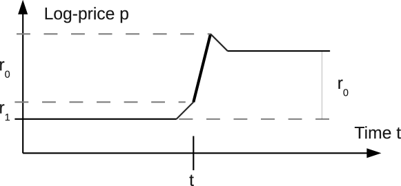
Figure 1: Price time dynamics around $t$ when trader 1 exploits his knowledge about $r_{0}$. This figure is readily generalised to the case of trader 1 and his friends exploiting $r_{0}$.

The paradox is the following: if trader $1$ is alone, the best return that can be extracted from his perfect knowledge is $\hat{g}_{1}(n_{1}^{*})$ according to the above reasoning. When there are $N$ traders in the ring of trust, the total return extracted is $N$ times the optimal gain of a single trader. Now, assume that trader $1$ has two brokering accounts; he can use each of his accounts, respecting the order in which to open and close his positions, effectively earning the optimal return on each of his accounts. The paradox is that his actions would be completely equivalent to investing $n_{1}^{*}$ and then $n_{1}^{*}$ from the same account. In particular, in the case of $I(n)=n$, this seems a priori exactly similar to grouping the two transactions into $2n_{1}^{*}$, but this results of course in a return smaller than the optimal return for a doubled investment. Hence, in this framework, trader $1$ can earn as much as pleases provided that he splits his investment into sub-parts of $n_{1}^{*}$ shares whatever $I$ is, as long as it is constant.

Two criticisms can be raised. First, the ring of trust must be perfect for this scheme to work, otherwise a Prisoner’s dilemma arises, as it is advantageous for trader $i+1$ to defect and close his position before trader $i$. In that case, the expected return for each trader is of order $1/N$, as in FarmerForce.

But more importantly, one may expect that the above discussion relies crucially on the fact that $r_{0}$ does not depend on the actual price, or equivalently that trader $0$ wishes to buy or to sell a predetermined number of shares. As we shall see in the second part of this paper, the paradox still exists even if trader $0$ has a fixed budget $C$ (which is more likely to arise if trader $0$ intends to buy).

But this paradox seems too good to be present in real markets. As a consequence, one should rather consider its impossibility as an a contrario consistency criterion for price impact functions. The final part of this paper explores the dynamics of price impact functions and the role of the spread in ensuring consistency, which is then tested in real markets.

3 Finite capital

When trader $0$ has a finite capital, the number of shares that he can buy decreases when traders $1$, $2$, …increase the share price before his transaction. Let us assume that trader $0$ has capital $C$ that buys $n_{0}$ shares at price $e^{p_{0}}$. The price he obtains is different from $e^{p_{0}}$ because of his impact: the real quantity of shares that $C$ can buy is therefore self-consistently determined by

$$n_{0}^{(0)}=\frac{n_{0}}{e^{I(n_{0}^{(0)})}}.$$ (4)

We shall first focus on the case where the self impact is neglected, or equivalently where trader $0$ has a restricted budget with flexible constraint since it is leads to simpler mathematical expressions.

When only trader $1$ is active before trader $0$, $n_{0}$ becomes $n_{0}^{(1)}=n_{0}/e^{I(n_{1})}$, thus the gain of trader $1$ is

$$g_{1}/e^{p_{0}}=n_{1}[e^{I(n_{0}/e^{I(n_{1})})}-e^{I(n_{1})}].$$ (5)

It is easy to convince oneself that there is always an $n_{1}^{*}\geq 1$ provided that $n_{0}$ is large enough: solving $\partial g_{1}/\partial n_{1}=0$ and setting $n_{1}=1$ gives the corresponding $n_{0}$. Using the shortcut $\rho=e^{I(1)}$,

$$e^{I(n_{0}/\rho)}\left[1-\frac{n_{0}}{\rho^{2}}I^{\prime}(1)I^{\prime}(n0/\rho)\right]-\rho[1+I^{\prime}(1)]=0$$ (6)

The existence of a solution to this equation is intuitive: when $n_{0}=0$, the left hand side is negative; since the second l.h.s term does not depend on $n_{0}$, one is left to show that the first l.h.s term grows fast enough with $n_{0}$ so that its parenthesis does vanish. Since $I^{\prime}(x)$ is assumed to be small in financial markets, the second l.h.s term is close to 1. Now, assuming that $I(x)$ grows at least as fast as a $\log x$, the first term always gives a solution. The case $I(x)\propto\log x$ is dealt with explicitly in the next subsection. At the other end of the spectrum of usual price impact functions, the linear case $I(x)=\lambda x$ cannot be solved exactly, but assuming that $\lambda\ll 1$ and perusing $e^{I(x)}\simeq 1+\lambda x$, one finds $n_{0}\simeq\frac{1+\lambda}{2\lambda^{2}}$, which deviates by about 3% from the numerical solution for $\lambda=0.01$.

Trader $1$ must now be careful when communicating the existence of the arbitrage to trader $2$, since the latter decreases the price return caused by trader $0$. Indeed, assuming that trader $1$ invests $n_{1}^{*}$ whatever trader $2$ does, his gain is given by

$$g_{1,2}(n_{1}^{*},n_{2})/e^{p_{0}}=n_{1}^{*}[e^{I(n_{2})+I(n_{0}/e^{I(n_{1}^{*})+I(n_{2})})}-e^{I(n_{2})+I(n_{1}^{*})}].$$ (7)

He would therefore lose $\Delta g_{1}(n_{2})=g_{1}^{*}-g_{1,2}(n_{1}^{*},n_{2})$, which must be compensated for by trader $2$. Without compensation payment, the gain of the latter is

$$g_{2}/e^{p_{0}}=n_{2}[e^{I(n_{0}/e^{I(n_{1}^{*})+I(n_{2})})}-e^{I(n_{2})}].$$ (8)

The case where trader $0$ has a strict budget constraint is obtained by replacing $n_{0}$ by $n_{0}^{(0)}$ in Eqs (5), (7) and (8).

The paradox exists if trader $2$ has a positive total gain, i.e., $G_{2}=g_{2}-\Delta g_{1}>0$. In order to investigate when this is the case, one must resort to particular examples of price impact functions.

Empirical research showed that $I$ is a non-linear, concave function [Hasbrouck91, KempfKorn99, FarmerImpact, BouchaudLimit2, RosenowImpact]. Although there is no consensus on its shape, logarithms and power- laws are possible candidates. From a mathematical point of view, logarithmic functions allow for explicit computations, while power-laws must be investigated numerically.

3.1 Log price impact functions

The generic impact function that will be studied is $I(|x|)=\rm{sign}(x)\gamma\log|\lambda x|$; when $\lambda>1$, a transaction of one share results in a price change; the number of shares will be rescaled so as to contain $\lambda$, which shorten the mathematical expressions. The parameter $\gamma\ll 1$ is related to the liquidity and brings down the impact to reasonable levels: if $x=100$ and $\gamma=0.01$, the price is increased by about $5$%.

For the sake of comparison, we first address the case of infinite capital: the optimal number of shares to invest by traders $1$ and $2$ is

$$n_{1}^{*}=\frac{n_{0}}{(\gamma+1)^{1/\gamma}},$$ (9)

which simplifies to $n_{0}/2$ if $\gamma=1$, and tends to $n_{0}/e^{1+\gamma/2}$ in the limit of small $\gamma$. The optimal monetary gain is given by

$$g_{1}^{*}=e^{p_{0}}n_{0}^{\gamma+1}\frac{\gamma}{(\gamma+1)^{1+1/\gamma}}.$$ (10)

In the case of finite capital, the optimal number of shares to invest for trader $1$ is

$$n_{1}^{*}=\left[n_{0}^{\gamma}(1-\gamma)\right]^{\frac{1}{\gamma(\gamma+1)}};$$ (11)

The optimal gain is given by

$$g_{1}^{*}=e^{p_{0}}n_{0}\frac{\gamma}{(1-\gamma)^{1-1/\gamma}}=C\frac{\gamma}{(1-\gamma)^{1-1/\gamma}},$$ (12)

which is linear in $n_{0}$, in contrast to its super-linearity in Eq (10): the limited budget of trader $0$ helps to remove predictability.

The gain of trader $1$ in the presence of trader $2$ is

$$g_{1,2}(n_{1}^{*},n_{2})=e^{p_{0}}n_{0}(1-\gamma)^{1/\gamma}\left(\frac{1}{(1-\gamma)n_{2}^{\gamma^{2}}}-1\right);$$ (13)

he therefore would lose

$$\Delta g_{1}(n_{2})=g_{1}^{*}-g_{1,2}(n_{1}^{*},n_{2})=e^{p_{0}}n_{0}(1-\gamma)^{1/\gamma-1}\left[1-\frac{1}{n_{2}^{\gamma^{2}}}\right].$$ (14)

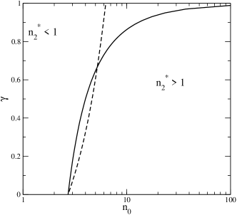
Figure 2: Region where the paradox exists ($n_{2}^{*}>1$) in parameter space ($n0$, $\gamma$). Logarithmic impact, finite capital with flexible constraint (continuous line) and strict constraint (dashed line).

Trader $2$ optimises

$$\frac{G_{2}}{e^{p_{0}}}=[g_{2}-\Delta g_{1}]e^{-p_{0}}=\left[\frac{n_{0}}{1-\gamma}\right]^{\frac{\gamma}{(\gamma+1)}}n_{2}^{1-\gamma^{2}}-n_{2}^{1+\gamma}-\Delta g_{1}(n_{2})$$ (15)

with respect to $n_{2}$. The paradox survives in the regions of the parameter space such that $G_{2}>0^{*}$ and $n_{2}^{*}>1$. Numerical investigations show that $G_{2}^{*}>0$ is always true. From Fig. 2 one sees that the paradox exists provided that scaled $n_{0}$ is large enough ($\lambda n_{0}>e^{1+\gamma/2}$ for $\gamma\ll 1$) and $\gamma$ small enough, which is compatible with all realistic values. Note that $g_{1}^{*}$ and $G_{2}^{*}$ are increasing functions of $\gamma$, since this parameter tunes the price return caused by $n_{0}^{(1)}$ and $n_{0}^{(2)}$.

If trader $0$ has a strict budget, the number of shares he can afford is determined self-consistently by $n_{0}^{(0)}=C/e^{p_{0}+\gamma\log n_{0}^{(0)}}$ without the intervention of the trader $1$, that is, $n_{0}^{(0)}=n_{0}^{1/(\gamma+1)}$; after trader $1$ has opened his position, trader $0$ can only afford

$$n_{0}^{(1)}=n_{0}^{(0)}/n_{1}^{\gamma/(\gamma+1)}=\left[\frac{n_{0}}{n_{1}^{\gamma}}\right]^{\frac{1}{\gamma+1}}$$ (16)

shares. Similarly,

$$n_{1}^{*}=n_{0}^{\frac{1}{2\gamma+1}}\left[\frac{1-\gamma^{2}/(\gamma+1)}{\gamma+1}\right]^{\frac{\gamma+1}{\gamma(2\gamma+1)}},$$ (17)

hence the number of shares to invest is lowered further in comparison with Eq (11). All the expressions of the respective gains of trader $1$ and $2$ do not simplify to neat and short expressions and no analytical solution to the maximisation of $G_{2}$ can be found. Numerical maximisation yields the dashed boundary line in Fig. 2. The strict constraint increases the minimum $n_{0}$ needed for making the paradox possible when $\gamma$ is small enough. At $\gamma\simeq 0.66$, the boundary lines cross; this may be due to the fact that trader $2$ must pay a smaller compensation to trader $1$ when $\gamma$ increases.

3.2 Power-law impact functions

Several papers suggest a power-law price impact function $I(x)=\rm{sign}x|x/\lambda|^{\beta}$ with $\lambda\geq 1$ and $\beta\in[0.3,0.8]$ [StanleyImpact, RosenowImpact, FarmerImpact]; for the sake of simplicity (and without loss of generality) the volumes $x$ will be rescaled by $\lambda$ from now on; this means that the consistency conditions are now $G_{2}>0$ and $n_{2}>0$. With this choice of functions, it is not possible to maximise explicitly $g_{1}$ and $G_{2}$.

Figure 3: Region where the optimal gain of trader $2$ is positive in the (scaled) $n_{0}$, $\beta$ space. Power-law impact function and finite capital.

Performing all the maximisations of the finite capital case numerically, one finds that the picture of the $\log$ impact function is still valid in this case (see Fig. 3): realistic values of (scaled) $n_{0}$ are small, hence they always fall into the region of inconsistency, in particular for $I(x)\propto x$. Interestingly, this is the most common choice in the literature on agent-based models, option pricing, etc. It was derived analytically by Kyle85 under the assumption of linearity between private information and insiders’ order flow. More recently, FarmerForce uses it as simple example of a function that prevents making trading profits from a round trip. And certainly, it may seem the least arbitrary, since it does not seem to impose any particular choice of $\beta$. Hence constant $I(x)\propto x$ is to be banished. But power-laws are inconsistent for all possible real-market values of $\beta$; once again, this shows that constant price impact functions are to be avoided.

4 Feedback

A possible way out from inconsistent price impact functions is to take into account the dynamics of the order book, particularly the reaction of the order book to a sequence of market orders of the same kind. Generically, the impact of a second market order of the same kind and size is smaller than that of the first one, and similarly for a third one. For our purpose, we shall assume that a second market order of the same size and type has an impact described by $I_{1}(n)=\kappa_{1}I(n)$ with $0<\kappa_{1}<1$, the third $I_{2}(n)=\kappa_{2}\kappa_{1}I(n)$, etc [BouchaudLimit5, FarmerMolasses]. To this contraction of market impact on one side also corresponds an increase of market impact on the other side for the next market order of opposite type [BouchaudLimit5]; therefore, we shall assume that the impact function on the other side is divided by $\theta_{1}$ after the first market order, by $\theta_{2}\theta_{1}$ after the second, etc. As shown in the next section, $\kappa_{1}\simeq\kappa_{2}$ is a very good approximation when $\kappa_{1}$ and $\kappa_{2}$ are averaged over all the stocks, hence we shall assume $\kappa_{1}=\kappa_{2}=\kappa$; for the same reason, we assume that $\theta_{1}=\theta_{2}=\theta$. The hypothesis that the contractions of the price impact functions correspond to multiplying $I$ for each new market order makes this process Markovian. While it is now well established that order books and order flows are not Markovian but display long memory [FarmerMolasses, BouchaudImpact2], this may seem a step back. However since we only consider a few time steps, the long memory of the order book is of little importance for the present discussion.

When writing the gains of trader $1$ and $2$, one must be very careful with the order of the transactions. Starting with the case of infinite capital of trader $0$, the gain of trader $1$ is

$$g_{1}=n_{1}[e^{I(n_{1})+\kappa I(n_{0})-I(n_{1})/\theta^{2}}-e^{I(n_{1})}],$$ (18)

which makes it clear that there is still a non-zero optimal number of shares $n_{1}^{*}$ to invest. Similarly, the gain $g_{1,2}$ is now

$$g_{1,2}=n_{1}^{*}[e^{I(n_{2})+\kappa I(n_{1}^{*})+{\kappa^{2}}I(n_{0})-I(n_{1}^{*})/\theta^{3}}-e^{I(n_{2})+\kappa I(n_{1}^{*})}],$$ (19)

while that of trader 2, without his payment to trader 1 is

$$g_{2}=n_{2}(e^{I(n_{2})+\kappa I(n_{1}^{*})+{\kappa^{2}}I(n_{0})-I(n_{1}^{*})/\theta^{3}-\kappa I(n_{2})/\theta^{2}}-e^{I(n_{2})}).$$ (20)

4.1 Feedback on market order side only

In order to investigate whether the feedback on the side on which the first sequential market orders are placed is enough to make price impact consistent, one sets $\theta=1$. In the case of $\log$ price impact functions, the optimal number of shares and gain of trader $1$ are

$$n_{1}^{*}=\frac{n_{0}^{\kappa}}{(\gamma+1)^{1/\gamma}}$$ (21)

and

$$g_{1}^{*}=e^{p_{0}}n_{0}^{\kappa(\gamma+1)}\frac{\gamma}{(\gamma+1)^{1+1/\gamma}}.$$ (22)

These two equations already show that the reaction of the limit order book reduces the gain opportunity of player $1$. Adding trader $2$ will reduce further the impact of trader $0$, hence the gain of trader $1$, and, as before, trader $2$ should pay for it. In this case, the reduction of gain of trader $1$ is

$$\frac{\Delta g_{1}}{e^{p_{0}}} = [g_{1}^{*}-g_{1}(n_{1}^{*},n_{2})]e^{-p_{0}}=n_{0}^{\kappa(\gamma+1)}\frac{\gamma}{(\gamma+1)^{1+1/\gamma}}$$ (23)

$$-n_{2}^{\gamma}\frac{n_{0}^{\gamma(1+\kappa\gamma)}}{(\gamma+1)^{1/\gamma+\kappa}}[n_{0}^{-\gamma\kappa(1-\kappa)}(\gamma+1)-1],$$

while the gain that trader $2$ optimises is

$$\frac{G_{2}}{e^{p_{0}}}=n_{2}^{\gamma+1}\left[\frac{1}{n_{2}^{\kappa\gamma}}\frac{n_{0}^{\kappa\gamma(2\kappa-1)}}{(1+\gamma)^{\kappa-1}}-1\right]-\frac{\Delta g_{1}}{e^{p_{0}}}.$$ (24)

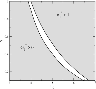
Figure 4: Regions in which the optimal gain of trader $2$ is positive and in which the number of shares invested by trader $1$ is larger than $1$. Logarithmic impact, infinite capital, and feedback on market orders side only ($\kappa=0.5$).

Trader $1$’s impact functions are $\kappa I$ when he opens his position and $I$ when he closes it, which is an additional cause of loss for trader $1$, which must be also compensated for by trader $2$. Fortunately for the latter, his impact functions are $I$ when opening and $\kappa I$ when closing his position. Therefore, provided that $\kappa$ is large enough so as not to make the impact of the trader 0 $\kappa^{2}I(n_{0})$ too small, trader $2$ can earn more than trader $1$ in some circumstances.

As above, impact functions are inconsistent when $G_{2}^{*}>0$, $n_{1}^{*}>1$ and $n_{2}^{*}>1$ for $\log$ impact functions. It turns out that the regions in which $G_{2}^{*}>0$ while $n_{1}^{*}>1$ are disjoint if $\kappa<\kappa_{c}\simeq 0.5$ for $\log$ impact functions (Fig. 4).

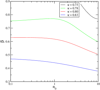
Figure 5: Regions of parameter space where the optimal gain of trader $2$ ($G_{2}^{*}$) is positive (above the respective line). Power-law impact functions, feedback with infinite capital. From top to bottom $\kappa=0.75$, $0.78$, $0.8$ and $0.83$.

The case of power-law impact functions shows a similar transition: since $n_{0}$ is rescaled, the realistic region to consider is limited to $n_{0}\ll 1$, for which the region $G_{2}^{*}>0$ vanishes when $\kappa<\kappa_{c}\simeq 0.78$ (Fig. 5).

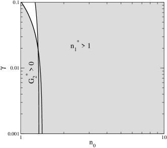
Figure 6: Regions in which the optimal gain of trader $2$ is positive and in which the number of shares invested by trader $1$ is larger than $1$. Logarithmic impact, infinite capital, and feedback on both sides ($\kappa=0.83$)

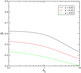
Figure 7: Regions in which the optimal gain of trader $2$ is positive (above the respective line). Power-law impact, infinite capital, and feedback on both sides; from top to bottom: $\kappa=0.91$ (black line), $\kappa=0.92$ (red line), $\kappa=0.93$ (green line).

4.2 Feedback on both sides

We shall assume that $\theta_{1}=\theta_{2}=\kappa$ in order to be able to use market data. Generalising the above calculations is straightforward. As an example, for $\log$ price impact functions,

$$n_{1}^{*}=n_{0}^{\kappa^{3}}\left[\frac{1-\gamma(1/\kappa^{2}-1)}{1+\gamma}\right]^{\kappa^{2}/\gamma}.$$ (25)

Once again, more feedback results in a smaller exponent of $n_{0}$. As a consequence, Fig. 6 shows that the critical value of $\kappa$ is slightly larger than $0.83$ for $\log$ price impact functions all $\gamma$: indeed only a small area of inconsistent impact functions, corresponding to $n_{0}\simeq 1.5$, still exists but cannot be reached since both $n_{0}=1$ and $2$ are outside of the inconsistent region. The effect of feedback on power-law price impact functions is stronger (see Fig. 7): when $\kappa<0.92$, (scaled), only power-laws with exponent larger than about $0.5$ (this includes linear and super-linear impact functions) are inconsistent for reasonable values of $n_{0}$. Therefore, even double feedback does not guarantee consistency

5 Empirical data

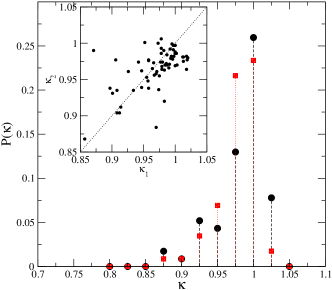
Figure 8: Empirical distribution of $\kappa_{1}$ (black circles) and $\kappa_{2}$ (red squares) of 68 stocks of Paris Stock Exchange in 2002. Inset: $\kappa_{2}$ vs $\kappa_{1}$ for all the stocks

The values of $\kappa_{1}$ and $\kappa_{2}$ can be measured in real markets. The response function $R(\delta t,V)=\langle{(p(t+\delta t)-p(t))\epsilon(t)|V(t)=V}\rangle$ is the average mid-price change after $\delta t$ trades, conditional on the sign of the trade $\epsilon(t)$ and on volume $V$; similarly, one defines the response function conditional on two trades of the same sign $R^{+}(\delta t,V)=\langle{(p(t+\delta t)-p(t))\epsilon(t)|V(t)=V,\epsilon(t)=\epsilon(t-1)}\rangle$, and $R^{++}(\delta t,V)=\langle{(p(t+\delta t)-p(t))\epsilon(t)|V(t)=V,\epsilon(t)=\epsilon(t-1)=\epsilon(t-2)}\rangle$. A key finding of BouchaudLimit3 and BouchaudLimit4 is that $R$ factorises into $R(\delta t)F(V)$. Thus we will be interested in $R(\delta t)$, $R^{+}(\delta t)$ and $R^{++}(\delta t)$.

Using measures kindly provided by J.-Ph. Bouchaud and J. Kockelkoren taken on one year of data about all the order books of Paris Stock Exchange, one finds that the estimate $\hat{\kappa}$ of $\kappa$, defined as $\hat{\kappa}=\langle{R^{+}(1)}\rangle/\langle{R(1)}\rangle\in[0.86,1.02]$, that the average over all stocks $\overline{\hat{\kappa}_{1}}=0.97\pm 0.04$ and $\hat{\kappa}_{2}=\langle{R^{++}(1)}\rangle/\langle{R^{+}(1)}\rangle\in[0.87,1.01]$, while $\overline{\hat{\kappa}_{2}}=0.97\pm 0.03$. (see Fig. 8); for a given stock, there is some correlation between $\kappa_{1}$ and $\kappa_{2}$ (see inset of Fig. 8); the data presented here does not contain error bars for the measures of $R$, $R^{+}$ and $R^{++}$. The approximation $\kappa_{1}\simeq\kappa_{2}$ is reasonable, and we shall from now on call $\kappa=(\kappa_{1}+\kappa_{2})/2$ and replace $\kappa_{1}$ and $\kappa_{2}$ by $\kappa$ everywhere. It should be noted that since one considers the mid-price reaction to a market order, in principle, the measured values of $R$, $R^{+}$, and $R^{++}$ include the spread. However, because $\kappa$ is the ratio between two of them, this effect cancels out.

In other words there is some variations between the stocks, some of them being less sensitive to successive market orders of the same kind. The values of estimated $\kappa$ start at $0.86$. Therefore, even feedback on both book sides does not yield consistent $\log$ impact functions, but do if the impact functions are power-laws with small exponents. One concludes that the feedback of the order book is not enough to make price impact functions consistent.

6 Spread without feedback, infinite capital

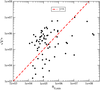
Figure 9: Average daily volume versus $n_{0,min}$ (same data set)

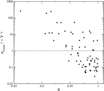
Figure 10: Fraction of daily volume needed to inject an exploitable arbitrage versus $\kappa$ (same data set)

The above discussion neglects the bid-ask spread $s$. It is however of great importance in practice, as the impact of one trade is on average of the same order of magnitude as the spread [BouchaudLimit5]. This means that $n_{0}$ must be large enough in order to make the knowledge of trader $1$ valuable. Assuming that the spread is equal to $\langle{s}\rangle$ at all times, Eq. (5) generalises to

$$\frac{g_{1}}{e^{p_{0}}}=n_{1}\left[e^{I(n_{0})-\langle{s}\rangle}-e^{I(n_{1})}\right].$$ (26)

Thus, replacing $n_{0}$ by $n_{0}^{\prime}=I^{-1}[I(n_{0})+\langle{s}\rangle]$ leads to the same equations as before. For example, in the case of $log$ impact functions, $n_{0}^{\prime}=n_{0}e^{-\frac{\langle{s}\rangle}{\gamma}}$ and the optimal number of shares that trader $1$ should invest is

$$n_{1,s}^{*}=\frac{n_{0}e^{-\langle{s}\rangle/\gamma}}{(1+\gamma)^{1/\gamma}}$$ (27)

and his optimal gain is given multiplied by $e^{-\frac{1+\gamma}{\gamma}\langle{s}\rangle}\simeq e^{-\frac{\langle{s}\rangle}{\gamma}}$. Since $\langle{s}\rangle/\gamma\sim 10$ in practice, the minimal amount of shares needed to create an arbitrage, denoted by $n_{0,\min}$ is increased (and his gain divided) about 20,000 folds by the spread. Straightforward calculations show that replacing $n_{0}$ by $n_{0}^{\prime}$ holds for all the equations investigated in previous subsections.

The respective values of $\gamma$ and $\langle{s}\rangle$ are not independent, and can be measured in real markets for a given stock. In the language of BouchaudLimit3, $\gamma=\langle{\log(n)}\rangle/R(1)$ where $\langle{\log(n)}\rangle$ is the average of the logarithm of transaction size and $R(1)$ is the response function after one time step. Using $\gamma$ and $\langle{s}\rangle$ measured in Paris Stock Exchange one finds that $n_{0,\min}\in[1.210^{4},2.010^{8}]$, with median of $1.210^{5}$ (Fig. 9), which is not irrealistic for very liquid stocks. Indeed, the fraction of $n_{0,\min}$ with respect to the average daily volume of each stock ranges from $\simeq 2\%$ to more than $100\%$, with a median of about $42\%$. Therefore, for most of the stocks, trader $0$ needs to trade less than two fifths of the daily average volume in one transaction in order to be leave an exploitable arbitrage; for 12 stocks ($18\%$), trading less than $10\%$ of the average daily volume suffices. It is unlikely that a single trade is larger than the average daily volume, hence, 29 stocks ($43\%$) do not allow on average a single large trade to be exploitable by a simple round-trip. Interestingly, stocks with average daily volumes smaller than about $10^{5}$ are all consistent from that point of view (Fig. 9). In addition, the stocks for which $n_{0,\min}<\langle{V}\rangle$ all have a $\kappa>0.945$.

Therefore, the role of the spread is to increase considerably the minimum size of the trade, which in some cases remain within reasonable bounds. Therefore, the spread must be taken into account, but does not yield systematically consistent impact functions for some stocks with a high enough daily volume.

7 Spread and feedback, infinite capital

The question is whether the feedback and the spread make impact function systematically consistent. The stocks that are the most likely to become consistent are those whose $n_{0,\min}/\langle{V}\rangle<1$ is large while having a strong feedback. According to Fig. 10, these properties are compatible.

Using for each stock $\langle{s}\rangle$, $\kappa$, and $\gamma$ from the data, we find that three additional stocks (ALS, IFG, SCO) are made consistent by feedback on trader $0$’s market order side alone: the feedback limited to one side of the order book, even when the spread is taken into account, is insufficient. However, adding finally the feedback on both book sides makes consistent all the stocks, even in the case of infinite capital. Therefore, both the spread and the feedback on both sides of the order book are crucial ingredients of consistency at the smallest time scale.

8 Discussion

The paradox proposed in this paper provides an a contrario simple and necessary condition of consistency for price impact functions. This condition is verified for all the stocks of Paris Stock Exchange in 2002. Indeed, the main finding of this paper is that financial markets ensure consistent market price impact functions on average at the most microscopic dynamical level by two essential ingredients: the spread and the dynamics of the order book on both sides of the order book.

The fact that non-constant price impact functions with feedback are needed to achieve consistency at the smallest time scale for more than half of the stocks means that financial literature that assumes constant price impact functions must be critically reviewed in this light. This paper is not the first to suggest it (see e.g [BouchaudLimit3, BouchaudLimit4, FarmerImpact, FarmerMolasses]), but advocates it from logical evidence: for instance HubermanStanzl shows that if the price impact is permanent, only linear impact functions prevent quasi-arbitrage, but recognises the paradox that real-market price impact functions are not linear, therefore suspects the need for time-dependent impact functions. The approach of the present paper remains Markovian, which is justified when restricting one’s attention to the smallest time scale and a few transactions only. However, in general, the long memory of the side of limit order markets must be compensated in a subtle way by the price impact functions (see e.g. BouchaudLimit4 and FarmerMolasses). This raises the crucial issue of how to incorporate in a tractable way non-constant impacts in microstructure and agent-based modelling.

I am indebted to Jean-Philippe Bouchaud, Julien Kockelkoren and Michele Vettorazzo from CFM for their hospitality, measurements, and comments. It is a pleasure to acknowledge discussions and comments from Doyne Farmer, Sam Howison, Matteo Marsili, Sorin Solomon and David Brée, and useful criticisms by an anonymous referee.

References

- [1] \harvarditemBachelier1900bachelier Bachelier, L.: 1900, Théorie de la Spéculation, Vol. 3 of Annales Scientifiques de l’Ecole Normale Superieure, pp. 21–86.
- [2] \harvarditemBouchaud, Gefen, Potters and Wyart2004BouchaudLimit3 Bouchaud, J.-P., Gefen, Y., Potters, M. and Wyart, M.: 2004, Fluctuations and response in financial markets: the subtle nature of ‘random’ price changes, Quant. Fin. 4, 176.
- [3] \harvarditemBouchaud, Kockelkoren and Potters2004BouchaudImpact2 Bouchaud, J.-P., Kockelkoren, J. and Potters, M.: 2004, Random walks, liquidity molasses and critical response in financial markets, Quant. Fin. 6, 115–123. cond-mat/0406224.
- [4] \harvarditem[Bouchaud et al.]Bouchaud, Kockelkoren and Potters2006BouchaudLimit4 Bouchaud, J. P., Kockelkoren, J. and Potters, M.: 2006, Random walks, liquidity molasses and critical response in financial markets, Quant. Fin. 6, 115–123.
- [5] \harvarditemBouchaud and Potters2003BouchaudLimit2 Bouchaud, J.-P. and Potters, M.: 2003, More statistical properties of order books and price impact, Physica A 324, 133.
- [6] \harvarditemChallet2007C05 Challet, D.: 2007, Inter-pattern speculation: beyond minority, majority and $-games, J. Econ. Dyn. and Control. (32). physics/0502140.
- [7] \harvarditem[Challet et al.]Challet, Marsili and Zhang2000MMM Challet, D., Marsili, M. and Zhang, Y.-C.: 2000, Modeling market mechanisms with minority game, Physica A 276, 284. cond-mat/9909265.
- [8] \harvarditem[Chen et al.]Chen, Stanzl and Watanabe2002ChenLimitArbitrage Chen, Z., Stanzl, W. and Watanabe, M.: 2002, Price impact costs and the limit of arbitrage. Yale ICF Working Paper No. 00-66.
- [9] \harvarditemFama1970Fama Fama, E. F.: 1970, Efficient capital markets: a review of theory and empirical work, J. of Fin. 25, 383–417.
- [10] \harvarditemFarmer1999FarmerForce Farmer, J. D.: 1999, Market force, ecology and evolution, Technical Report 98-12-117, Santa Fe Institute.
- [11] \harvarditem[Farmer et al.]Farmer, Gerig, Lillo and Mike2007FarmerMolasses Farmer, J. D., Gerig, A., Lillo, F. and Mike, S.: 2007, Market efficiency and the long-memory of supply and demand: Is price impact variable and permanent or fixed and temporary?
- [12] \harvarditemGatheral2009gatheral-no Gatheral, J.: 2009, No-dynamic-arbitrage and market impact, Quant. Fin. . to appear.
- [13] \harvarditemHasbrouck1991Hasbrouck91 Hasbrouck, J.: 1991, Measuring the information content of stock trades, J. of Finance 46, 179–207.
- [14] \harvarditemHuberman and Stanzl2004HubermanStanzl Huberman, G. and Stanzl, W.: 2004, Price manipulation and quasi-arbitrage, Econometrica, 72, 1247–1275.
- [15] \harvarditemHull2005HullBook Hull, J. C.: 2005, Options, Futures And Other Derivatives, Prentice Hall.
- [16] \harvarditemKempf and Korn1992KempfKorn99 Kempf, A. and Korn, O.: 1992, Market depth and order size, J. of Fin. Markets 2, 29–48.
- [17] \harvarditemKyle1985Kyle85 Kyle, A. S.: 1985, Continuous auctions and insider trading, Econometrica 53, 1315–1335.
- [18] \harvarditemLillo and Farmer2004FarmerSign Lillo, F. and Farmer, J. D.: 2004, The long memory of efficient markets, Non-lin. Dyn. and Econometric 8.
- [19] \harvarditem[Lillo et al.]Lillo, Farmer and Mantegna2003FarmerImpact Lillo, F., Farmer, J. D. and Mantegna, R.: 2003, Econophysics - master curve for price - impact function., Nature 421, 129.
- [20] \harvarditem[Madhavan et al.]Madhavan, Richardson and Roomans1997Madhavan Madhavan, A., Richardson, M. and Roomans, M.: 1997, Why do security prices fluctuate? a transaction-level analysis of nyse stocks, Review of Financial Studies 10, 1035.
- [21] \harvarditem[Plerou et al.]Plerou, Gopikrishnan, Gabaix and Stanley2004StanleyImpact Plerou, V., Gopikrishnan, P., Gabaix, X. and Stanley, H. E.: 2004, On the origin of power-law fluctuations in stock prices, Quant. Fin. 4, C11–C15.
- [22] \harvarditemRosenow2005RosenowImpact Rosenow, B.: 2005, Order book approach to price impact, Quant. Fin. 5, 357 – 364.
- [23] \harvarditemThaler2005BehavioralFinance Thaler, R. H. (ed.): 2005, Advances in behavioral finance, Princeton University Press, Princeton.
- [24] \harvarditem[Wyart et al.]Wyart, Bouchaud, Kockelkoren, Potters and Vettorazzo2006BouchaudLimit5 Wyart, M., Bouchaud, J.-P., Kockelkoren, J., Potters, M. and Vettorazzo, M.: 2006, Relation between bid-ask spread, impact and volatility in double auction markets.
- [25]