Oscillation and levitation of balls
in continuously stratified fluids

Abstract

The free motion of balls is investigated experimentally in continously stratified fluid in a finite container. The oscillation frequency is found to be very close to the local Brunt–Väisäla frequency. The effect of added mass proves to be practically negligible. The evolution of rear jets is demonstrated, and a kind of long term levitation is found. We show that the classical viscous drag would lead to a much stronger damping than observed in the experiment. This is interpreted as a consequence of the feedback from the previously excited internal waves following their reflection from the boundaries. A phenomenological equation with a modified drag term is proposed to obtain a qualitative agreement with the observations. We point out that the inclusion of a history term would lead further away from the observed data.

1 Introduction

The motion of a spherical body in a fluid is one of the historical and still open problems of physics. Its research dates back to the 18th century, continuing with the works of Poisson, Green, Stokes and other outstanding scientists of the 19th century, including the derivation of the famous history force by Boussinesq [1] in 1885 (and, apparently independently, by Basset [2] three years later). The correct mathematical formulation of these two nontrivial effects had been the subject of research for about a century, before the equation of motion, valid at least for a small rigid sphere in an unbounded homogeneous fluid at low Reynolds numbers, was finally settled by the work of Maxey and Riley [3] (see also [4]). Their approach has lead to a series of experimental and theoretical investigation of finite particle motion in cases under more general conditions, as well (for reviews see [5, 6], for a few recent examples, see [7, 8] and [9], respectively).

An analogous problem is the motion of a rigid sphere in stably stratified fluid. In an early approach, before the publication of the Maxey–Riley equation, Larsen [10] pointed out the importance of the generation of internal waves and derived a linear equation for the oscillation of the sphere about its stable equilibrium in an inviscid fluid when damping is entirely due to wave radiation. More recently, the flow past a vertically moving ball has been studied experimentally and numerically [11, 12], and the appearance of a ’rear jet’ was pointed out, in which light fluid dragged down by the ball emerges from the boundary layer in a narrow column in the wake of the falling body. Investigations of the gravitational settling of particles through sharp density interfaces [13, 14] show that the light fluid surrounding the ball slows down the settling, and might even lead to a temporary rising, ’levitation’ [14], of the otherwise denser body.

A somewhat related approach is the study of internal wave generation by vibrating obstacles [15, 16, 17, 18]. For these forced types of motion the authors find in linear approximation that both the added mass and the viscous drag are frequency dependent, and their actual value does also depend on the ratio of the size of the moving body to the fluid depth.

In this paper we report upon our experimental investigation of the free motion of balls in continously stratified fluid in a finite container. The oscillation frequency of a fluid element is known to be given by the Brunt–Väisäla (BV) frequency. The ball’s frequency might, however, be different due to the added mass, history and other effects. The basic questions raised in the paper are

• is the oscillation frequency close to the BV frequency,

• is the damping primarily determined by the viscous drag,

• is an asymptotic state reached in the experiment,

• is there any equation which could faithfully describe the phenomenon?

We point our that in the course of the ball’s motion, viscosity, wave generation and the reflection of internal waves from the boundaries all play an important role.

In the next section different available forms of equations of motion are reviewed. Then (Sections 3,4) we describe the experimental set-up and data acquisition. In Section 5 we present shadow-graphs showing the evolution of rear jets during this nonmonotonic fall as well, and find a kind of long term levitation. Section 6 is devoted to the analysis of the oscillation frequency which proves to be very close to the local BV frequency. This implies that the effect of added mass is practically negligible during the late stage of the motion. In Section 7 we show that classical viscous drag would lead to a much stronger damping than observed in the experiment. We interpret this as a consequence of the feedback from the previously excited internal waves following their reflection from the boundaries, and apply a phenomenological equation with a modified drag term to obtain a qualitative agreement with the observations. The concluding section points out that the inclusion of a history term would lead further away from the observed data. A new term, whose explicit form remains unknown, is, however, needed in a correct equation of motion, a term which accounts for the fluid motion generated by the internal waves.

2 Theoretical background

In an infinite homogeneous fluid of density $\varrho_{f}$, the equation of motion of a small rigid spherical nonrotating particle of radius $r$ and mass $m_{p}$, starting from rest at $t=0$, is given by the Maxey–Riley equation  [3, 4]:

$$m_{p}\ddot{\mathbf{r}} = m_{f}\frac{D\mathbf{u}}{Dt}(\mathbf{r},t)+\frac{1}{2}m_{f}\left(\frac{D\mathbf{u}}{Dt}(\mathbf{r},t)-\ddot{\mathbf{r}}\right)+(m_{p}-m_{f})\mathbf{g}$$ (1)

$$-6\pi r\nu\varrho_{f}\left(\dot{\mathbf{r}}-\mathbf{u}(\mathbf{r},t)\right)+\mathbf{F}_{\mathrm{history}}(t),$$

where $\mathbf{r}(t)$ is the location of the particle at time $t$, $\mathbf{u}(\mathbf{r},t)$ is the undisturbed velocity field of the fluid in the absence of the ball (as determined by the boundary conditions and external sources), ${D\mathbf{u}}/{Dt}={\partial\mathbf{u}}/{\partial t}+(\mathbf{u}\cdot{\nabla})\mathbf{u}$ is the usual hydrodynamical time derivative of the velocity following a fluid element, $m_{f}$ is the mass of the fluid displaced by the sphere, and $\nu$ is the kinematic viscosity. The force terms on the right hand side represent the hydrodynamical force, the added mass contribution, the buoyancy corrected weight, the Stokes drag and the history term, respectively. The equation is valid for small relative velocities, when the history term takes the form

$$\mathbf{F}_{\mathrm{history}}(t)=-6r^{2}\varrho_{f}(\pi\nu)^{1/2}\int_{0}^{t}d\tau\,\frac{\ddot{\mathbf{r}}(\tau)-{d\mathbf{u}}(\mathbf{r}(\tau),\tau)/{d\tau}}{{(t-\tau)}^{1/2}}$$ (2)

where ${d\mathbf{u}}/{dt}={\partial\mathbf{u}}/{\partial t}+(\dot{\mathbf{r}}\cdot{\nabla})\mathbf{u}$ is the time derivative following the path of the particle. This term is due to the fact that the particle modifies the flow locally.

The original equation of Maxey and Riley [3, 4] contain further correction terms for strongly nonuniform background flows. These terms have been omitted from Eq. (1) for simplicity, since in what follows we consider only the case when the unperturbed fluid is at rest: $\mathbf{u}(\mathbf{r},t)\equiv 0$. We shall also assume that the motion takes place in the vertical direction, along the $z$ axis.

At large particle velocities the Stokes drag is replaced by the nonlinear drag

$$-c_{D}(Re)\frac{r^{2}\pi}{2}\varrho_{f}\left|{\dot{z}}\right|\dot{z}$$ (3)

where $c_{D}$ is the empirically known drag coefficient [19], a function of the instantaneous Reynolds number

$$Re=\frac{2r\left|{\dot{z}}\right|}{\nu}.$$ (4)

In this regime, the form of the history term is known to differ from (2), and it is doubtful that it can be expressed at all as a convolution with a simple kernel. In any case it appears to decay faster then in the Stokes regime (see e.g. [7]).

We extend Eqs. (1) and (2) to allow spatially varying fluid densities $\varrho_{f}(z)$ as follows

$$\ddot{z}=-\sigma\frac{\varrho_{f}(z)}{\varrho_{p}}\ddot{z}-\frac{\varrho_{p}-\varrho_{f}(z)}{\varrho_{p}}g-c_{D}(2r\left|{\dot{z}}\right|/\nu)\frac{3\varrho_{f}(z)}{8r\varrho_{p}}\left|{\dot{z}}\right|\dot{z}\,,$$ (5)

where $m_{p}=4\pi\varrho_{p}r^{3}/3$ has been used with $\varrho_{p}$ as the particle density. Since the coefficient of the added mass effect is not a unique constant in stratified flows, we replaced $1/2$ by an unknown coefficient $\sigma$. The history term has not been written out since its contribution is found to be negligible in our experiment. We shall return to a discussion of the relevance of this term in the Conclusions.

According to Eq. (5) the particle is in a stable equilibrium at the height where $\varrho_{f}(z)=\varrho_{p}$, which we choose as a convenient reference height $z=0$ in the following. Assuming small amplitude oscillation around this neutrally buoyant position, we can write $\varrho_{p}-\varrho_{f}(z)=z\varrho_{p}N^{2}/g$, where $N$ denotes the local Brunt–Väisäla (BV) frequency. If the amplitude is small enough, the velocity amplitude can also be small enough to ensure the Stokesian regime all the time, the drag coefficient is then $c_{D}(Re)=24/Re$ [20]. Thus we obtain

$$(1+\sigma)\ddot{z}=-N^{2}z-2\alpha_{0}\dot{z},$$ (6)

where

$$\alpha_{0}=9\nu/(4r^{2})$$ (7)

is a damping coefficient. The motion is then that of a linearly damped harmonic oscillator with frequency $\omega_{0}$, given by

$$\omega_{0}^{2}=\frac{N^{2}}{1+\sigma}-\frac{\alpha_{0}^{2}}{(1+\sigma)^{2}}.$$ (8)

It is remarkable that both viscosity and added mass effect tend to decrease the oscillation frequency below the BV value. An important dimensionless parameter of the problem is

$$St=\frac{\nu}{r^{2}N}=\frac{2Fr}{Re},$$ (9)

which can be considered as a Stokes number. $St$ is basically the ratio of the instantaneous Froude number,

$$Fr=\frac{\dot{z}}{Nr}$$ (10)

and the Reynolds number.

An alternative approach is due to Larsen [10] who derived for a small amplitude oscillations of a sphere, released initially at height $z(0)$:

$$\ddot{z}=-N^{2}z+\frac{z-z(0)}{t^{2}}-\frac{\dot{z}}{t}.$$ (11)

The last two terms on the right hand side express energy loss due to radiation of internal waves, an effect not taken into account in (5). This approach neglects, however, viscous effects. Due to the presence of the inhomogeneous terms, no clear oscillation frequency can be defined for short times.

At present, no equation is known which would be able to account for nonlinear internal wave generation during the ball’s motion.

3 Experimental setup and density profiles

The experiments were carried out in a glass tank of size $75\;\mathrm{cm}\times 38\;\mathrm{cm}\times 50\;\mathrm{cm}$. The salt density stratification was produced by a double-bucket equipment [21]. A typical water height of 38 – 39 cm was used.

The ambient density profile $\varrho_{f}(z)$ was obtained by measuring the conductivity and the temperature of the salt solution at different heights $z$, and by extracting the density values from tabulated data.

The average BV frequency, $\bar{N}$, was deduced from the average slope of the density profile. Table 1 indicates these frequencies in the five different profiles used.

Profile	$\overline{N}$ (1/s)
1	$1.21\pm 0.02$
2	$1.23\pm 0.02$
3	$0.86\pm 0.01$
4	$0.58\pm 0.01$
5	$1.12\pm 0.03$

Table 1: The average BV frequency for the different density profiles used.

A careful investigation of the profiles indicated that there was a slight static deviation superimposed on the linear slope. In order to obtain a more precise expression for the local BV frequency, $N(z)$, at different heights, we fitted a cubic polynomial to the density data, which proved to be an appropriate form for all the profiles. A typical profile and the fitted polynomial is shown in Fig. 1.

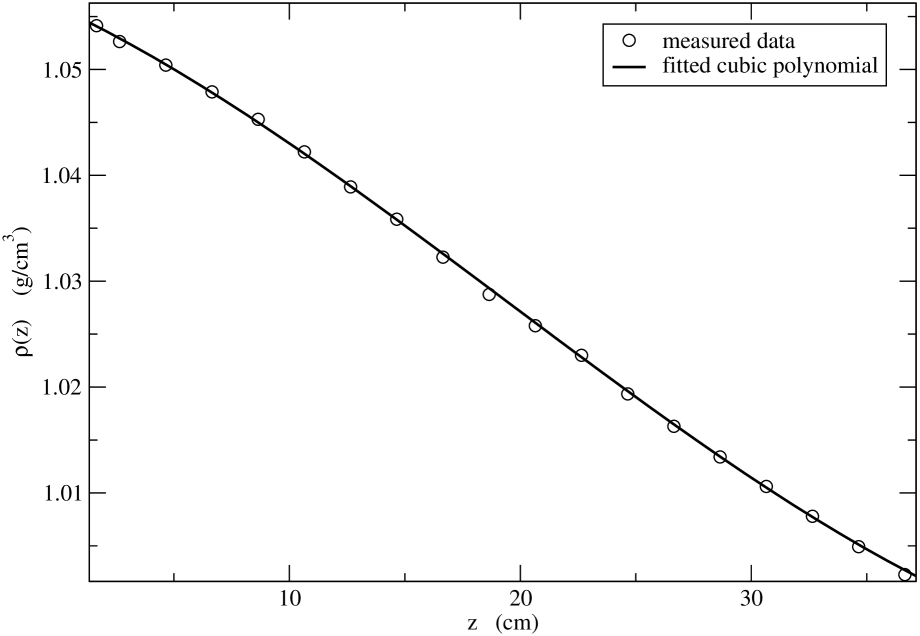
Figure 1: The density profile no. 1 (cf. Table 1). The cubic polynomial fitted to the data is $\varrho_{f}(z)=1.0559-1.02\times 10^{-3}z-3.14\times 10^{-5}z^{2}+5.39\times 10^{-7}z^{3}$, where density and height are measured in g/cm³ and cm, respectively.

The motion of five different balls of radius $r=7.3\;\textrm{mm}$ was followed in the tank. The plastic balls were prepared by implanting small metal pieces right below their surface. This arrangement, with substantial distance between the center of gravity and the geometrical center of the ball, yielded a strong uprighting tendency of the submerged balls, and helped stabilizing its attitude and avoiding rotation. The density $\varrho_{p}$ of the balls (see Table 2) was adjusted so that the balls had a neutral position within the tank for most density profiles. With a given ball up to $4$ experiments have been carried out in the same tank subsequently.

Ball	$\varrho_{p}$ (g/cm3)
1	$1.009(9)$
2	$1.016(5)$
3	$1.025(8)$
4	$1.038(0)$
5	$1.047(2)$

Table 2: The density of the balls used.

The balls were initially kept fixed at the end of a tube connected to a vacuum pump, slightly below the water surface. The motion was initiated by gradually diminishing the vacuum. We evaluated those ball paths only which exhibited a very weak drift in the horizontal direction. In some cases, however, a strong drift evolved right after the initiation of the motion as a feedback of the nonlinear vortices and lee waves generated.

4 Data acquisition

The dynamics was monitored by digital cameras (Sony DCR-PC 115E PAL, PCO Pixelfly). The location of the ball was determined as the ’center of mass’ of the black pixels representing the ball on a digitalized image. With this method the vertical position of the body could be determined with a resolution of approximately 0.1 mm. Two typical height vs. time plots obtained this way are shown in Fig. 2.

Figure 2: Height vs. time diagrams. To guide the eye, measured points have been joined by dotted lines. The insets show the curves with higher vertical resolution after $100$ seconds. (a) Profile 2, Ball 4, (b)Profile 3, Ball 2.

The figure clearly indicates a strong damping of the ball in the course of the first 3 – 4 oscillations. The intermediate and long time behavior is, however, not a simple damped oscillation since, as the insets indicate, the motion appears to be a superposition of several oscillations. It is remarkable that a really steady position has not been reached even after more than 500 seconds. The insets in Fig. 2 also show a gradual slow change of the average height, either upward or downward. We discuss this point in more detail in Section 5.

In order to get insight into the importance of viscous effects during the motion, we show in Fig. 3 the Reynolds number vs. time of one of these sample experiments. The plot clearly indicates that the Reynolds number (4) reaches the value unity at around 200 seconds, and it never drops really much below this value. It appears that Stokes regime is hardly ever reached. The Froude number (10) is $\nu/(2{N}r^{2})=St/2$ times larger than Re, and since this ratio is approximately $10^{-2}$ with our data, we conclude that the Froude number is much below unity during the entire motion, which indicates the importance of the stratification effects.

Figure 3: Reynolds number vs. time diagram for the experiment of Fig. 2a. To guide the eye, measured points have been joined by dotted lines. The inset shows the curve with higher vertical resolution after $100$ seconds.

It needs to be mentioned that the experiments are not reproducible in detail. To illustrate this, Fig. 4 shows the results of four experiments repeated with identical initial conditions and other parameters. The curves are shifted in order to reach a collapse as good as possible. The amplitudes are markedly different, but the frequencies are the same with a reliable accuracy. In the next Section we will show that the observed irreproducibility is a consequence of irregular lee vortex and wave generation, and not of an instrumental artefact. The main evaluated quantity of our measurements will therefore be the frequency of the oscillations.

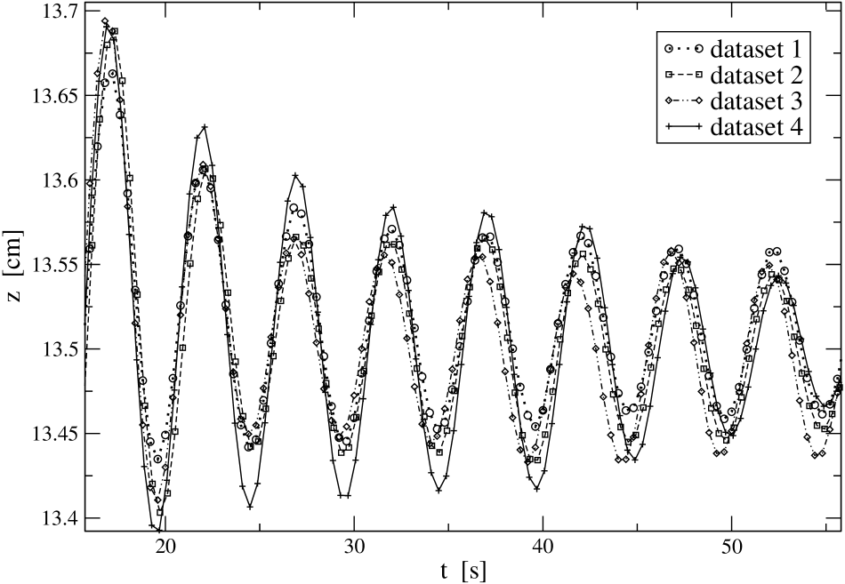
Figure 4: Height vs. time diagrams with Ball 4 in Tank 2 for 4 initial conditions as identical as possible with our experimental accuracy. The time interval shown starts with the third oscillation of the ball. The measured dots are connected with different types of lines.

5 Shadow-graphs and levitation

By illuminating the balls with a strong directed light beam, a clean shadow-graph picture of the flow pattern appears on a plane paper adjusted to the back wall of the container.

In the first part of the motion, the rapid falling of the balls, strong density inhomogeneities appear, indicating an irregular generation of lee waves (Figs 5). The characteristic wavelength is on the order of 5 cm in both the horizontal and the vertical direction. It is this strongly nonlinear set of events which can lead to the gain of a horizontal momentum of the ball, mentioned previously. The apparent random nature of the lee vortex and wave generation explains also the amplitude anomaly shown in Fig. 4. The details of the patterns in subsequent runs are very different, consequently, vertical damping and the structure of the dragged boundary layer can also be very different. These phenomena, although different in several details, can be paralleled with the chain of events occurring behind spheres in homogenous flows at similar Reynolds numbers.

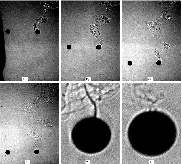
Figure 5: Shadow-graph images over the first period of motion of ball 3 in Tank 3. The time spent after release is: a) $4$ s, b) $6.4$ s, c) $10$ s, d) $16$ s, e) $22$ s, f) $54$ s. The direct image of the ball of diameter $14.6$ mm appears on the left of the shadow.

During the second part of the motion, shown on panels d)-f) of Fig. 5, when the oscillation amplitude is already small, a couple of unparallel consequences of the stratification can be identified.

First, a boundary layer around the ball consisting of light fluid dragged from the upper fluid regions in the course of the fall is clearly distinguishable. Second, the pictures also show the narrow rear jet meandering upwards from the top of the sphere. The jet ejects the light fluid ’evaporating’ from the surface of the ball back to the higher layers of the fluid. Note how the intensity of the jet diminishes with time as its light fluid supply in the boundary layer decreases. The slow ’evaporation’ of this layer explains the long term sinking of the balls (see e.g. Fig. 2a). These phenomena matches qualitatively to those found numerically in [12].

In some other cases, however, we rather found a slow asymptotic rise of the ball. One possibility for this could be the gradual swelling of the material of the ball due to its constant exposure to the liquid, such an event has been reported in [22]. In our case, the balls do not absorb water, thus their slow rising were attributed to the attachment of tiny gas bubbles to the surface of the ball. This effect is also random-like, unpredictable. It was impossible to avoid or to control it by using deaerated water since air becomes dissolved in the fluid during the process of filling up the tanks.

For a more detailed study of the rising or sinking motion, we evaluated the centres of oscillation $z_{c}$ over half periods, i.e, the mean values of subsequent displacement extrema. As Fig. 6 indicates, the oscillation centers always sink drastically over the first $5-6$ periods. This is due to the active ’evaporation’ of the light fluid from the surface, which continuously increases the effective density of the ball. Then a deepest point is reached due to an oscillation overshoot which is always followed by a slow rising, levitation, between about 50 and 200 seconds. At this stage there is still a very narrow layer of light fluid around the ball, and hence the ball might rise beyond the height defined by the condition $\varrho_{p}=\varrho_{f}$. This is followed by a sinking (Fig. 6a) if the bubble formation is weak, otherwise, a continuous rising follows (Fig. 6b).

Figure 6: Time evolution of the centres of oscillation $z_{c}$ for the motion displayed in (a) Fig. 2a and (b) Fig. 2b.

6 Oscillation frequencies

The typical frequency $\omega_{0}$ of the oscillation was determined both by measuring the average period between local maxima of the displacement and by locating the peak of the power spectrum of the function $z(t)$. Fig. 7 shows the Fourier peaks. The error estimate of the frequency is given by the halfwidth of the peak.

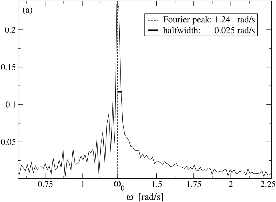
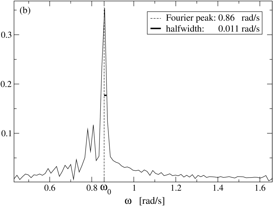
Figure 7: The power spectrum of the signals of (a) Fig. 2a and (b) Fig. 2b. The halfwidths indicating the error are marked by short horizontal intervals.

Both methods mentioned above lead to practically identical oscillation frequencies for a given measurement. The $\omega_{0}$ values fall rather close to the local BV frequency, $N$, of the height around which the long term oscillation took place. In order to see more detail, in Fig. 8 we plot the relative deviation $(\omega_{0}-N)/\omega_{0}$ from the BV frequency vs. the local BV frequency itself. There is no clear trend visible on the plot, and the average deviation is on the order of 2 percents, indicating that the added mass effect is rather weak. Note that for small added mass coefficient $\sigma$ and negligible damping coefficient (with our data $\alpha_{0}=0.042$ 1$/$s), relation (8) yields

$$\omega_{0}=\frac{N}{{(1+\sigma)}^{1/2}}\approx N(1-\sigma/2).$$ (12)

The added mass coefficient in our experiments thus can be estimated to be $\sigma\approx 0.04$. In view of the magnitude of the error, we can say that the added mass effect is practically negligible. This observation seems to be consistent with those of Ermanyuk and Gavrilov [18] who found in a linear setting that the added mass coefficient around the BV frequency tends to zero with the increasing depth of the fluid.

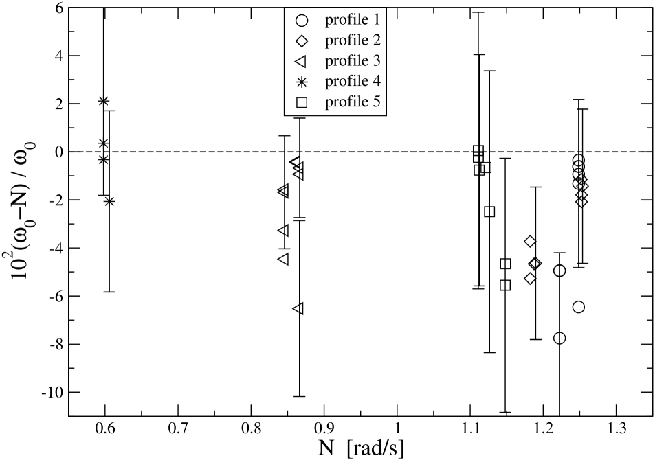
Figure 8: The relative deviation $(\omega_{0}-N)/\omega_{0}$ of the measured oscillation frequency from the local BV frequency vs the local BV frequency $N$. Different symbols mark different profiles (cf. Table 1). The average relative deviation is 2 percents, indicating an added mass coefficient $\sigma=0.04$ at most. In individual cases the $\sigma$ value turned out the be very close to zero. In order to avoid scatter, only two representative error bars per profiles are shown.

7 Amplitude dynamics

Although, as indicated earlier, the amplitudes of oscillations do not reproduce properly, these quantities can be used to obtain global information about the ball dynamics. In Fig. 9 we compare measured data with the numerical simulation of equation (5), where the added mass effect is assumed to be negligible: $\sigma=0$. In order to have a clear comparison with the exponential long term damping predicted by (6), we plot the local displacement maxima on a logarithmic scale. The initial decay appears to be similar, but after about a few tens of seconds a drastic deviation occurs: the measured data do not follow the exponential rule, they exhibit a much weaker decay. The ratio of the measured to computed amplitudes is on the order of $10^{4}$ at $t\approx 400$ s.

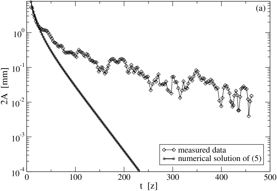
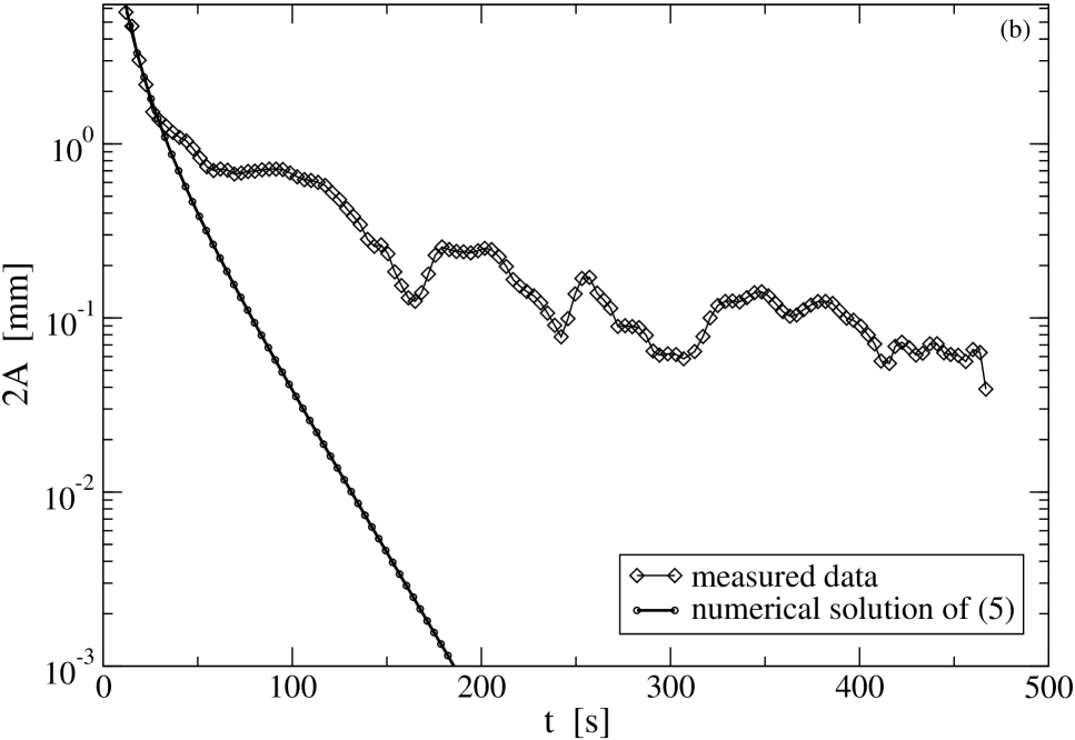
Figure 9: Local displacement maxima $2A$ measured as the difference between consequtive maxima and minima of $z$ as a function of time $t$. Dots represent measured data, while the continuous curve is the numerical solution of (5) with the first local maximum of the measured height as the initial location and zero initial velocity. Panels (a) and (b) correspond to the measurement of Fig. 2a and b, respectively.

This strong deviation is attributed to the generation of lee waves by the balls, in particular during the first period of their fall. These waves are reflected back from the boundaries and interact with the ball upon their return. Approximating the wave speed with that of linear internal waves, given by [20]

$$c=\frac{N}{(k^{2}+m^{2})^{1/2}},$$ (13)

with $k$ and $m$ as the horizontal and the vertical wave numbers, respectively, we obtain with $N\approx 1$ 1$/$s and $k=m\approx 2\pi/(5$cm) a wave speed of $c\approx 6$ mm$/$s. The time needed to return from a wall at a distance of a few dm is then on the order of $100$ s. This is the time when interference patterns first appear in Fig. 2. The viscous damping time of these waves is $(\nu(k^{2}+m^{2}))^{-1}$ which is on the order of $30$ seconds, but the damping time for waves of dm wavelength goes beyond $100$ seconds. This should be contrasted with the Stokesian damping time $1/\alpha_{0}$ of (5), which is $24$ seconds. This is the time when the deviation from the numerical solution sets in in Fig. 9.

The presence of internal waves was experimentally verified in a separate qualitative control experiment, by illuminating fluorescent dye layers in the fluid.

We conclude that the fluid motion is not negligible even long times after the initiation of the ball’s motion, due to the presence of excited and reflected internal waves. The assumption $\mathbf{u}\equiv 0$, used in the derivation of (5), therefore does not hold. After some time, the agitation by internal waves overcomes viscous damping and makes the ball oscillating much stronger than in a fluid at rest. This slow oscillation also takes place with approximately the BV frequency.

A phenomenological way of taking this into account in Eq. (5) is the switching off of the viscous damping, by replacing $c_{D}$ proportionally to $c_{D}(Re)e^{(-\alpha_{0}t)}$, where $\alpha_{0}$ is the damping coefficient (7). By solving equation

$$\ddot{z}=-\sigma\frac{\varrho_{f}(z)}{\varrho_{p}}\ddot{z}-\frac{\varrho_{p}-\varrho_{f}(z)}{\varrho_{p}}g-Ae^{-\alpha_{0}t}\frac{3\varrho_{f}(z)}{8r\varrho_{p}}\mid\dot{z}\;\mid\dot{z}c_{D}(2r\mid\dot{z}\mid/\nu),$$ (14)

a reasonable agreement with the observed data is obtained, even for long times (see Fig. 10). Coefficient $A$ should be chosen to obtain the best fit with the data. We do not claim that this phenomenological equation would provide the best model for the ball’s motion. The procedure, however, illustrates that the naive equations should be modified in view of the long lasting presence of internal waves.

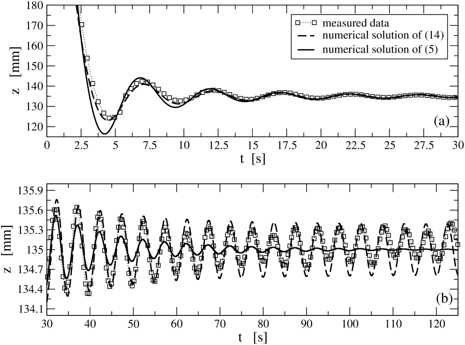
Figure 10: Comparison of a measured displacement vs. time (dataset (2) of Fig 4) with two simulations. Simulation 1 is carried out with (5), while Simulation 2 corresponds to (14) with $A=1.6$ and $\alpha_{0}=0.042\ 1/s$. In both cases $\sigma=0$. Panel (a) and (b) correspond to the early and late stage of oscillations, respectively.

To conclude this Section, we present the results of solving Larsen’s equation (11). Fig. 11 shows the $z(t)$ function obtained by starting the simulation at the first maximum upward displacement of the measured paths. In contrast to Larsen’s original observations [10], valid for very small amplitude oscillations, the numerical solution markedly deviates from the data in the course of the first oscillations already. The frequency appears to be smaller than the measured one. In addition, the long term behavior is much more damped than the numerical solution.

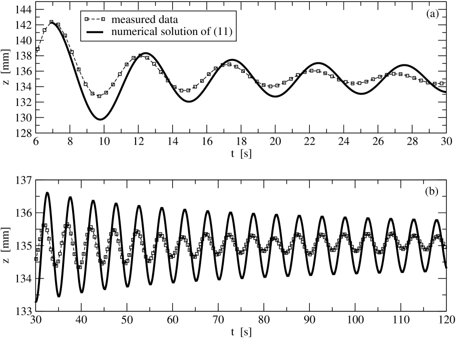
Figure 11: Comparison of measured displacement vs. time (dataset (2) of Fig 4) with Larsen’s theory (continuous line), the simulation of (11). Panel (a) and (b) correspond to the early and late stage of oscillation s, respectively.

8 Discussion and Conclusion

We stated that the history term (2) is unimportant in (1) in our experiment. One reason for this is that the relative acceleration which appears in the integrand is small in the long time dynamics, at least. Here we show that the presence of the history term does not lead to a better agreement with the measured behavior for short times either. Ignoring the doubts that (2) needs not be valid for Reynolds numbers much larger than unity, we solved Eq. (14) with the term

$$-\frac{9}{2r}\sqrt{\frac{\nu}{\pi\varrho^{2}_{p}}}\int_{0}^{t}\varrho_{f}(z(\tau))\frac{\ddot{z}}{(t-\tau)^{1/2}}\;d\tau$$ (15)

added numerically. The simulation clearly indicates (Fig. 12) a much stronger deviation from the measured data than without this term: the frequency is smaller then the measured one, and damping is much stronger.

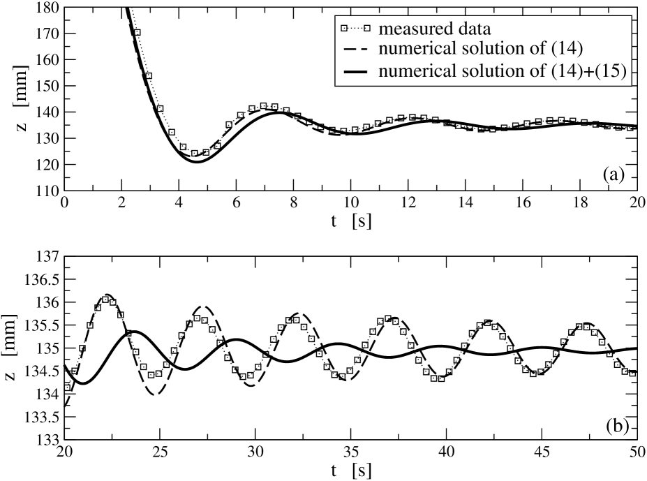
Figure 12: Comparison of the measured displacement vs. time data of Fig 2a with simulations with and without the history term. Simulation 1 is carried out with (14), and Simulation 2 is the same with term (15) added to the right hand side. In both cases $\sigma=0$, $A=1.6$ and $\alpha_{0}=0.042\ 1/s$. Panel (a) and (b) correspond to the early and late stage of oscillation s, respectively.

The fact that the history term is not appropriate for interpreting observed data does not imply of course that Equation (5) is valid. To obtain a measure of the lack of equality multiply Eq. (5) by $m_{p}$ and rearrange all terms to the left hand side to get

$$F_{r}=\underbrace{m_{p}\ddot{z}}_{(i)}+\underbrace{{\pi r^{2}}c_{D}(2r\left|{\dot{z}}\right|/\nu)\varrho_{f}\left|{\dot{z}}\right|\dot{z}/2}_{(ii)}+\underbrace{(m_{p}-m_{f}(z)){g}}_{(iii)}.$$ (16)

We applied numerical differentiation to the measured data and evaluated each term $(i)$-$(iii)$ in (16) separately, thus this formula provides us with a ‘rest force’ $F_{r}$. The result is exhibited in Fig. 13.

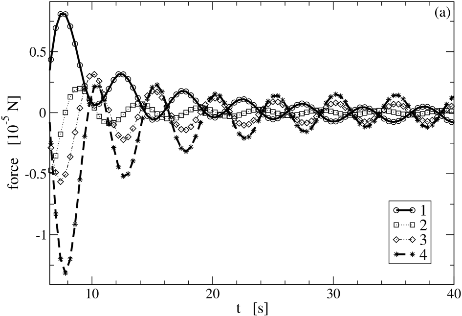
Figure 13: Contribution of the rest force and of different terms in (16) in the time series of Fig. 2a. 1: rest force $F_{r}$; 2: negative drag $(ii)$; 3: mass times acceleration $(i)$; 4: buoyancy corrected weight $(iii)$. Added mass is neglected. Panel (a) and (b) show the first $40$ s and the late stage after $250$ s, respectively.

The result clearly indicates that the rest force is never negligible. For long times the drag and the acceleration become very small, and hence the rest force is practically the negative of the buoyancy corrected weight. This further supports our view that the long time motion of the ball is very close to a passive advection in the fluid, with a very small velocity difference $\dot{\mathbf{r}}(t)-\mathbf{u}({\mathbf{r}}(t),t)$. In view of (1), it is the term $\varrho_{f}D\mathbf{u}/Dt$, i.e., the acceleration of the ambient fluid in the container, which is missing from (5).

Note that by dropping the naive assumption $\mathbf{u}\equiv 0$, the paradox of non Stokesian asymptotical behaviour mentioned in Section 4 can also be solved. If the background velocity field is nonzero, the definition (4) for the Reynolds number shall be replaced by the proper one which is based on the relative velocity rather than on $\left|{\dot{z}}\right|$. In the limit of passive advection this Reynolds number approaches 0, i.e. the ball enters Stokesian regime asymptotically.

The ambient velocity $\mathbf{u}$ appears due to the internal waves excited by the falling ball, but it also has a feedback on the ball. The problem of the velocity field and of the particle velocity cannot be decoupled, they should be treated self-consistently. In stratified fluids, therefore, there is no hope for any simple equation for ${\bf r}(t)$ which would contain the particle-free fluid velocity.

9 Acknowledgements

The authors are indebted for Detlef Lohse for a fruitful discussion. This work was supported by the Hungarian Science Foundation (OTKA) under grants TS044839 and T047233. IMJ thanks for a János Bolyai research scholarship of the Hungarian Academy of Sciences.

References

- [1] J. Boussinesq. Comptes Rendu Acad. Sci., 100:935–937, 1885.
- [2] A. B. Basset. Treatise on Hydrodynamics. Deighton Bell, London, 1888.
- [3] M. R. Maxey and J. J. Riley, Phys. Fluids 26, 883 (1983).
- [4] T. R.Auton, F. C. R. Hunt, and M. Prud’homme, J. Fluid. Mech. 197, 241 (1988).
- [5] E.E. Michaelides, J. Fluid Eng. 119, 233 (1997)
- [6] J. Magnaudet and I. Eames, Ann. Rev. Fluid Mech. 32, 659 (2000)
- [7] N. Mordant and J.F. Pinton, Eur. Phys. J. B. 38, 343 (2000)
- [8] G. Falkovich et al, Nature 453, 1045 (2005)
- [9] J. Bec et al, Phys. Fluids 17, 073301 (2005)
- [10] L. H. Larsen, Deep Sea Res. 16, 587 (1969)
- [11] J.L. Ochoa and M.L. Van Woert, unpublished report, Scripps Institution of Oceanography, pp 28 (1977)
- [12] C.R. Torres et al, J. Fluid Mech. 417, 211, (2000)
- [13] A.N. Srdić-Mitricović, N.A.Mohamed and H.J.S. Fernando, J. Fluid Mech. 381, 175 (1999)
- [14] N. Abaid et al., Phys. Fluids 16, 1567 (2004)
- [15] D.G. Hurley, J. Fluid Mech. 351, 105 (1997)
- [16] E.V. Ermanyuk, Exp. in Fluids 28, 152 (2000)
- [17] E.V. Ermanyuk and N.V. Gavrilov, J. Fluid. Mech. 451, 421 (2002)
- [18] E.V. Ermanyuk and N.V. Gavrilov, J. Fluid. Mech. 494, 33 (2003)
- [19] F.W. Roos and W.W. Willmarth, AIAA Journal 9, 285 (1971)
- [20] P.K. Kundu, Fluid Mechanics (Academic Press, San Diego, 1990)
- [21] J.M.H. Fortuin, J. Polym. Sci. 44, 505 (1960)
- [22] I.M. Jánosi, G. Szabó, and T. Tél, Eur. J. Phys. 25, 303 (2004)