Scaling of Huygens-front speedup in weakly random media

Abstract

Front propagation described by Huygens’ principle is a fundamental mechanism of spatial spreading of a property or an effect, occurring in optics, acoustics, ecology and combustion. If the local front speed varies randomly due to inhomogeneity or motion of the medium (as in turbulent premixed combustion), then the front wrinkles and its overall passage rate (turbulent burning velocity) increases. The calculation of this speedup is subtle because it involves the minimum-time propagation trajectory. Here we show mathematically that for a medium with weak isotropic random fluctuations, under mild conditions on its spatial structure, the speedup scales with the 4/3 power of the fluctuation amplitude. This result, which verifies a previous conjecture while clarifying its scope, is obtained by reducing the propagation problem to the inviscid Burgers equation with white-in-time forcing. Consequently, field-theoretic analyses of the Burgers equation have significant implications for fronts in random media, even beyond the weak-fluctuation limit.

,

1 Introduction

Phenomena from combustion [1] to seismic waves [2] to population spreading [3] can be modeled by Huygens’ principle of front propagation, first stated as a law of geometrical optics. In each application, the boundary of the affected region (idealized as a sharp front) advances normal to itself at a locally specified speed. In a uniform medium, where this speed is constant, an initially wrinkled front flattens out over time; but in a spatially varying medium, a competition occurs as wrinkling is continually reintroduced [4]. A central problem for the latter case is to determine the overall statistically steady propagation rate of the wrinkled front, which exceeds the average local speed because the front is defined by the fastest paths through the medium (first passage). Our main result, establishing under general conditions the proportionality of the speedup to the 4/3 power of the amplitude of weak fluctuations, agrees with previous heuristic analysis [4] and numerical simulations [4, 5, 6, 7], and eliminates ambiguities [8] concerning the physical relevance of the scaling. In the important case of premixed fluid combustion, the result describes the weak-advection scaling of the turbulent burning velocity [9].

Our analysis relates the front dynamics to the evolution of a pressure-free fluid obeying the white-noise-driven Burgers equation, itself a widely studied model of turbulence [10]. The results reported here enable adaptation of existing treatments of Burgers turbulence [11, 12] to estimate the prefactor of the speedup scaling and its dependence on medium structure, with implications even for the opposite, practical limit of strongly advected flames.

The propagation of a Huygens front in a general nonuniform medium is governed by the local advecting velocity of the medium as a function of time and space, $\mathbf{u}(t,\mathbf{x})$, and the local speed of propagation relative to the medium, $v(t,\mathbf{x})$. Huygens’ principle can then be stated as follows (using three-dimensional language for definiteness): If at time $t_{0}$ a point $\mathbf{x}_{0}$ lies in the affected region (including its boundary, the front), then at a slightly later time $t_{1}=t_{0}+dt$ all points in a ball of radius $v(t_{0},\mathbf{x}_{0})\,dt$ about the point $\mathbf{x}_{0}+\mathbf{u}(t_{0},\mathbf{x}_{0})\,dt$ are affected. The boundary of the affected region at $t_{1}$ (the new front) thus consists of certain points on the surfaces of balls originating from the initial front. If we consider all points on these spherical surfaces, then we automatically include those on the new front and more. Hence the front at any later time will be found among the affected points reached by arbitrary trajectories $\mathbf{x}(t)$ that start on the initial front and always move at the local speed $v$ (in any direction) relative to the medium, so that they obey

$$\left|\frac{d\mathbf{x}}{dt}-\mathbf{u}(t,\mathbf{x})\right|=v(t,\mathbf{x}).$$ (1)

Two simplifications of this general framework are physically important. First, for geometrical optics in a static or “quenched” medium with nonuniform refractive index, or for combustion of a solid propellant with nonuniform burning rate, we have $v=v(\mathbf{x})$ (time-independent fluctuations) and $\mathbf{u}\equiv\mathbf{0}$ (no advection). Note that our nonrelativistic equations do not correctly describe advection of light anyway, but are adequate for an optical medium “at rest” (where fluctuations of $v$ dominate those of $\mathbf{u}$) and for advection of sound in geometrical acoustics. Second, for idealized combustion of a premixed turbulent fluid in the limit of a very thin flame front [1], $v$ is a constant (the laminar flame speed) and $\mathbf{u}(t,\mathbf{x})$ is the turbulent flow (assumed to be unaffected by the flame). Following the derivation of our key results in Sections 2 and 3, further implications for combustion are discussed in Section 4.

2 Fronts and particles

In the general case, Eq. (1) defines a large family of “virtual” trajectories $\mathbf{x}(t)$ of which only a subset actually form the front at a given time. The criterion for the relevant trajectories is simplest if $|\mathbf{u}|<v$ everywhere, as we now assume (in Section 4 we discuss relaxing this assumption). This inequality, which is trivially satisfied for a quenched medium, ensures that advection can never sweep the front backward and thus that each point $\mathbf{y}$ is crossed by the front only once. The time of this crossing, which we call $T_{0}(\mathbf{y})$, is simply the time when the first virtual trajectory reaches $\mathbf{y}$, hence defining a first-passage problem.

To reduce the number of extraneous trajectories, we can exploit the first-passage criterion (minimization of travel time) and obtain constraints on relevant trajectories. Let us parametrize the solutions of Eq. (1) by

$$\frac{d\mathbf{x}}{dt}=\mathbf{u}+v\mathbf{n},$$ (2)

with $\mathbf{n}(t)$ a unit vector. Then (see Appendix A) a necessary condition for a first-passage trajectory is

$$\frac{d\mathbf{n}}{dt}=-P_{\mathbf{n}}(\mathsf{A}\cdot\mathbf{n}+\boldsymbol{\nabla}v),$$ (3)

where $P_{\mathbf{n}}$ denotes the projection orthogonal to $\mathbf{n}$ and $\mathsf{A}$ is the velocity gradient tensor $A_{ij}=\nabla_{i}u_{j}$; a further necessary condition is that the trajectory starts out with $\mathbf{n}$ normal to the initial front, from which it follows that $\mathbf{n}$ remains normal to the evolving front. In a quenched medium, where $\mathbf{u}$ and $\mathsf{A}$ are zero, Eqs. (2) and (3) reduce to the ray equations of geometrical optics, and there it is well known that rays propagate normal to fronts. But with advection, we see that a trajectory’s tangent vector $d\mathbf{x}/dt$ is no longer aligned with the front normal $\mathbf{n}$. As discussed in Section 4, Eqs. (2) and (3) govern front-tracking trajectories even when $|\mathbf{u}|\geq v$, but we assume $|\mathbf{u}|<v$ so that the front evolution is described by a simple first-passage problem and a single-valued function $T_{0}(\mathbf{y})$.

For first-passage purposes, then, we consider a continuum of “particles” starting simultaneously from all points on the initial front (with initial $\mathbf{n}$ given by the unit normal), and obeying Eqs. (2) and (3). If the Huygens front represents a wave phenomenon in the geometrical-optics limit of very short wavelength, then we are describing physical quasiparticles: photons for light or phonons for sound. Motivated by this physical case, we call Eqs. (2) and (3) the “law of motion” for first-passage trajectories. In premixed combustion, where the front represents a thin flame, the “particle” trajectories are mathematical constructs known as ignition curves [13].

Figure 1: Irrelevance of particles after collision. Two particles, starting from $A$ and $B$ on the initial front $i$, collide at $C$; the continuation of trajectory $AC$ (dashed) reaches $D$. If it were the first arrival, its travel time would be an absolute minimum over all virtual trajectories from $i$ to $D$, including $BCD$. Having the same minimum time, $BCD$ must also obey the law of motion, but this deterministic law does not permit the time-reversed trajectory $DC$ to split at $C$. Hence neither $ACD$ nor $BCD$ represents first passage to $D$, and the particles can be discarded upon colliding.

Even with the condition (3), not all of these particles remain on the front. The departure of particles from the front (into the interior of the affected region) is associated with “cusps” at which the normal $\mathbf{n}$ is not unique. Such cusps develop during propagation in a random medium even if the initial front is smooth [14, 15]. When two distinct particles reach the same point at the same time (necessarily with different $\mathbf{n}$), both colliding particles fall behind the front and can then be discarded, as shown in Fig. 1. (In optics and acoustics, the corresponding photons and phonons remain observable as second and later arrivals, but our scope is limited to first passage.)

The collision rule implies a correspondence between our continuum of particles and a model “fluid” without pressure or viscosity, consisting of fluid elements that move independently in response to external forces but disappear when they collide. Such a fluid is described by the inviscid Burgers equation (with suitable forcing) and the collisions are known as shocks [13, 16]. Because our particles fill a surface and not all of space, we must define the corresponding Burgers fluid more precisely. The particles, by definition, always represent the first arrival at their locations; thus if two of their paths reach the same point $\mathbf{x}$, the particles necessarily arrive at the same time $T_{0}(\mathbf{x})$ and are then discarded. Let us take the initial front to be planar and use coordinates $\mathbf{x}=(x_{\parallel},\mathbf{x}_{\perp})$ such that this plane is $x_{\parallel}=0$. Then the spatial paths of the particles can be viewed as “trajectories” $\mathbf{x}_{\perp}(x_{\parallel})$ in the “time” $x_{\parallel}$.

In this picture, a Burgers fluid exists in the lower-dimensional space $\mathbf{x}_{\perp}$, and the physical time information is carried by the function $T_{0}(x_{\parallel},\mathbf{x}_{\perp})$. Here we must introduce the assumption that the medium fluctuations are weak, i.e., that $|\mathbf{u}|$ and the changes in $v$ are both vanishingly small compared to the average value of $v$. In this limit, because trajectories cannot deviate significantly from the $x_{\parallel}$-direction without falling behind the front, the particles necessarily collide before they are deflected enough to make the function $\mathbf{x}_{\perp}(x_{\parallel})$ ill defined.

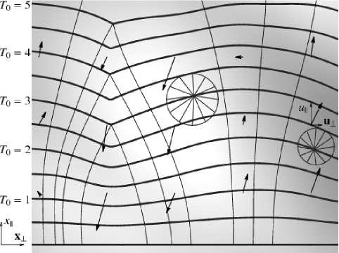
Figure 2: Complementary descriptions of first passage. A front propagates upward amid possibly time-dependent variations in $\mathbf{u}$ (arrows) and $v$ (grayscale, dark for slow). We show $\mathbf{u}$ and $v$ at the local time $T_{0}$. Snapshots of the front (thick curves) are contours of $T_{0}$; particles (thin curves) track the front until they collide at cusps. Two circles expanding from affected points illustrate Huygens’ principle. The fluctuations are weak enough to define a “fluid” using $x_{\parallel}$ as “time” for the particles. For very weak fluctuations, the front remains nearly flat, and $\mathbf{u}_{\perp}$ becomes irrelevant as it merely shifts the front without advancing it.

The law of motion for these trajectories $\mathbf{x}_{\perp}(x_{\parallel})$ could be derived from Eqs. (2) and (3), but it is simpler to obtain the Burgers equation in its conventional Eulerian form. The same minimization principle that yields Eqs. (2) and (3) also implies that $T_{0}(\mathbf{x})$ satisfies a generalized “eikonal” equation (see Appendix B)

$$\mathbf{u}\bigl{(}T_{0}(\mathbf{x}),\mathbf{x}\bigr{)}\cdot\boldsymbol{\nabla}T_{0}(\mathbf{x})+v\bigl{(}T_{0}(\mathbf{x}),\mathbf{x}\bigr{)}\,|\boldsymbol{\nabla}T_{0}(\mathbf{x})|=1.$$ (4)

The relation between $T_{0}$ and the particle trajectories is illustrated in Fig. 2 for a two-dimensional medium. Because $T_{0}$ is constant over a front, $\boldsymbol{\nabla}T_{0}$ lies along the front normal $\mathbf{n}$ (in the direction of propagation), and so the physical velocity of particles in Eq. (2) can be written

$$\frac{d\mathbf{x}}{dt}=\mathbf{u}+v\,\frac{\boldsymbol{\nabla}T_{0}}{|\boldsymbol{\nabla}T_{0}|}.$$ (5)

We next show that in the limit of weak random fluctuations, Eq. (4) reduces to the forced inviscid Burgers equation for a fluid consisting of these particles.

3 Weak-fluctuation limit

In a reference frame where the average value of $\mathbf{u}$ is zero, and in units such that the average value of $v$ is unity, let us parametrize the weak fluctuations by

$$\mathbf{u}(t,\mathbf{x}) =\epsilon\,\mathbf{U}(\epsilon t,x_{\parallel},\mathbf{x}_{\perp}),$$ (6)

$$v(t,\mathbf{x}) =1+\epsilon\,V(\epsilon t,x_{\parallel},\mathbf{x}_{\perp}),$$ (7)

where $\mathbf{U}$ and $V$ are homogeneous isotropic random fields and $\epsilon$ is taken asymptotically to zero. The time dependence of $\mathbf{u}$ and $v$ is scaled by $\epsilon$ because the natural source of time dependence is advection by $\mathbf{u}$ itself, which goes to zero with $\epsilon$. Heuristic scaling analysis [4, 6] yields the following conclusions in the $\epsilon\to 0$ limit: The medium can be considered effectively frozen ($\mathbf{U}$ and $V$ time-independent); the advection component $\mathbf{U}_{\perp}$ orthogonal to the overall propagation direction is irrelevant; the front reaches a statistically steady state over a distance of order $\epsilon^{-2/3}$; and the steady passage rate exceeds unity by an amount of order $\epsilon^{4/3}$.

Guided by these expectations, we define rescaled quantities

$$\xi =\epsilon^{p}x_{\parallel},$$ (8)

$$\tau(\xi,\mathbf{x}_{\perp}) =\epsilon^{-p}[T_{0}(x_{\parallel},\mathbf{x}_{\perp})-x_{\parallel}],$$ (9)

where we anticipate that $p=\tfrac{2}{3}$ produces a useful $\epsilon\to 0$ limit, but we also consider slightly different $p$ values to see why $\tfrac{2}{3}$ is special. The point of the rescaling is that if $\nabla_{\xi}\tau$ reaches a steady-state average value $-C$ after a finite-$\xi$ transient, then $\nabla_{\parallel}T_{0}$ averages to $1-C\epsilon^{2p}$ after a characteristic distance $x_{\parallel}\sim\epsilon^{-p}$. A planar front propagating at constant speed $v_{*}$ would have $\nabla_{\parallel}T_{0}=1/v_{*}$, and so to leading order the passage rate in the random medium is

$$v_{*}=1+C\epsilon^{2p}.$$ (10)

Our main result is a demonstration that for $p=\tfrac{2}{3}$, the rescaled front is governed by a forced Burgers equation that reaches such a steady state, thus implying $\epsilon^{4/3}$ dependence of the speedup.

Substituting Eqs. (6)–(9) into the eikonal equation (4), we find

$$\begin{split}&\epsilon\,U_{\parallel}(\epsilon^{1-p}\xi+\epsilon^{1+p}\tau,\epsilon^{-p}\xi,\mathbf{x}_{\perp})\,(1+\epsilon^{2p}\nabla_{\xi}\tau)\\ &\qquad+\epsilon\,\mathbf{U}_{\perp}(\epsilon^{1-p}\xi+\epsilon^{1+p}\tau,\epsilon^{-p}\xi,\mathbf{x}_{\perp})\cdot\epsilon^{p}\boldsymbol{\nabla}_{\perp}\tau\\ &\qquad+[1+\epsilon\,V(\epsilon^{1-p}\xi+\epsilon^{1+p}\tau,\epsilon^{-p}\xi,\mathbf{x}_{\perp})]\\ &\qquad\qquad\times\sqrt{(1+\epsilon^{2p}\nabla_{\xi}\tau)^{2}+\epsilon^{2p}|\boldsymbol{\nabla}_{\perp}\tau|^{2}}=1.\end{split}$$ (11)

For $\tfrac{1}{2}<p<1$, this result (multiplied by $\epsilon^{-2p}$) simplifies considerably as $\epsilon\to 0$:

$$\begin{split}\nabla_{\xi}\tau+\tfrac{1}{2}|\boldsymbol{\nabla}_{\perp}\tau|^{2}={}&{-}\epsilon^{1-2p}\,U_{\parallel}(0,\epsilon^{-p}\xi,\mathbf{x}_{\perp})\\ &-\epsilon^{1-2p}\,V(0,\epsilon^{-p}\xi,\mathbf{x}_{\perp})\\ \equiv{}&\eta(\xi,\mathbf{x}_{\perp}).\end{split}$$ (12)

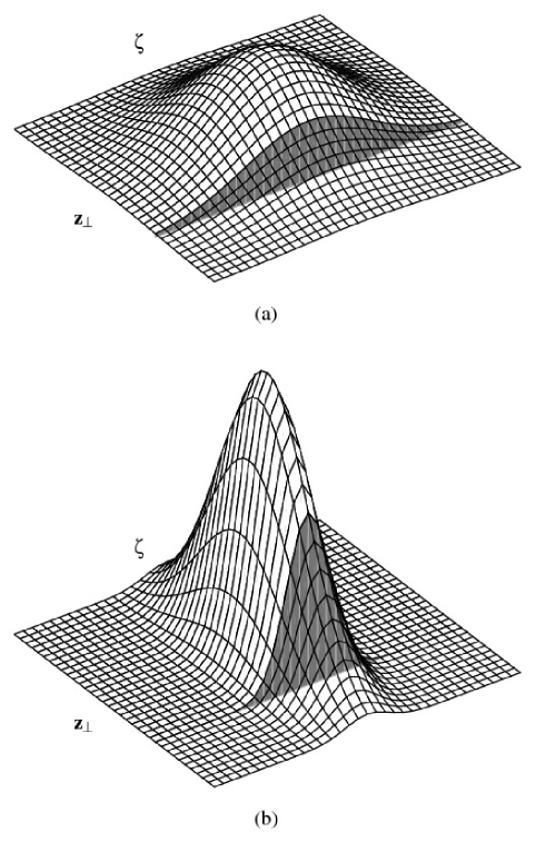
Figure 3: Convergence of weak fluctuations to white noise. Choosing a simple random medium with $\langle\gamma(\mathbf{0})\,\gamma(\mathbf{z})\rangle\sim\exp(-z^{2})$, we show the two-point correlation function of $\eta$, Eq. (13), for $\epsilon=1$ (a) and $\epsilon=0.2$ (b). As $\epsilon\to 0$, the function is infinitely compressed in the “time” direction $\zeta$, but with the choice of scaling exponent $p=\tfrac{2}{3}$, its time integral at a given $\mathbf{z}_{\perp}$ (shaded area) remains fixed. This integral gives the $\mathbf{z}_{\perp}$-dependent coefficient of a delta function that describes spatially correlated white-in-time noise.

As expected, both the component $\mathbf{U}_{\perp}$ and the time dependence of the medium go away in this limit. The front responds to the frozen random field $\gamma(x_{\parallel},\mathbf{x}_{\perp})\equiv-(U_{\parallel}+V)$, which is homogeneous but not generally isotropic because a specific component of $\mathbf{U}$ is selected. The rescaled function $\eta(\xi,\mathbf{x}_{\perp})=\epsilon^{1-2p}\,\gamma(\epsilon^{-p}\xi,\mathbf{x}_{\perp})$ appears to diverge as $\epsilon\to 0$, but its dependence on the “time” $\xi$ also becomes more and more rapid, and in fact with $p=\tfrac{2}{3}$ it converges under mild assumptions to a white-noise process in $\xi$. The two-point correlation function of $\eta$ is

$$\begin{split}\langle\eta(\xi,\mathbf{x}_{\perp})\,\eta(\xi&+\zeta,\mathbf{x}_{\perp}+\mathbf{z}_{\perp})\rangle=\langle\eta(0,\mathbf{0})\,\eta(\zeta,\mathbf{z}_{\perp})\rangle\\ ={}&\epsilon^{2-3p}\epsilon^{-p}\langle\gamma(0,\mathbf{0})\,\gamma(\epsilon^{-p}\zeta,\mathbf{z}_{\perp})\rangle\\ \xrightarrow{\epsilon\to 0}{}&\epsilon^{2-3p}\,\delta(\zeta)\int_{-\infty}^{\infty}da\,\langle\gamma(0,\mathbf{0})\,\gamma(a,\mathbf{z}_{\perp})\rangle,\end{split}$$ (13)

where the rescaled expression is squeezed into a Dirac delta function in $\xi$, corresponding to white noise, times a factor that remains finite for $p=\tfrac{2}{3}$. Because any interval of $\xi$ corresponds to an infinitely long sample of the medium, $\eta$ is a Gaussian random field even if $\gamma$ is not, provided the correlations of $\gamma$ decay fast enough with $x_{\parallel}$ so that the central limit theorem is applicable. (For example, in homogeneous turbulence with strong intermittency, the statistics of $\gamma$ are highly non-Gaussian; but because the flow decorrelates over a few integral scales, the long-term effect on the front is given as $\epsilon\to 0$ by Gaussian white noise.) Despite becoming white in “time”, the $\eta$ correlation function (13) remains smooth in “space”; this $\epsilon\to 0$ limit is visualized in Fig. 3.

To confirm that Eq. (12) with $p=\tfrac{2}{3}$ describes a Burgers fluid, note that

$$\boldsymbol{\nabla}T_{0}=(1+\epsilon^{4/3}\nabla_{\xi}\tau,\epsilon^{2/3}\boldsymbol{\nabla}_{\perp}\tau),$$ (14)

and so the physical particle velocity (5) gives

$$\begin{split}\mathbf{w}\equiv{}&\frac{d\mathbf{x}_{\perp}}{d\xi}=\epsilon^{-2/3}\,\frac{d\mathbf{x}_{\perp}/dt}{dx_{\parallel}/dt}\\ ={}&\epsilon^{-2/3}\frac{\epsilon\mathbf{U}_{\perp}+(1+\epsilon V)\epsilon^{2/3}\boldsymbol{\nabla}_{\perp}\tau/|\boldsymbol{\nabla}T_{0}|}{\epsilon U_{\parallel}+(1+\epsilon V)(1+\epsilon^{4/3}\nabla_{\xi}\tau)/|\boldsymbol{\nabla}T_{0}|}\\ \xrightarrow{\epsilon\to 0}{}&\boldsymbol{\nabla}_{\perp}\tau\end{split}$$ (15)

for the Burgers “velocity” $\mathbf{w}$ in the time variable $\xi$. The $\mathbf{x}_{\perp}$ gradient of Eq. (12) then yields

$$\nabla_{\xi}\mathbf{w}+(\mathbf{w}\cdot\boldsymbol{\nabla}_{\perp})\mathbf{w}=\boldsymbol{\nabla}_{\perp}\eta(\xi,\mathbf{x}_{\perp}),$$ (16)

which is the inviscid Burgers equation with white-noise forcing [17]. Since the fluid elements are precisely the front-tracking particles, cusp singularities in the front are described by the standard jump conditions for Burgers shocks [18].

Because $\eta$ averages to zero, Eq. (12) implies that in a steady state

$$C\equiv-\langle\nabla_{\xi}\tau\rangle=\tfrac{1}{2}\langle|\boldsymbol{\nabla}_{\perp}\tau|^{2}\rangle=\tfrac{1}{2}\langle w^{2}\rangle.$$ (17)

Thus the prefactor of $\epsilon^{4/3}$ in the front speedup is the steady-state energy density of the white-noise-driven Burgers fluid. It was shown rigorously [17] that for white noise that is periodic in space with any given smooth correlation function, there exists a unique statistically steady state for the inviscid Burgers equation. This holds in any spatial dimension, generalizing a previous result [19] for the one-dimensional Burgers equation (corresponding to two-dimensional propagation). Since an assumption of spatial periodicity is an accepted device for treating bulk properties, we have convincing evidence that $C$ is well defined for a realistic smooth random medium given its two-point spatial correlation function $f(\mathbf{z})\equiv\langle\gamma(\mathbf{0})\,\gamma(\mathbf{z})\rangle$, which determines the $\eta$ correlation function (13), independent of higher statistics.

For geometrical optics in a quenched random medium, the essential rescaling technique and a reduction to white noise were previously demonstrated at the level of the ray equations [14, 20], but the first-passage problem and the disappearance of rays at cusps (leading to the inviscid Burgers equation) were not considered. On the other hand, the analogous shock singularities of the Burgers fluid can be eliminated by a variant of Eq. (16) with an additional term $-\nu\nabla_{\perp}^{2}\mathbf{w}$ on the left, known as the viscous Burgers equation [11]. (The viscosity $\nu>0$ smooths the shocks.) The corresponding variant of Eq. (12), with $-\nu\nabla_{\perp}^{2}\tau$ on the left, is a form of the Kardar-Parisi-Zhang (KPZ) equation for interface growth [21]. Under forcing that is continuous in space and time, the solution of these equations is known to approach as $\nu\to 0$ a limiting “viscosity solution” that reproduces the inviscid shocks [22]. Under white-noise forcing, the steady state of the viscous Burgers equation was analyzed using field theory [10, 11], but the $\nu\to 0$ limit is more subtle. Fortunately, a recent theorem [23] establishes that the viscous white-noise steady state converges to the inviscid one, making the $\nu\to 0$ results of field theory applicable to the $\epsilon\to 0$ limit of Huygens propagation. A previous description of weakly advected flames based on the KPZ equation [9] assumed a white-noise velocity field for convenience, but did not observe that it could arise from a realistic smooth medium by rescaling, yielding the $\epsilon^{4/3}$ law in the process.

4 Conclusion

The newly established equivalence between $\nu\to 0$ Burgers turbulence and the $\epsilon\to 0$ propagation problem allows adaptation of field-theoretic [11] and numerical [12] methods previously applied to the former in order to analyze the latter. Results of this adaptation will be reported elsewhere. The results obtained here already indicate the central importance of the spatial structure of the random medium to front propagation. Indeed, a sufficiently anisotropic medium can have a different scaling law, explaining the $\epsilon^{2}$ dependence of the speedup derived for one such medium [8]. There, a flow $\mathbf{U}$ is constructed by adding (with random phases) a finite number of Fourier modes, none of whose wavevectors are exactly orthogonal to $x_{\parallel}$. In this homogeneous but anisotropic medium, the integral in Eq. (13) oscillates and averages to zero. The amplitude of the white noise then vanishes and so $C=0$, indicating correctly that the speedup goes to zero faster than $\epsilon^{4/3}$. As we will subsequently report, $\epsilon^{2}$ scaling in this random medium is a direct result of the gross anisotropy—similar to the original argument for $\epsilon^{2}$ scaling [24], which was validated for an $x_{\parallel}$-periodic medium [25]. We have here established $\epsilon^{4/3}$ scaling as the generic case, applying to random media with a finite spectral density orthogonal to $x_{\parallel}$, such as isotropic media. (Although isotropic flows $\mathbf{U}$ lead to anisotropic $\gamma$, the generic scaling still holds because in realistic cases the relevant transverse modes of $U_{\parallel}$ have a finite spectral density; in particular, they are not constrained even if incompressibility is assumed. Furthermore, generic quantitative deviations from flow isotropy that maintain this finiteness do not alter the scaling.)

There is a different sense in which $\epsilon^{2}$ scaling exists even for isotropic media: as a transient starting from a flat initial front. Before cusps form, a linearized approximation is adequate; we expect front tilts proportional to $\epsilon$ and thus a speedup proportional to $\epsilon^{2}$, both systematically increasing with time. In the Burgers picture, there is an order-unity interval of $\xi$ before shocks become important, during which the steady energy input results in an energy density proportional to $\xi$. The transient speedup is therefore proportional to $\epsilon^{4/3}\xi=\epsilon^{2}x_{\parallel}$. As stated previously, our analysis applies after a distance $x_{\parallel}\sim\epsilon^{-2/3}$, where a steady-state $\epsilon^{4/3}$ speedup is attained.

For premixed combustion applications, while weak advection is a useful limiting case, the strong-advection limit $|\mathbf{u}|\gg v$ is more important [1]. Because the white-noise reduction and effective freezing of the medium no longer apply, we expect the strongly turbulent burning velocity to depend not only on the two-point spatial correlation function $f$ but also on more complicated spatiotemporal flow statistics. A widely used isotropic-turbulence burning-velocity model [26] fails to incorporate this nonuniversality and also reduces to $\epsilon^{2}$ instead of $\epsilon^{4/3}$ scaling in the weak limit.

A further implication of our analysis for strong turbulence comes from a monotonicity property: For a given initial front and flow $\mathbf{u}(t,\mathbf{x})$, all fluid elements burned by a later time for laminar flame speed $v_{1}$ are also burned for $v_{2}>v_{1}$. Thus the turbulent burning velocity can only increase with $v$, even into the weak-advection regime $v\gg|\mathbf{u}|$. The aforementioned field-theoretic constraints on the weakly turbulent burning velocity then establish useful boundedness properties of the strongly turbulent one. Finally, although we derived the trajectory equations (2) and (3) assuming $|\mathbf{u}|<v$, they are Galilean invariant and are thus valid in general, because Huygens’ principle is local and we can switch to a reference frame where $|\mathbf{u}|<v$ in a neighborhood of a given event. The trajectory equations do not require a continuous representation of the front for constructing the normal $\mathbf{n}$ (except initially) and therefore may be useful in numerical studies at all turbulence intensities, although for very low intensity it is advantageous to exploit the Burgers equivalence.

Appendix A Law of motion for first-passage trajectories

The first arrival at an arbitrary point from an initial front is a constrained optimum: the result of minimizing the travel time $T$ among virtual trajectories $\mathbf{x}(t)$ obeying Eq. (1), or equivalently (2) with arbitrary unit $\mathbf{n}(t)$, such that $\mathbf{a}\equiv\mathbf{x}(0)$ is on the initial front and $\mathbf{y}\equiv\mathbf{x}(T)$ is the desired endpoint. Using the method of Lagrange multipliers, we eliminate some of the constraints by introducing auxiliary variables. Consider a trajectory $\mathbf{x}(t)$ obeying the constraints. If the travel-time variation $\delta T$ vanishes for all infinitesimal trajectory variations $\delta\mathbf{x}(t)$ that preserve the constraints (a necessary condition for a minimum), then for trajectory variations that keep $\mathbf{a}$ on the initial front but are otherwise arbitrary, $\delta T$ must be proportional to the deviations from the other constraints:

$$\delta T=\delta\mathbf{y}\cdot\boldsymbol{\kappa}+\int_{0}^{T}dt\,\delta[\mathbf{u}(t,\mathbf{x})+v(t,\mathbf{x})\,\mathbf{n}(t)-\dot{\mathbf{x}}(t)]\cdot\boldsymbol{\lambda}(t).$$ (18)

Here the overdot denotes a time derivative, $\boldsymbol{\kappa}$ is the Lagrange multiplier for the constraint on the endpoint $\mathbf{y}$ and $\boldsymbol{\lambda}(t)$ is the Lagrange multiplier for the time-dependent constraint (2). Equation (18) must hold for all infinitesimal variations $\delta T$, $\delta\mathbf{x}(t)$, $\delta\mathbf{n}(t)$ as long as the starting point $\mathbf{a}$ remains on the initial front and $\mathbf{n}(t)$ remains a unit vector.

The total variation of $\mathbf{y}=\mathbf{x}(T)$ is $\delta\mathbf{y}=\delta\mathbf{x}(T)+\dot{\mathbf{x}}(T)\,\delta T$ (i.e., the endpoint can be changed either by altering the trajectory itself or by following it for a longer or shorter time). Accordingly, Eq. (18) becomes

$$\delta T={} [\delta\mathbf{x}(T)+\dot{\mathbf{x}}(T)\,\delta T]\cdot\boldsymbol{\kappa}$$

$$+\int_{0}^{T}dt\,[ \delta\mathbf{x}(t)\cdot\mathsf{A}(t,\mathbf{x})+\delta\mathbf{x}(t)\cdot\boldsymbol{\nabla}v(t,\mathbf{x})\,\mathbf{n}(t)$$

$$+v(t,\mathbf{x})\,\delta\mathbf{n}(t)-\delta\dot{\mathbf{x}}(t)]\cdot\boldsymbol{\lambda}(t).$$ (19)

Because $\delta\mathbf{n}$ is constrained only by $\delta\mathbf{n}\cdot\mathbf{n}=0$, the term proportional to $\delta\mathbf{n}\cdot\boldsymbol{\lambda}$ shows that $\boldsymbol{\lambda}$ must be along $\mathbf{n}$, say $\boldsymbol{\lambda}(t)=\mathbf{n}(t)\,\mu(t)$. Next we integrate $-\delta\dot{\mathbf{x}}\cdot\boldsymbol{\lambda}$ by parts to obtain

$$\delta T={} \dot{\mathbf{x}}(T)\cdot\boldsymbol{\kappa}\,\delta T+\delta\mathbf{x}(T)\cdot[\boldsymbol{\kappa}-\mathbf{n}(T)\,\mu(T)]$$

$$+\delta\mathbf{a}\cdot\mathbf{n}(0)\,\mu(0)$$

$$+\int_{0}^{T}dt\,\delta\mathbf{x}(t)\cdot[ \mathsf{A}(t,\mathbf{x})\cdot\mathbf{n}(t)\,\mu(t)+\boldsymbol{\nabla}v(t,\mathbf{x})\,\mu(t)$$

$$+\dot{\mathbf{n}}(t)\,\mu(t)+\mathbf{n}(t)\,\dot{\mu}(t)].$$ (20)

Validity of Eq. (20) for arbitrary $\delta T$ gives

$$1=\dot{\mathbf{x}}(T)\cdot\boldsymbol{\kappa}=[\mathbf{u}(T,\mathbf{y})+v(T,\mathbf{y})\,\mathbf{n}(T)]\cdot\boldsymbol{\kappa}.$$ (21)

Validity for arbitrary $\delta\mathbf{x}(T)$ gives

$$\boldsymbol{\kappa}=\mathbf{n}(T)\,\mu(T).$$ (22)

Validity for arbitrary $\delta\mathbf{a}$ tangent to the initial front shows that $\mathbf{n}(0)$ is in the normal direction, as claimed. Because any instant of time can be considered “initial”, a first-passage trajectory always has $\mathbf{n}$ normal to the evolving front (while the trajectory remains on the front). Finally, validity for arbitrary $\delta\mathbf{x}(t)$ gives (upon projecting orthogonal to $\mathbf{n}$)

$$\dot{\mathbf{n}}(t)=-P_{\mathbf{n}(t)}\bigl{(}\mathsf{A}(t,\mathbf{x})\cdot\mathbf{n}(t)+\boldsymbol{\nabla}v(t,\mathbf{x})\bigr{)},$$ (23)

which justifies Eq. (3) and, together with Eq. (2), defines the law of motion. Results equivalent to Eqs. (2) and (3) were obtained in geometrical acoustics by assuming, rather than proving, that $\mathbf{n}$ is the front normal [27].

Our variational method is reminiscent of the reciprocal Hamilton principle [28], a modern contribution to the classical mechanics of particles. Whereas the ordinary Hamilton least-action principle requires the action to be stationary under variation of a trajectory between two points over a fixed time interval, the reciprocal Hamilton principle requires the travel time to be stationary under variation of a trajectory with fixed action. Both principles are equivalent to Newton’s or Hamilton’s equations of motion. In our problem, Eqs. (2) and (3) can in fact be derived from a Hamiltonian

$$H(t,\mathbf{x},\boldsymbol{\lambda})=\mathbf{u}(t,\mathbf{x})\cdot\boldsymbol{\lambda}+v(t,\mathbf{x})\,|\boldsymbol{\lambda}|,$$ (24)

if we treat $\boldsymbol{\lambda}$ (previously a Lagrange multiplier) as the canonical momentum and define $\mathbf{n}\equiv\boldsymbol{\lambda}/|\boldsymbol{\lambda}|$. The corresponding action is

$$\begin{split}S&\equiv\int_{0}^{T}dt\,[\boldsymbol{\lambda}(t)\cdot\dot{\mathbf{x}}(t)-H(t,\mathbf{x},\boldsymbol{\lambda})]\\ &=\int_{0}^{T}dt\,[\dot{\mathbf{x}}(t)-\mathbf{u}(t,\mathbf{x})-v(t,\mathbf{x})\,\mathbf{n}(t)]\cdot\boldsymbol{\lambda}(t),\end{split}$$ (25)

which vanishes for “Huygens” trajectories that obey Eq. (2), as well as for many other trajectories that do not.

The reciprocal Hamilton principle implies that a first-passage trajectory has stationary travel time not only among Huygens trajectories but also among the wider class with $S=0$. One might suppose we could consider the trajectory with absolute minimum (hence stationary) travel time in the $S=0$ class, apply the reciprocal Hamilton principle to obtain the equations of motion (2) and (3) and then observe that such a trajectory obeys the fundamental constraint (1) of Huygens propagation and thus represents the physical first passage. But this shortcut fails because of an important technicality: Among trajectories with $S=0$, there is no absolute minimum travel time between two points. For simplicity, take a quenched medium with $\mathbf{u}\equiv\mathbf{0}$. A sufficient condition for $S=0$ is that $\dot{\mathbf{x}}\cdot\boldsymbol{\lambda}=v|\boldsymbol{\lambda}|$, i.e., the component of $\dot{\mathbf{x}}$ along $\boldsymbol{\lambda}$ equals $v$. A suitable $\boldsymbol{\lambda}$ exists as long as $|\dot{\mathbf{x}}|\geq v$, and so the $S=0$ class includes arbitrarily fast trajectories. Therefore the reciprocal Hamilton principle is not a sound basis for deriving the first-passage law of motion, although that law can be expressed in Hamiltonian form. Instead, we have derived the law of motion from the correctly constrained variational principle.

Appendix B Generalized eikonal equation

The extra implications of our variational principle give a useful result for the spatial dependence of the first-passage time $T_{0}(\mathbf{y})$. Equation (18) shows that for variations restricted to first-passage trajectories ($T=T_{0}$), so that the variation inside the integral is zero, we have $\delta T_{0}=\boldsymbol{\kappa}\cdot\delta\mathbf{y}$ and thus $\boldsymbol{\nabla}T_{0}=\boldsymbol{\kappa}$. Equation (22) and $|\mathbf{n}|=1$ then give

$$\mathbf{n}=\frac{\boldsymbol{\nabla}T_{0}}{|\boldsymbol{\nabla}T_{0}|},$$ (26)

confirming that $\mathbf{n}$ is always normal to the front. Substituting into Eq. (21), we find

$$\mathbf{u}(T_{0},\mathbf{y})\cdot\boldsymbol{\nabla}T_{0}+v(T_{0},\mathbf{y})\,|\boldsymbol{\nabla}T_{0}|=1.$$ (27)

A form of this equation is known in geometrical acoustics [29] as a generalization of the “eikonal” equation of geometrical optics. We see that it follows directly from Huygens’ principle in a time-dependent advected medium.

In fact, a closely related “$G$ equation” was obtained for idealized premixed combustion [15, 30]:

$$\dot{G}+\mathbf{u}\cdot\boldsymbol{\nabla}G=v|\boldsymbol{\nabla}G|,$$ (28)

where a particular “level surface” of the function $G$, say the set of points $\mathbf{y}$ where $G(t,\mathbf{y})=0$, represents the front at time $t$. The gradient of the identity $G\bigl{(}T_{0}(\mathbf{y}),\mathbf{y}\bigr{)}=0$ gives $\boldsymbol{\nabla}T_{0}=-\boldsymbol{\nabla}G/\dot{G}$ and proves the equivalence with Eq. (27). The $G$ equation corresponds to the Hamilton-Jacobi equation of classical mechanics [31], with Hamiltonian (24), momentum $\boldsymbol{\lambda}=-\boldsymbol{\nabla}G$ and Hamilton’s principal function $-G$. Although the equations of motion for this Hamiltonian reproduce (2) and (3), in general such trajectories (“characteristics” of the Hamilton-Jacobi equation) do not move with level surfaces of Hamilton’s principal function. They do so for this Hamiltonian because the action (25) vanishes, reflecting the equality of group and phase velocity (absence of dispersion) in Huygens propagation.

References

- [1] F. A. Williams, Combustion Theory, 2nd Edition, Benjamin/Cummings, Menlo Park, California, 1985.
- [2] J. A. Sethian, A. M. Popovici, 3-D traveltime computation using the fast marching method, Geophysics 64 (1999) 516–523.
- [3] J. D. Murray, Mathematical Biology, 3rd Edition, Springer, New York, 2002.
- [4] A. R. Kerstein, W. T. Ashurst, Propagation rate of growing interfaces in stirred fluids, Phys. Rev. Lett. 68 (1992) 934–937.
- [5] M. Roth, G. Müller, R. Snieder, Velocity shift in random media, Geophys. J. Int. 115 (1993) 552–563.
- [6] A. R. Kerstein, W. T. Ashurst, Passage rates of propagating interfaces in randomly advected media and heterogeneous media, Phys. Rev. E 50 (1994) 1100–1113.
- [7] A. C. Martí, F. Sagués, J. M. Sancho, Front dynamics in turbulent media, Phys. Fluids 9 (1997) 3851–3857.
- [8] V. Akkerman, V. Bychkov, Turbulent flame and the Darrieus–Landau instability in a three-dimensional flow, Combust. Theory Modelling 7 (2003) 767–794.
- [9] S. P. Fedotov, The problem of flame propagation in a random velocity field: Weak turbulence limit, J. Phys. A 28 (1995) 2057–2064.
- [10] A. M. Polyakov, Turbulence without pressure, Phys. Rev. E 52 (1995) 6183–6188.
- [11] J. P. Bouchaud, M. Mézard, G. Parisi, Scaling and intermittency in Burgers turbulence, Phys. Rev. E 52 (1995) 3656–3674.
- [12] T. Gotoh, R. H. Kraichnan, Steady-state Burgers turbulence with large-scale forcing, Phys. Fluids 10 (1998) 2859–2866.
- [13] J. A. Sethian, Curvature and the evolution of fronts, Commun. Math. Phys. 101 (1985) 487–499.
- [14] B. S. White, The stochastic caustic, SIAM J. Appl. Math. 44 (1984) 127–149.
- [15] A. R. Kerstein, W. T. Ashurst, F. A. Williams, Field equation for interface propagation in an unsteady homogeneous flow field, Phys. Rev. A 37 (1988) 2728–2731.
- [16] P. Bernard, The asymptotic behaviour of solutions of the forced Burgers equation on the circle, Nonlinearity 18 (2005) 101–124.
- [17] R. Iturriaga, K. Khanin, Burgers turbulence and random Lagrangian systems, Commun. Math. Phys. 232 (2003) 377–428.
- [18] P. D. Lax, Hyperbolic Systems of Conservation Laws and the Mathematical Theory of Shock Waves, SIAM, Philadelphia, 1973.
- [19] W. E, K. Khanin, A. Mazel, Y. Sinai, Invariant measures for Burgers equation with stochastic forcing, Ann. Math. 151 (2000) 877–960.
- [20] B. Nair, B. S. White, High-frequency wave propagation in random media: A unified approach, SIAM J. Appl. Math. 51 (1991) 374–411.
- [21] M. Kardar, G. Parisi, Y.-C. Zhang, Dynamic scaling of growing interfaces, Phys. Rev. Lett. 56 (1986) 889–892.
- [22] M. G. Crandall, P.-L. Lions, Viscosity solutions of Hamilton-Jacobi equations, Trans. Am. Math. Soc. 277 (1983) 1–42.
- [23] D. Gomes, R. Iturriaga, K. Khanin, P. Padilla, Viscosity limit of stationary distributions for the random forced Burgers equation, Moscow Math. J. 5 (2005) 613–632.
- [24] P. Clavin, F. A. Williams, Theory of premixed-flame propagation in large-scale turbulence, J. Fluid Mech. 90 (1979) 589–604.
- [25] W. T. Ashurst, G. I. Sivashinsky, On flame propagation through periodic-flow fields, Combust. Sci. Tech. 80 (1991) 159–164.
- [26] V. Yakhot, Propagation velocity of premixed turbulent flames, Combust. Sci. Tech. 60 (1988) 191–214.
- [27] R. Engelke, Ray trace acoustics in unsteady inhomogeneous flow, J. Acoust. Soc. Am. 56 (1974) 1291–1292.
- [28] C. G. Gray, G. Karl, V. A. Novikov, The four variational principles of mechanics, Ann. Phys. (NY) 251 (1996) 1–25.
- [29] A. D. Pierce, Acoustics: An Introduction to Its Physical Principles and Applications, Acoustical Society of America, Woodbury, New York, 1989.
- [30] F. A. Williams, Turbulent combustion, in: J. D. Buckmaster (Ed.), The Mathematics of Combustion, SIAM, Philadelphia, 1985, pp. 97–131.
- [31] H. Goldstein, C. P. Poole, J. L. Safko, Classical Mechanics, 3rd Edition, Addison-Wesley, Reading, Massachusetts, 2002.