A study of H+H₂ and several H-bonded molecules by phaseless auxiliary-field quantum Monte Carlo with planewave and Gaussian basis sets

Abstract

We present phaseless auxiliary-field (AF) quantum Monte Carlo (QMC) calculations of the ground states of some hydrogen-bonded systems. These systems were selected to test and benchmark different aspects of the new phaseless AF QMC method. They include the transition state of H+H₂ near the equilibrium geometry and in the van der Walls limit, as well as H₂O, OH, and H₂O₂ molecules. Most of these systems present significant challenges for traditional independent-particle electronic structure approaches, and many also have exact results available. The phaseless AF QMC method is used either with a planewave basis with pseudopotentials or with all-electron Gaussian basis sets. For some systems, calculations are done with both to compare and characterize the performance of AF QMC under different basis sets and different Hubbard-Stratonovich decompositions. Excellent results are obtained using as input single Slater determinant wave functions taken from independent-particle calculations. Comparisons of the Gaussian based AF QMC results with exact full configuration show that the errors from controlling the phase problem with the phaseless approximation are small. At the large basis-size limit, the AF QMC results using both types of basis sets are in good agreement with each other and with experimental values.

I Introduction

Quantum Monte Carlo (QMC) methods QMC_rmp ; zhang_krakauer offer a unique way to treat explicitly the many-electron problem. The many-body solution is obtained in a statistical sense by building stochastic ensembles that sample the wave function in some representation. This leads to computational costs that scale as a low power with the number of particles and basis size. Although in practice QMC methods are often not exact, they have shown considerably greater accuracy than traditional electronic structure approaches in a variety of systems. They are increasingly applied and are establishing themselves as a unique approach for studying both realistic materials and important model systems.

Recently, a new phaseless auxiliary-field QMC (AF QMC) method has been developed and applied for electronic structure calculations zhang_krakauer ; gafqmc . This method is formulated in a many-particle Hilbert space whose span is defined by a single-particle basis set. The freedom to choose the basis set can potentially result in increased efficiency. This can be very useful both for quantum chemistry applications and in calculations with model Hamiltonians. Further, it is straightforward in this method to exploit well-established techniques of independent-particle theories for the chosen basis set. The ability to use any single-particle basis is thus an attractive feature of the AF QMC method. On the other hand, the use of finite basis sets requires monitoring the convergence of calculated properties and extrapolation of the results to the infinite basis size limit.

Planewave and Gaussian basis sets are the most widely used in electronic structure calculations. Planewaves are appealing, because they form a complete orthonormal basis set, and convergence with respect to basis size is easily controlled. A single energy cutoff parameter $E_{{\rm cut}}$ controls the basis size by including all planewaves with wavevector ${\bf{k}}$ such that ${\bf{k}}^{2}/2<E_{\rm{cut}}$ (Hartree atomic units are used throughout the paper). The infinite basis limit is approached by simply increasing $E_{{\rm cut}}$ payne_rmp . Localized basis sets, by contrast, offer a compact and efficient representation of the system’s wavefunctions. Moreover, the resulting sparsity of the Hamiltonians can be very useful in $\cal{O}(N)$ methods. Achieving basis set convergence, however, requires more care. For Gaussian basis sets, quantum chemists have compiled lists of basis sets of increasing quality for most of the elements basis_sets_web . Some of these basis sets have been designed for basis extrapolation not only in mean-field theories, but also in correlated calculations dunning1 ; dunning2 .

The AF QMC method also provides a different route to controlling the Fermion sign problem FermionSign ; FermionSign2 ; Zhang ; zhang_krakauer . The standard diffusion Monte Carlo (DMC) method QMC_rmp ; anderson_fixednode ; dmc employs the fixed-node approximation anderson_fixednode in real coordinate space. The AF QMC method uses random walks in a manifold of Slater determinants (in which antisymmetry is automatically imposed on each random walker). The Fermion sign/phase problem is controlled approximately according to the overlap of each random walker (Slater determinant) with a trial wave function. Applications of the phaseless AF QMC method to date, including second-row systems zhang_krakauer and transition metal molecules alsaidi_tio_mno with planewave basis sets, and first-row gafqmc and post-d gafqmc_postd molecular systems with Gaussian basis sets, indicate that this often reduces the reliance of the results on the quality of the trial wave function. For example, with single determinant trial wave functions, the calculated total energies at equilibrium geometries in molecules show typical systematic errors of no more than a few milli-Hartrees compared to exact/experimental results. This is roughly comparable to that of CCSD(T) (coupled-cluster with single and double excitations plus an approximate treatment of triple excitations). For stretched bonds in H₂O gafqmc as well as N₂ and F₂ gafqmc_bond , the AF QMC method exhibits better overall accuracy and a more uniform behavior than CCSD(T) in mapping the potential energy curve.

The key features of the AF QMC method are thus its freedom of basis choice and control of the Fermion sign/phase problem via a constraint in Slater determinant space. The motivation for this study is therefore two-fold. First, we would like to further benchmark the planewave AF QMC method in challenging conditions, with large basis sets and correspondingly many auxiliary fields. Here we examine the transition state of the H₂+H system as well as several hydrogen-bonded molecules. These are relatively simple systems, which have been difficult for standard independent-electron methods and for which various results are available for comparison. Secondly, we are interested in comparing the performance of the AF QMC method using two very different basis sets, namely, planewave basis sets together with pseudopotentials, and all-electron Gaussian basis sets. For this, calculations are carried out with Gaussian basis sets for H₂ and the H₂+H transition state, and comparisons are made with the planewave calculations. Additional Gaussian benchmark calculations are carried out in collinear H₂+H near the Van der Waals minimum, which requires resolution of the energy on extremely small scales.

The rest of the paper is organized as follows. In the next section we outline the relevant formalism of the AF QMC method. The planewave and pseudopotential results are presented in Sec. III, including a study of the dissociation energy and the potential energy curve of H₂, the transition state of H₃, and the dissociation energies of several hydrogen-bonded molecules. In Sec. IV, we use a Gaussian basis to study the potential energy curves of H₂ and H+H₂, and compare some of these results with the AF QMC planewave results. Finally, we conclude in Sec. V with a brief summary.

II AF QMC Method

The auxiliary-field quantum Monte Carlo method has been described elsewhere zhang_krakauer ; gafqmc . Here we outline the relevant formulas to facilitate the ensuing discussion. The method shares with other QMC methods its use of the imaginary-time propagator $e^{-\beta{\hat{H}}}$ to obtain the ground state $\left|\Psi_{G}\right\rangle$ of ${\hat{H}}$:

$$\left|\Psi_{G}\right\rangle\propto\lim_{\beta\to\infty}e^{-\beta{\hat{H}}}\left|\Psi_{T}\right\rangle.$$ (1)

The ground state is obtained by filtering out the excited state contributions in the trial wave function $\left|\Psi_{T}\right\rangle$, provided that $|\Psi_{T}\rangle$ has a non-zero overlap with $|\Psi_{G}\rangle$.

The many-body electronic Hamiltonian ${\hat{H}}$ can be written in any one-particle basis as,

$${\hat{H}} = {\hat{H}_{1}}+{\hat{H}_{2}};$$

$${\hat{H}_{1}} = \sum_{i,j,\sigma}{T_{ij}c_{i,\sigma}^{\dagger}c_{j,\sigma}};$$

$${\hat{H}_{2}} = {1\over 2}\sum_{i,j,k,l,\sigma,\sigma^{\prime}}{V_{ijkl}c_{i,\sigma}^{\dagger}c_{j,\sigma^{\prime}}^{\dagger}c_{k,\sigma^{\prime}}c_{l,\sigma}},$$ (2)

where $c_{i,\sigma}^{\dagger}$ and $c_{i,\sigma}$ are the corresponding creation and annihilation operators of an electron with spin $\sigma$ in the $i$-th orbital (size of single-particle basis is $M$). The one-electron and two-electron matrix elements ($T_{ij}$ and $V_{ijkl}$) depend on the chosen basis, and are assumed to be spin-independent.

Equation. (1) is realized iteratively with a small time-step $\tau$ such that $\beta=N\,\tau$, and the $\beta\to\infty$ limit is realized by letting $N\to\infty$. In this case, the Trotter decomposition of the propagator $e^{-\tau{\hat{H}}}$: $e^{-\tau{\hat{H}}}\doteq e^{-\tau{\hat{H}_{1}}/2}e^{-\tau{\hat{H}_{2}}}e^{-\tau{\hat{H}_{1}}/2}+{\cal{O}}(\tau^{3})$ leads to Trotter time-step errors, which can be removed by extrapolation, using separate calculations with different values $\tau$.

The central idea in the AF QMC method is the use of the Hubbard-Stratonovich (HS) transformation HS :

$$e^{-\tau{\hat{H}_{2}}}=\prod_{\alpha}\Bigg{(}{1\over\sqrt{2\pi}}\int_{-\infty}^{\infty}d\sigma_{\alpha}\,e^{-\frac{1}{2}\sigma_{\alpha}^{2}}e^{\sqrt{\tau}\,\sigma_{\alpha}\,\sqrt{\zeta_{\alpha}}\,{\hat{v}_{\alpha}}}\Bigg{)},$$ (3)

to map the many-body problem exemplified in $\hat{H}_{2}$ onto a linear combination of single-particle problems using only one-body operators ${\hat{v}_{\alpha}}$. The full many-body interaction is recovered exactly through the interaction between the one-body operators $\{{\hat{v}_{\alpha}}\}$, and all of the external auxiliary fields $\{\sigma_{\alpha}\}$. This map relies on writing the two-body operator in a quadratic form, such as

$${\hat{H}_{2}}=-{1\over 2}\sum_{\alpha}\zeta_{\alpha}{\hat{v}_{\alpha}}^{2},$$ (4)

with $\zeta_{\alpha}$ a real number. This can always be done, as we illustrate below using first a planewave basis, and then any basis set.

In a planewave basis set, the electron-electron interaction operator $\hat{H}_{2}$ can be written as:

$$\hat{H}_{2} = \frac{1}{2\Omega}\sum_{{\bf{k}},{\bf{k^{\prime}}},\sigma,\sigma^{\prime}}\sum_{{\bf{q}}\neq 0}\frac{4\,\pi\,e^{2}}{{\bf{q}}^{2}}\,c^{{\dagger}}_{{\bf{k}}+{\bf{q}},\sigma}c^{{\dagger}}_{{\bf{k^{\prime}}}-{\bf{q}},\sigma^{\prime}}c_{{\bf{k^{\prime}}},\sigma^{\prime}}c_{{\bf{k}},\sigma}$$ (5)

$$= \frac{1}{2\Omega}\sum_{{\bf{q}}>0}\frac{4\,\pi\,e^{2}}{{\bf{q}}^{2}}\,\left[\hat{\rho}({\bf{q}})\hat{\rho}(-{\bf{q}})+h.c.\right]+H^{\prime}_{1}.$$

Here $c^{{\dagger}}_{{\bf{k}},\sigma}$ and $c_{{\bf{k}},\sigma}$ are the creation and annihilation operators of an electron with momentum ${\bf{k}}$ and spin $\sigma$. $\Omega$ is the supercell volume, ${\bf{k}}$ and ${\bf{k^{\prime}}}$ are planewaves within the cutoff radius, and the ${\bf{q}}$ vectors satisfy $|{\bf{k}}+{\bf{q}}|^{2}/2<E_{\rm{cut}}$. $\hat{\rho}({\bf{q}})=\sum_{{\bf{k}},\sigma}c^{\dagger}_{{\bf{k}}+{\bf{q}},\sigma}c_{{\bf{k}},\sigma}$ is a Fourier component of the electron density operator, and $H^{\prime}_{1}$ is a one-body term which arises from the reordering of the creation and annihilation operators. For each wavevector ${\bf{q}}$, the two-body term in the final expression in Eq. (5) can be expressed in terms of squares of the one-body operators proportional to $\hat{\rho}({\bf{q}})+\hat{\rho}(-{\bf{q}})$ and $\hat{\rho}({\bf{q}})-\hat{\rho}(-{\bf{q}})$, which become the one-body operators ${\hat{v}}_{\alpha}$ in Eq. (4).

An explicit HS transformation can be given for any general basis as follows (more efficient transformations may exist, however). The two-body interaction matrix $V_{ijkl}$ is first expressed as a Hermitian supermatrix ${\cal{V}}_{\mu[i,l],\nu[k,j]}$ where $\mu,\nu=1,\ldots,M^{2}$. This is then expressed in terms of its eigenvalues $(-\lambda_{\alpha})$ and eigenvectors $X_{\mu}^{\alpha}$: ${\cal{V}_{\mu,\nu}}=-\sum_{\alpha}\lambda_{\alpha}X_{\mu}^{*\alpha}\,X_{\nu}^{\alpha}$. The two-body operator ${\hat{H}}_{2}$ of Eq. (2) can be written as the sum of a one-body operator ${\hat{H}}^{\prime}_{1}$ and a two-body operator ${\hat{H}}^{\prime}_{2}$. The latter can be further expressed in terms of the eigenvectors of ${\cal{V}}_{\mu,\nu}$ as

$${\hat{H}^{\prime}}_{2}=-\frac{1}{4}\,\sum_{\alpha}\lambda_{\alpha}\left({\hat{\Lambda}^{\dagger}}_{\alpha}{\hat{\Lambda}}_{\alpha}+{\hat{\Lambda}}_{\alpha}{\hat{\Lambda}^{\dagger}}_{\alpha}\right),$$ (6)

where the one-body operators ${\hat{\Lambda}}_{\alpha}$ are defined as

$${\hat{\Lambda}}_{\alpha}=\sum_{i,l}X_{\mu[i,l]}^{\alpha}a^{{\dagger}}_{i}a_{l}.$$ (7)

Similar to the planewave basis, for each non-zero eigenvalue $\lambda_{\alpha}$, there are two one-body operators ${\hat{v}}_{\alpha}$ proportional to ${\hat{\Lambda}}_{\alpha}+{\hat{\Lambda}}^{{\dagger}}_{\alpha}$ and ${\hat{\Lambda}}_{\alpha}-{\hat{\Lambda}}^{{\dagger}}_{\alpha}$. If the chosen basis set is real, then the HS transformation can be further simplified, and the number of auxiliary fields will be equal to only the number of non-zero eigenvalues $\lambda_{\alpha}$ gafqmc .

The phaseless AF QMC method zhang_krakauer used in this paper controls the phase/sign problem Zhang ; zhang_krakauer in an approximate manner. The method recasts the imaginary-time path integral as branching random walks in Slater-determinant space Zhang . It uses a trial wave function $|\Psi_{T}\rangle$ to construct a complex importance-sampling transformation and to constrain the paths of the random walks. The ground-state energy, computed with the so-called mixed estimator, is approximate and not variational in the phaseless method. The error depends on $|\Psi_{T}\rangle$, vanishing when $|\Psi_{T}\rangle$ is exact. This is the only uncontrolled error in the method, in that it cannot be eliminated systematically. In applications to date, $|\Psi_{T}\rangle$ has been taken as a single Slater determinant directly from mean-field calculations, and the systematic error is shown to be quite small zhang_krakauer ; gafqmc ; gafqmc_postd ; alsaidi_tio_mno .

Table 1: Planewave based calculations of the binding energy of H₂ vs. supercell size. DFT/GGA and the phaseless AF QMC results are shown. All energies are in eV, and supercell dimensions are in atomic units. For comparison, the all-electron GGA number is $4.568$ eV nwchem . Statistical errors are on the last digit and are shown in parenthesis. The exact theoretical value is 4.746 eV roothaan , and the experimental value is 4.75 eV (with zero-point energy removed).

supercell	DFT/GGA	AF QMC
11$\times$9$\times$7	4.283	4.36(1)
12$\times$10$\times$9	4.444	4.57(1)
14$\times$12$\times$11	4.511	4.69(1)
16$\times$12$\times$11	4.512	4.70(1)
22$\times$18$\times$14	4.530	4.74(2)
$\infty$	4.531

III Results using planewave basis sets

Planewaves are more suited to periodic systems and require pseudopotentials to yield a tractable number of basis functions. However, isolated molecules can be studied with planewaves by employing periodic boundary conditions and large supercells, as in standard density functional theory (DFT) calculations. This is disadvantageous, because one has to ensure that the supercells are large enough to control the spurious interactions between the periodic images of the molecule. For a given planewave cutoff energy $E_{{\rm cut}}$, the size of the planewave basis increases in proportion to the volume of the supercell. Consequently, the computational cost for the isolated molecule tends to be higher than using a localized basis, as we further discuss in Sec. IV. Although the planewave basis calculations are expensive, they are nevertheless valuable as they show the robustness and accuracy of the phaseless AF QMC method for extremely large basis sets (and correspondingly many auxiliary fields).

Here we study H₂, H₃, and several other hydrogen-bonded molecules H₂O, OH, and H₂O₂. As is well known, first-row atoms like oxygen are challenging, since they have strong or “hard” pseudopotentials and require relatively large planewave basis sets to achieve convergence. Even in hydrogen, where there are no core electron states, pseudopotentials are usually used, since they significantly reduce the planewave basis size compared to treating the bare Coulomb potential of the proton. The hydrogen and oxygen pseudopotentials are generated by the OPIUM program rappe , using the neutral atoms as reference configurations. The cutoff radii used in the generation of the oxygen pseudopotentials are $r_{c}(s)=1.05$ and $r_{c}(p)=1.02$ Bohr, where $s$ and $p$ correspond to $l=0$ and $l=1$ partial waves, respectively. For hydrogen $r_{c}(s)=0.66$ Bohr was used. These relatively small $r_{c}$’s are needed for both atoms, due to the short bondlengths in H₂O, and result in relatively hard pseudopotentials. Small $r_{c}$’s, however, generally result in pseudopotentials with better transferability. In all of the studies shown below, the same pseudopotentials were used, even in molecules with larger bondlengths. The $E_{\rm{cut}}$ needed with these pseudopotentials is about $41$ Hartree. This $E_{\rm cut}$ was chosen such that the resulting planewave basis convergence errors are less than a few meV in DFT calculations. A roughly similar planewave basis convergence error is expected at the AF QMC level, based on previous applications in TiO and other systems alsaidi_tio_mno ; CPC05 ; cherry . These convergence errors are much smaller than the QMC statistical error.

The quality of the pseudopotentials is further assessed by comparing the pseudopotential calculations with all-electron (AE) results using density functional methods, which tests the pseudopotentials, at least at the mean-field level. In all of the cases reported in this study, we found excellent agreement between AE and pseudopotential results, except in cases where the non-linear core correction error nl_core ; nl_core_porezag is important in DFT (all molecules containing oxygen), as we discuss in Sec. III.3.

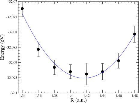
Figure 1: The potential energy curve of H₂ as obtained by AF QMC with a planewave basis and a hydrogen pseudopotential. We show also a Morse potential fit for the QMC data. The QMC equilibrium bondlength from the fit is 1.416(4) Bohr to be compared with the exact value is 1.40083 Bohr. Supercell used is $16\times 12\times 11$ Bohr³.

As mentioned, AF QMC relies on a trial wave function to control the phase problem. In the planewave calculations, we used a single Slater determinant from a planewave based density functional calculation obtained with a GGA functional gga , with no further optimizations.

III.1 Ortho- and Para-H₂ molecule

Table 1 summarizes results for the binding energy of the H₂ molecule, using DFT/GGA and AF QMC for several supercells, and compares these to exact results roothaan and experiment. The experimental bondlength of H₂ was used in all the calculations. The binding energy is calculated as the difference in energy between the H atom (times two) and the molecule, each placed in the same supercell. The density functional binding energy obtained using the hydrogen pseudopotential converges, with respect to size effect, to $4.531$ eV, which is in reasonable agreement with the all-electron (i.e. using the proton’s bare Coulomb potential) binding energy $4.568$ eV obtained using NWCHEM nwchem , and with the all-electron value of 4.540 eV reported in Ref. patton . The agreement between the pseudopotential and all-electron results is a reflection of the good transferability of the hydrogen pseudopotential. The AF QMC binding energy with the largest supercell is 4.74(2) eV, which is in excellent agreement with the experimental value of 4.75 eV (zero point energy removed) and the exact calculated value of 4.746 eV roothaan .

Figure 1 shows the H₂ AF QMC potential energy curve, using a $16\times 12\times 11$ Bohr³ supercell. Finite size effects, as in Table 1, likely vary with the H₂ bondlength and would affect the shape of the curve. Using a Morse potential fit, we obtained an estimated bondlength of $1.416(4)$ Bohr. (Using a 2nd or 4th order polynomial fit leads to similar results; with 4th order fit the error bar is three times larger). For comparison, the exact equilibrium bondlength of H₂ is $1.40083$ a.u roothaan , and the DFT/GGA bondlength is 1.4213 Bohr.

The energy difference between the ortho- and para-H₂ spin states (${}^{1}\Sigma$ and ${}^{3}\Sigma$, respectively) was also calculated. We note that for the singlet H₂ two-electron system, a HS transformation based on the magnetization Silvestrelli93 can be made to eliminate the sign problem and thus the need for the phaseless approximation. In this case the AF QMC calculations will become exact. This is not done here, since our goal is to benchmark the general algorithm. The calculations for both ortho- and para-H₂ were at the experimental bondlength of ortho H₂. Table 2 summarizes the results. The exact value obtained by Kolos and Roothaan is $10.495$ eV roothaan , with which the AF QMC value at the larger supercell size is in excellent agreement.

Table 2: Planewave based AF QMC energies of the ortho- (${}^{1}\Sigma$) and para-H₂ (${}^{3}\Sigma$) molecule for two supercell sizes. The bondlength was fixed at $R=1.42$ Bohr in all cases. All energies are in eV. The exact calculated energy gap $\Delta$ is $10.495$ eV roothaan . Statistical errors are on the last digit and are shown in parenthesis.

supercell	${}^{1}\Sigma$	${}^{3}\Sigma$	$\Delta$
11$\times$9$\times$7	$-$32.59(1)	$-$22.329(4)	10.26(1)
22$\times$18$\times$14	$-$32.01(2)	$-$21.546(7)	10.46(2)

III.2 H₂+H $\longrightarrow$ H+H₂ transition state

The problem of calculating the transition state of H₃ is well benchmarked using a variety of methods H3_siegbahn ; anderson_1994 ; anderson_2005 ; Peterson_H3 ; porezag_H3 . The activation energy for the reaction H₂+H $\longrightarrow$ H+H₂ is defined as the difference between the energy of the H₃ saddle point and that of the well separated H atom and H₂ molecule.

Density functional methods are not very accurate in calculating the activation energy. For example, DFT with an LDA functional gives H₃ as a bound molecule with a binding energy of $0.087$ eV at the symmetric configuration with $R_{1}=R_{2}=1.795$ Bohr. DFT/GGA, on the other hand, gives a barrier height of $0.152$ eV at the symmetric configuration $R=1.767$ Bohr porezag_H3 . The experimental barrier height is 9.7 kcal/mol$=0.420632$ eV H3_exp .

Table 3: Symmetric collinear H₃ transition state energies using planewaves with pseudopotentials. Results are shown from density functional GGA [with (PSP) and without (AE) pseudopotentials, respectively], DMC, and the present AF QMC methods. (The “all-electron” GGA(AE) results are from well converged large Gaussian basis set calculations.) The calculated results are for the linear H₃ molecule with $R_{1}=R_{2}=R$, for three values of $R$. All energies are in eV. Statistical errors are on the last digit and are shown in parenthesis.

R	GGA(AE)	GGA(PSP)	DMC (exact)	AF QMC
$1.600$	0.297	0.30	0.543 09(8)	0.54(3)
$1.757$	0.156	0.16	0.416 64(4)	0.43(3)
$1.900$	0.222	0.22	0.494 39(8)	0.48(4)

Using the AF QMC method, we studied the collinear H₃ system for three configurations with R₁=R₂=1.600, 1.757, and 1.900 Bohr. Table 3 shows the calculated barrier heights and compares these to results from DFT/GGA all-electron and pseudopotential calculations, and to results from recent DMC calculations anderson_2005 . The AE and pseudopotential DFT/GGA results are in excellent agreement with each other, a further indication of the good quality of the H pseudopotential. The DMC calculations anderson_2005 are exact in this case, through the use of a cancellation scheme FermionSign2 ; Anderson_cancel , which is very effective at eliminating the sign problem for small systems. The AF QMC values are in good agreement with the exact calculated results.

Planewave based AF QMC calculations of the H₃ transition state are very expensive, since the energy variations in the Born-Oppenheimer curve are quite small as seen in Table 3. To achieve the necessary accuracy, large supercells are needed, which results in large planewave basis sets. The large basis sets lead to many thousands of AF’s in Eq. (3). Moreover, a large number of AF’s in general lead to a more severe phase problem and thus potentially a more pronounced role for the phaseless approximation. The larger AF QMC statistical errors, compared to the highly optimized DMC results as well as to our Gaussian basis results in Sec. IV.2, reflect the inefficiency of planewave basis sets for isolated molecules. These calculations are valuable, despite their computational cost, as they demonstrate the robustness of the method.

III.3 Hydrogen-bonded molecules

Complementing the study above of the H₃ system, where energy differences are small, we also examined three other hydrogen-bonded molecules: H₂O, OH, and H₂O₂, where the energy scales are large. Table 4 compares the binding energies calculated using DFT/GGA (both pseudopotential and all-electron), DMC grossman , and the present AF QMC method. (Results for the O₂ and O₃ molecules are included, because they are pertinent to the discussion of pseudopotentials errors below.) The experimental values feller_peterson , with the zero point energy removed, are also shown. All of the calculations are performed at the experimental geometries of the molecules. The density functional all-electron binding energies in Table 4 were obtained using the highly converged triple-zeta ANO basis sets of Widmark, Malmqvist, and Roos roos . They are in good agreement with published all-electron results. For example, the all-electron binding energy of H₂O is 10.147 eV and that of OH is 4.77 eV in Ref. gga . In Ref. patton , the binding energy of H₂O is 10.265 eV, and that of O₂ is 6.298 eV patton .

In all of the molecules except H₂O, the DFT pseudopotential result seems to be in better agreement with the experimental value than the all-electron result. This is fortuitous and by no means suggest that the pseudopotential results are better than the all-electron values, since the pseudopotentials results should reproduce the all-electron value obtained with the same theory. Any differences are in fact due to transferability errors of the pseudopotentials. At the density functional level, the molecular systems H₂O, OH, and H₂O₂ all need a non-linear core correction (NLCC). The NLCC was introduced into DFT pseudopotential calculations by Louie et. al. nl_core . It arises from the DFT-generated pseudopotential for oxygen, at the pseudopotential construction level in the descreening step, where the valence Hartree and nonlinear exchange-correlation terms are subtracted to obtain the ionic pseudopotential. The Hartree term is linear in the valence charge and can be subtracted exactly. This is not the case with the nonlinear exchange-correlation potential, and will lead to errors especially when there is an overlap between the core and the valence charge densities. According to the NLCC correction scheme, this error can be largely rectified by retaining an approximate pseudo-core charge density, and carrying it properly in the target (molecular or solid) calculations. This generally improves the transferability of the pseudopotentials nl_core ; nl_core_porezag . The problem of NLCC is absent in effective core-potentials (ECP) generated using the Hartree-Fock method.

All of the molecules in Table 4 suffer from the NLCC error which originates predominantly from the spin-polarized oxygen atom, where the NLCC can be as large as $0.3$ eV/atom within a GGA-PBE calculation nl_core_porezag . For this reason, we have also included results for the O₂ and O₃ molecules. (The AF QMC value for O₂ is taken Ref. alsaidi_tio_mno .) As seen in the table, the binding energies of H₂O, OH, H₂O₂, O₂, and O₃ are smaller than the corresponding all-electron values by $\approx 0.37$, $0.19$, $0.60$, $0.50$, and $0.87$ eV, respectively. These values are approximately proportional to the number of oxygen atoms in the corresponding molecule with a proportionality constant $\approx 0.3$ eV, which agrees with the value reported in Ref. nl_core_porezag .

The pseudopotential is of course used differently in many-body AF QMC calculations. Despite the need for NLCC at the DFT level, the oxygen pseudopotential seems to be of good quality when used in AF QMC. In all the cases, the AF QMC results are in good agreement with DMC and with the experimental values. The largest discrepancy with experiment is $\approx 0.4(2)$ eV with O₃, and it is in opposite direction to the NLCC as done at the density functional level.

The need for the non-linear core correction does not indicate a failure of the frozen-core approximation, but rather is a consequence of the non-linear dependence of the spin-dependent exchange-correlation potential on the total spin-density (valence+core) in density functional theory. The QMC calculations depend only on the bare ionic pseudopotential and do not have this explicit dependence on the (frozen) core-electron spin densities. It is thus reasonable to expect the QMC results to be not as sensitive to this issue.

Table 4: Calculated binding energies of H₂O, OH, H₂O₂, O₂, and O₃. Results are shown from density functional GGA [with (PSP) and without (AE) pseudopotentials, respectively], DMC, and the present AF QMC methods. Experimental results are also shown. DFT/GGA(PSP) and the present AF QMC results were calculated using planewave basis sets with pseudopotentials. DFT/GGA(AE) is calculated using highly converged Gaussian basis sets. The DMC grossman results were also obtained using pseudopotentials. The zero point energy is removed from the experimental data feller_peterson . All energies are in eV. Statistical errors are on the last digit and are shown in parenthesis.

	GGA(AE)	GGA(PSP)	DMC	AF QMC	Expt.
H2O	10.19	9.82	10.10(8)	9.9(1)	10.09
OH	4.79	4.60	4.6(1)	4.7(1)	4.63
H2O2	12.26	11.66	11.4(1)	11.9(3)	11.65
O2	6.22	5.72		5.2(1)	5.21
O3	7.99	7.12		6.2(2)	5.82

Table 5: Symmetric collinear H₃ transition state total energies using aug-cc-pVDZ and aug-cc-pVTZ Gaussian basis sets dunning1 . We examined 5 configurations with $R_{1}=R_{2}=R$, and we report the unrestricted Hartree-Fock (UHF), full configuration interaction (FCI), and AF QMC total energies. Bondlengths are in Bohrs and energies are in Hartrees. Statistical errors are on the last digit and are shown in parenthesis.

R	UHF	FCI	AF QMC
aug-cc-pVDZ
1.600	$-1.595\,026$	$-1.642\,820$	$-1.642\,56(5)$
1.700	$-1.600\,252$	$-1.648\,186$	$-1.647\,75(5)$
1.757	$-1.601\,336$	$-1.649\,328$	$-1.648\,82(5)$
1.800	$-1.601\,406$	$-1.649\,433$	$-1.648\,98(6)$
1.900	$-1.599\,536$	$-1.647\,606$	$-1.646\,97(6)$
aug-cc-pVTZ
1.600	$-1.599\,843$	$-1.652\,219$	$-1.651\,78(7)$
1.700	$-1.604\,162$	$-1.656\,405$	$-1.655\,86(7)$
1.757	$-1.604\,835$	$-1.657\,013$	$-1.656\,52(7)$
1.800	$-1.604\,638$	$-1.656\,770$	$-1.656\,24(8)$
1.900	$-1.602\,269$	$-1.654\,285$	$-1.653\,68(9)$

IV Results using Gaussian basis sets

In this section, we present our studies using Gaussian basis sets. For comparison, some of the systems are repeated from the planewave and pseudopotential studies in the previous section. Gaussian basis sets are in general more efficient for isolated molecules. For example, the calculations below on the Van der Waals minimum in H₃ would be very difficult with the planewave formalism, because of the large supercells necessary, and because of the high statistical accuracy required to distinguish the small energy scales. Also, all-electron calculations are feasible with a Gaussian basis, at least for lighter elements, so systematic errors due to the use of pseudopotentials can be avoided without incurring much additional cost.

Direct comparison with experimental results requires large, well-converged basis sets in the AF QMC calculations gafqmc_postd ; gafqmc . As mentioned, the convergence of Gaussian basis sets is not as straightforward to control as that of planewaves. For benchmarking the accuracy of the AF QMC method, however, we can also compare with other established correlated methods such as full configuration interaction (FCI) and CCSD(T), since all the methods operate on the same Hilbert space. FCI energies are the exact results for the Hilbert space thus defined. The FCI method has an exponential scaling with the number of particles and basis size, so it is only used with small systems. In this section, we study H₂ and H₃, which are challenging examples for mean-field methods, and compare the AF QMC results with exact results.

The matrix elements which enter in the definition of the Hamiltonian of the system of Eq. (1) are calculated using NWCHEM nwchem ; gafqmc . The trial wave functions, which are used to control the phase problem, are mostly computed using unrestricted Hartree-Fock (UHF) methods, although we have also tested ones from density functional methods. In previous studies, we have rarely seen any difference in the AF QMC results between these two types of trial wave functions. This is the case for most of the systems in the present work, and only one set of results are reported. In H₃ near the Van der Waals minimum, where extremely small energy scales need to be resolved, we find small differences ($\sim$ 0.1 milli-Hartree), and we report results from the separate trial wave functions. The FCI calculations were performed using MOLPRO molpro ; fci_molpro .

IV.1 Bondlength of H₂

We first study H₂ again, with a cc-pVTZ basis set which has 28 basis functions for the molecule. This is to be compared with the planewave calculations which has about $5,000$ to $70,000$ planewaves for the different supercells used. These H-bonded systems are especially favorable for localized basis sets. The AF QMC equilibrium bondlength $R=1.4025(6)$ Bohr compares well to the corresponding FCI bondlength of $R=1.40265$ Bohr, with both methods using the cc-pVTZ basis. This is a substantially better estimate of the exact infinite basis result of $R_{e}=1.40083$ Bohr roothaan than was obtained from the planewave AF QMC results in Fig. 1. The remaining finite-basis error is much smaller than the statistical errors in the planewave calculations. (The small residual finite-basis error is mostly removed at the cc-pVQZ basis set level, with an equilibrium bondlength of $R=1.40111$ Bohr from FCI.)

Table 6: H₃ total energies in the van der Walls limit. $R_{1}$ is fixed at $1.4$ Bohr, and $R_{2}$ is varied between 4 and 10 Bohr. The aug-cc-pVTZ basis set is used. Energies are in Hartrees. Statistical errors are on the last digit and are shown in parenthesis.

$R_{2}$	FCI	AF QMC/UHF
4	$-1.671\,577$	$-1.671\,60(9)$
5	$-1.672\,455$	$-1.672\,50(8)$
6	$-1.672\,535$	$-1.672\,63(6)$
7	$-1.672\,508$	$-1.672\,65(5)$
10	$-1.672\,462$	$-1.672\,57(6)$

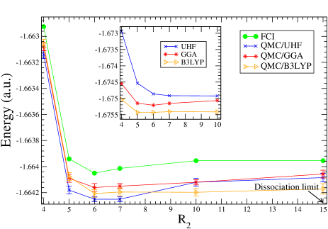
Figure 2: Potential energy curve of H₃ in the van der Waals limit using aug-cc-pVDZ basis set. $R_{1}$ is set to 1.4 Bohr, and $R_{2}$ is varied between 4 and 10 Bohrs. (The dissociation limit is shown at $R_{2}=15$ Bohr in the figure). FCI results are compared with AF QMC results with three different trial wave functions, from UHF and DFT with GGA and B3LYP functionals, respectively. The inset shows the corresponding potential energy curves obtained from UHF, GGA, and B3LYP. (For clarity, the UHF and GGA energies are shifted by $-0.047$ and $-0.154$ Hartrees in the inset, respectively.)

IV.2 H₂+H $\longrightarrow$ H+H₂ transition state

Table 5 presents calculated total energies of H₃ with aug-cc-pVDZ and aug-cc-pVTZ basis sets dunning1 . Results obtained with UHF, FCI, and the present AF QMC methods are shown for five different geometries in the collinear H₃ system. The present TZ-basis FCI results were cross-checked with those in Ref. Peterson_H3 , which contains a detailed study of the Born-Oppenheimer potential energy curves for the H+H₂ system.

The AF QMC total energies are in excellent agreement, to within less than 1 mE_H, with the FCI energies. The AF QMC barrier heights with the aug-cc-pVDZ and aug-cc-pVTZ basis sets at $R=1.757$ Bohr are 0.444(2) and 0.434(3) eV, respectively. The corresponding FCI results are 0.4309 and 0.4202 eV, respectively. Thus the AF QMC results show a systematic error of $\sim 0.015$ eV in the barrier height. It is possible to resolve these small discrepancies, because the basis sets are much more compact, with $25$ to $75$ Gaussian basis functions as opposed to approximately $10,000$ planewaves in the calculations in Sec. III.2. As a result, the statistical errors are smaller than in the planewave calculations by a factor of 10, with only a small fraction of the computational time. Even with these relatively small basis sets, we see that the finite-basis errors are quite small here. In fact, the FCI barrier height with the aug-cc-pVTZ basis is in agreement with the experimental value 0.420632 eV H3_exp .

IV.3 Van der Waals minimum in collinear H₃

The van der Waals minimum of H₃ is studied by fixing $R_{1}=1.4$ Bohr (the H₂ equilibrium bond length), while the distance $R_{2}$ between the third H atom and the closer of the two atoms in H₂ was varied between $4$ and $10$ Bohrs. The potential energy curve of this system exhibits a very shallow minimum of approximately $85\,\mu$E_H Peterson_H3 at $R_{2}\sim 6$ Bohr. Two different basis sets, aug-cc-pVDZ and aug-cc-pVTZ, were used. Table 6 shows the aug-cc-pVTZ results, and Fig. 2 plots the aug-cc-pVDZ results.

As seen in Table 6, the AF QMC all-electron total energies are in excellent agreement with FCI, with a maximum discrepancy of about $0.14(5)$ mE_H. The AF QMC energies, which are calculated with the mixed-estimator, are not variational, as is evident in the results from both basis sets compared to FCI. The AF QMC results in Table 6 are obtained with an UHF trial wave function. In most of our molecular calculations with Gaussian basis sets, the UHF solution, which is the variationally optimal single Slater determinant, has been chosen as the trial wave function gafqmc ; gafqmc_postd . In the present case, the UHF method actually fails to give a Van der Waals minimum, as can be seen from the inset of Fig. 2. It is reassuring that AF QMC correctly reproduces the minimum with UHF as a trial wave function.

The effects of using two other single Slater determinant trial wave functions were also tested. These were obtained from DFT GGA and B3LYP calculations with the aug-cc-pVDZ basis set. The corresponding results are also shown in Fig. 2. In the DFT calculations (shown in the inset of Fig. 2), both GGA and B3LYP predict the existence of a minimum, although B3LYP gives an unphysical small barrier at about $R_{2}\approx 7$ Bohr. The AF QMC results obtained with UHF, GGA, and B3LYP Slater determinants as trial wave functions differ somewhat, but are reasonably close to each another. With the GGA trial wave function, AF QMC “repairs” the well depth (possibly with a slight over-correction). With the B3LYP trial wave function, AF QMC appears to under-estimate the well-depth, giving a well-shape that is difficult to characterize because of the statistical errors and the extremely small energy scale of these features.

V Summary

We have presented a benchmark study of the phaseless AF QMC method in various H-bonded molecules. The auxiliary-field QMC method is a many-body approach formulated in a Hilbert space defined by a single-particle basis. The choice of a basis set is often of key importance, as it can affect the efficiency of the calculation. In the case of AF QMC, the basis set choice can also affect the systematic error, because of the different HS transformation that can result. In this study, we employed planewave basis sets with pseudopotentials and all-electron Gaussian basis sets, to compare the performance of the AF QMC method. The planewave HS decomposition was tailored to the planewave representation, resulting in ${\mathcal{O}}(8~{}M)$ auxiliary fields, where $M$ is the number of planewaves. For the Gaussian basis sets, the generic HS decomposition described in Section II was used, resulting in ${\mathcal{O}}(M^{2})$ auxiliary fields. Typical $M$ values in this study were tens of thousands in the planewave calculations and a hundred in the Gaussian calculations.

The planewave calculations were carried out for H₂, ${\rm H}_{2}+{\rm H}$ near the transition state, H₂O, OH, and H₂O₂. Non-linear core corrections to the oxygen pseudopotential were discussed using additional calculations for the O₂ and O₃ molecules. DFT GGA pseudopotentials were employed. The trial wave functions were single Slater determinants obtained from DFT GGA with identical planewave and pseudopotential parameters as in the AF QMC calculations. Hard pseudopotentials and large planewave cutoffs were used to ensure basis-size convergence and the transferability of the pseudopotentials. Large supercells were employed to remove finite-size errors. To mimic typical systems in the solid state, no optimization was done to take advantage of the simplicity of these particular systems. The binding energies computed from AF QMC have statistical errors of 0.1-0.3 eV as a result. Within this accuracy, the AF QMC results are in excellent agreement with experimental values.

Gaussian basis AF QMC calculations were carried out on H₂, the transition state of ${\rm H}_{2}+{\rm H}$, as well as the van der Waals minimum in linear ${\rm H}_{2}+{\rm H}$. These calculations are within the framework of standard quantum chemistry many-body using the full Hamiltonian without pseudopotentials. UHF single Slater determinants were used as the trial wave function. For various geometries, the absolute total energies from AF QMC agree with FCI to well within 1 mE_H. The calculated equilibrium bondlengths and potential energy curves are also in excellent agreement with FCI. In ${\rm H}_{2}+{\rm H}$, AF QMC correctly recovers the van der Waals well with a UHF trial wave function which in itself predicts no binding.

Comparing planewave and Gaussian basis set AF QMC results, we can conclude the following. In the Gaussian basis calculations, as evident from FCI comparisons, errors due to controlling the phase problem in the phaseless approximation are well within 1 mE_H in the absolute energies. Achieving the infinite basis limit is more straightforward using planewave based AF QMC, but statistical errors are larger for the isolated molecules studied due to the need for large supercells. Within statistical errors, however, the AF QMC results using both types of basis sets were in agreement. This indicates that errors due to the use of pseudopotentials with planewave basis sets were smaller than the statistical errors. Finally, within statistical errors, the performance of the phaseless AF QMC method, did not appear to be sensitive to the type of HS decomposition used, despite drastic differences in basis size and the number of auxiliary fields. was tailored

VI Acknowledgments:

We would like to thank E. J. Walter for many useful discussions. This work is supported by ONR (N000140110365 and N000140510055), NSF (DMR-0535529), and ARO (grant no. 48752PH). Computations were carried out in part at the Center for Piezoelectrics by Design, the SciClone Cluster at the College of William and Mary, and NCSA at UIUC supercomputers.

References

- (1) W. M. C. Foulkes, L. Mitas, R. J. Needs, and G. Rajagopal, Rev. Mod. Phys. 71, 33 (2001).
- (2) S. Zhang and H. Krakauer, Phys. Rev. Lett. 90, 136401 (2003).
- (3) W. A. Al-Saidi, S. Zhang, and H. Krakauer, J. Chem. Phys. 124, 224101(2006).
- (4) M. C. Payne, M. P. Teter, D. C. Allan, T. A. Arias and J. D. Joannopoulos, Rev. Mod. Phys. 64, 1045 (1992).
- (5) A compilation of basis sets is present at the Extensible Computational Chemistry Environment Basis Set Database (http://www.emsl.pnl.gov/forms/basisform.html).
- (6) T. H. Dunning, Jr., J. Chem. Phys. 90, 1007 (1989).
- (7) D. E. Woon and T. H. Dunning, Jr, J. Chem. Phys. 98, 1358 (1993).
- (8) D. M. Ceperley and B. J. Alder, J. Chem. Phys. 81, 5833 (1984); J. B. Anderson in Quantum Monte Carlo: Atoms, Molecules, Clusters, Liquids and Solids, Reviews in Computational Chemistry, Vol. 13, ed. by Kenny B. Lipkowitz and Donald B. Boyd (1999).
- (9) Shiwei Zhang and M. H. Kalos, Phys. Rev. Lett. 71, 2159 (1993)
- (10) Shiwei Zhang, J. Carlson, and J. E. Gubernatis, Phys. Rev. B 55, 7464 (1997).
- (11) J. B. Anderson, J. Chem. Phys. 63, 1499 (1975).
- (12) J. W. Moskowitz, K. E. Schmidt, M. A. Lee, and Malvin H. Kalos, J. Chem. Phys. 77, 349 (1982); Peter J. Reynolds, David M. Ceperley, B. J. Alder, and W. A. Lester, J. Chem. Phys. 77, 5593 (1982).
- (13) W. A. Al-Saidi, H. Krakauer, and S. Zhang, Phys. Rev. B 73, 075103 (2006).
- (14) W. A. Al-Saidi, H. Krakauer, and S. Zhang, J. Chem. Phys. 125, 154110 (2006).
- (15) W. A. Al-Saidi, H. Krakauer, and S. Zhang, in preparation.
- (16) R. L. Stratonovich, Sov. Phys. Dokl. 2, 416 (1958); J. Hubbard, Phys. Rev. Lett. 3, 77 (1959).
- (17) T. P. Straatsma, E. Aprá, T. L. Windus, E. J. Bylaska, W. de Jong, S. Hirata, M. Valiev, M. T. Hackler, L. Pollack, R. J. Harrison, M. Dupuis, D. M. A. Smith, J. Nieplocha, V. Tipparaju, M. Krishnan, A. A. Auer, E. Brown, G. Cisneros, G. I. Fann, H. Fruchtl, J. Garza, K. Hirao, R. Kendall, J. A. Nichols, K. Tsemekhman, K. Wolinski, J. Anchell, D. Bernholdt, P. Borowski, T. Clark, D. Clerc, H. Dachsel, M. Deegan, K. Dyall, D. Elwood, E. Glendening, M. Gutowski, A. Hess, J. Jaffe, B. Johnson, J. Ju, R. Kobayashi, R. Kutteh, Z. Lin, R. Littlefield, X. Long, B. Meng, T. Nakajima, S. Niu, M. Rosing, G. Sandrone, M. Stave, H. Taylor, G. Thomas, J. van Lenthe, A. Wong, and Z. Zhang, “NWChem, A Computational Chemistry Package for Parallel Computers, Version 4.6” (2004), Pacific Northwest National Laboratory, Richland, Washington 99352-0999, USA.
- (18) W. Kolos and C. C. J. Roothaan, Rev. Mod. Phys. 32, 219 (1960).
- (19) Andrew M. Rappe, Karin M. Rabe, Efthimios Kaxiras, and J. D. Joannopoulos, Phys. Rev. B 41, R1227 (1990).
- (20) Shiwei Zhang, Henry Krakauer, Wissam Al-Saidi, and Malliga Suewattana, Comp. Phys. Comm. 169, 394 (2005).
- (21) Malliga Suewattana, W. Purwanto, S. Zhang, H. Krakauer, and E. J. Walter (unpublished).
- (22) Steven G. Louie, Sverre Froyen, and Marvin L. Cohen Phys. Rev. B 26, 1738 (1982).
- (23) Dirk Porezag, Mark R. Pederson, and Amy Y. Liu , Phys. Rev. B 60, 14132 (1999).
- (24) J. P. Perdew, K. Burke, and M. Ernzerhof, Phys. Rev. Lett 77, 3865 (1996).
- (25) David C. Patton, Dirk V. Porezag, and Mark R. Pederson, Phys. Rev. B 55, 7454 (1996).
- (26) P. L. Silvestrelli, S. Baroni, and R. Car, Phys. Rev. Lett. 71, 1148 (1993).
- (27) P. Siegbahn and B. Liu, J. Chem. Phys. 68, 2457 (1978).
- (28) Drake L. Diedrich and James B. Anderson, J. Chem. Phys. 100, 8089 (1994).
- (29) Kevin E. Riley and James B. Anderson, J. Chem. Phys. 118, 3437 (2002).
- (30) Steven L. Mielke, Bruce C. Garrett, and Kirk A. Peterson, J. Chem. Phys. 116, 4142 (2001).
- (31) Dirk Porezag and Mark R. Pederson, J. Chem. Phys. 102, 9345 (1995).
- (32) W. R. Schulz and D. J. Le Roy, J. Chem. Phys. 42, 3869 (1965).
- (33) J. B. Anderson, C. A. Traynor, and B. M. Boghosian, J. Chem. Phys. 95, 7418 (1991).
- (34) Jeffery C. Grossman, J. Chem. Phys. 117, 1434 (2002).
- (35) David Feller, and Kirk A. Peterson, J. Chem. Phys. 110, 8384 (2002).
- (36) P. O. Widmark, P. A. Malmqvist, and B. Roos, Theo. Chim. Acta, 77, 291 (1990).
- (37) MOLPRO version 2002.6 is a package of ab initio programs written by H.-J. Werner and P. J. Knowles, with contributions from J. Almlof, R. D. Amos, M. J. O. Deegan, S. T. Elbert, C. Hampel, W. Meyer, K. A. Peterson, R. M. Pitzer, ¨ A. J. Stone, P. R. Taylor, and R. Lindh, Universitat Bielefeld, Bielefeld, Germany, University of Sussex, Falmer, Brighton, England, 1996.
- (38) P. J. Knowles and N. C. Handy, Chem. Phys. Letters 111, 315 (1984); P. J. Knowles and N. C. Handy, Comp. Phys. Commun. 54, 75 (1989).