Yet on statistical properties of traded volume: correlation and mutual information at different value magnitudes

Abstract

In this article we analyse linear correlation and non-linear dependence of traded volume, $v$, of the $30$ constituents of Dow Jones Industrial Average at different value scales. Specifically, we have raised $v$ to some real value $\alpha$ or $\beta$, which introduces a bias for small ($\alpha,\,\beta<0$) or large ($\alpha,\,\beta>1$) values. Our results show that small values of $v$ are regularly anti-correlated with values at other scales of traded volume. This is consistent with the high liquidity of the $30$ equities analysed and the asymmetric form of the multi-fractal spectrum for traded volume which has supported the dynamical scenario presented by us.

I Introduction

Financial market analysis has become one of the most significative examples about application of concepts associated with physics to systems that are usually studied by other sciences bouchaud-potters-book . In this sense, ideas like scale invariance and cooperative phenomena have also found significance in systems that are not described neither by some Hamiltonian nor some other kind of equation usually associated with Physics (e.g., a master equation). Although plenty of work has been made on the analysis and mimicry of price fluctuations, less attention has been paid to an important observable intimately related to changes in price, the traded volume, $v$ karpoff . In fact, traded volume has been coupled to price fluctuations both on an empirical or analytical way for some time early . Nonetheless, a consistent analysis of intrinsic statistical properties of traded volume appears to be first presented in Reference gopi-volume . Thereafter, it has been enlarged or revisited by different authors vol-anal ; eisler ; creta ; bariloche . In this article, we apply a generalisation of the traditional linear self-correlation function in order to study how small, large, and about average (frequent) values of $v$ relate between them in time. Furthermore, we analyse non-linear dependence using a generalised measure based on Kulback-Leibler mutual information. Our data set is made up of 1 minute traded volume time series, running from the $1^{st}$ July 2004 to the $31^{st}$ December 2004, for the $30$ equities that make the Dow Jones Industrial Average index. Aiming to avoid the well-known intraday profile, traded volume time series were previously treated according to a standard procedure (see e.g. bariloche ).

II Generalised linear self-correlation function

The (normalised) correlation function, generally,

$$C\left(A\left(\vec{r},t\right),B\left(\vec{r}^{\prime},t^{\prime}\right)\right)=\frac{\left\langle A\left(\vec{r},t\right)\,B\left(\vec{r}^{\prime},t^{\prime}\right)\right\rangle-\left\langle A\left(\vec{r},t\right)\right\rangle\left\langle B\left(\vec{r}^{\prime},t^{\prime}\right)\right\rangle}{\sqrt{\left\langle A\left(\vec{r},t\right)^{2}\right\rangle-\left\langle A\left(\vec{r},t\right)\right\rangle^{2}}\sqrt{\left\langle B\left(\vec{r}^{\prime},t^{\prime}\right)^{2}\right\rangle-\left\langle B\left(\vec{r}^{\prime},t^{\prime}\right)\right\rangle^{2}}},$$ (1)

represents a useful analytical form to evaluate how much two random variables depend, linearly, on each other. Leaving out spatial dependence, when $A$ and $B$ are the same observable, Eq. (1) represents the straightforwardest way to appraise memory in the evolution of $A$. In any case, it does not give us any information about the role of magnitudes. Inspired by multi-fractal analysis scaling , a simple way to quantify this type of correlation can be defined by introducing a generalised self-correlation function, $C\left(\hat{A}\left(t\right),\tilde{A}\left(t^{\prime}\right)\right)\equiv C_{\alpha,\beta}\left(A\right)$, where $\hat{A}\left(t\right)=\left|A\left(t\right)\right|^{\alpha}$, $\tilde{A}\left(t\right)=\left|A\left(t\right)\right|^{\beta}$ (with $\alpha,\beta\neq 0$ $\in\Re$), and $t^{\prime}=t+\tau$ . As an example let us assume $\beta=1$. For values of $\alpha$ greater than $1$, small values of $A$ become even smaller and their weight in the value of $C_{\alpha,\beta}\left(A\right)$, due to $\hat{A}\left(t\right),\tilde{A}\left(t^{\prime}\right)$, approaches negligibility (e.g., when $\alpha=2$, $v=10^{-1}>v^{\alpha}=10^{-2}$ and $v=10<v^{\alpha}=10^{2}$). Otherwise, when $\alpha$ is negative, we highlight values around zero (e.g., when $\alpha=-1$, $v=10^{-1}<v^{\alpha}=10^{1}$ and $v=10>v^{\alpha}=10^{-1}$). In the end, after summing over all pairs $\left(\hat{A}\left(t\right),\tilde{A}\left(t^{\prime}\right)\right)$, we verify that the main contribution for $C_{\alpha,1}\left(A\right)$ comes from large values of $\left|A\left(t\right)\right|$ when $\alpha>1$ and from small values of $\left|A\left(t\right)\right|$ when $\alpha<0$. Accordingly, for $\alpha=\beta$, we estimate how values of the same order of magnitude are related in time, when $\alpha\neq\beta$ we analyse the relation between values with different magnitudes.

In Fig. 1 we depict the results that we have obtained by applying Eq. (1), with different pairs of $\left(\alpha,\beta\right)$ in traded volume time series. In Table 1 we present the values of the numerical adjustment of $C_{\alpha,\beta}\left(A\right)$ for a double exponential function,

$$f\left(x\right)=a\exp\left[-\frac{x}{\tau_{1}}\right]+b\exp\left[-\frac{x}{\tau_{2}}\right].$$

We have set as minimum and maximum values for the exponents $-1$ and $2$. Our choice is justified by the fact they are both able to evaluate the influence of small and large values of $v$, and to preserve a reliable statistics.

From the analysis of figures in Table 1, we observe that small values, $\alpha(\beta)=-1$, are always anti-correlated with both frequent ($\alpha(\beta)=1$), and large ($\alpha(\beta)=2$) values of traded volume. We verify that there is temporal symmetry, which can be checked if we change $\alpha\leftrightarrow\beta$. When $\alpha$($\beta$) equal $-1$, the second scale of relaxation is consistently much larger than the observed when both exponents are positive. In addition, the values for coefficients $a$ and $b$ (in modulus) are smaller when at least one of the exponents is $-1$. This indicates that, besides presenting a negative influence over frequent and large values of $v$, such an influence is restrictable. On the other side, we have observed a very fast first decay of the correlation function for $\beta=2$ and $\alpha=1,2$ followed by a slower decay, though faster when compared with $\alpha=\beta=1$. This might be interpreted as a consequence of the low frequency in large values of $v$. This richness and disparity in behaviour for small and large values is congruous with a previous multi-fractal analysis of $v$ bariloche . In this analysis, it has been observed a strong asymmetry in multi-fractal spectrum, that has been associated with the existence of different dynamical mechanisms prompting small and large values for trading volume creta ; volume .

Table 1: Values of the parameters of adjust of $C_{\alpha,\beta}\left(A\right)$ for a double exponencial, $f\left(x\right)=a\exp\left[-\frac{x}{\tau_{1}}\right]+b\exp\left[-\frac{x}{\tau_{2}}\right]$ for the results presented on the panels of Fig. 1.

$\alpha$	$\beta$	$a$	$\tau_{1}$	$b$	$\tau_{2}$	$\chi^{2}$	$R^{2}$
$-1$	$-1$	$0.052\pm 0.001$	$29\pm 4$	$0.015\pm 0.002$	$1138\pm 11$	$2.0\times 10^{-5}$	$0.78$
$-1$	$1$	$-0.030\pm 0.001$	$37\pm 1$	$-0.027\pm 0.002$	$1526\pm 22$	$1.5\times 10^{-6}$	$0.97$
$-1$	$2$	$-0.004\pm 0.001$	$94\pm 9$	$-0.008\pm 0.001$	$1628\pm 17$	$5.8\times 10^{-7}$	$0.84$
$1$	$1$	$0.128\pm 0.002$	$27\pm 1$	$0.111\pm 0.001$	$844\pm 7$	$2.0\times 10^{-5}$	$0.99$
$1$	$2$	$0.102\pm 0.002$	$11\pm 1$	$0.050\pm 0.001$	$488\pm 4$	$6.5\times 10^{-6}$	$0.97$
$2$	$2$	$0.165\pm 0.002$	$4\pm 1$	$0.030\pm 0.001$	$354\pm 5$	$4.7\times 10^{-6}$	$0.96$

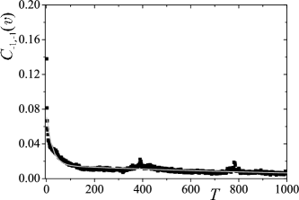
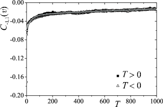
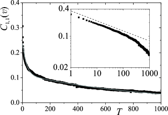
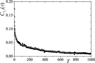
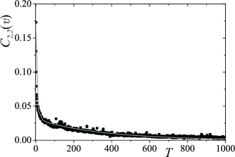
Figure 1: $C_{\alpha,\beta}(v)$ vs. $T$ for the values of $\alpha$ and $\beta$ presented in Table 1 (clockwise). On each panel black symbols are the values obtained from time series and the grey line represents the numerical fit of $C_{\alpha,\beta}(v)$ for a double exponential. In panel for $C_{-1,1}(v)$ the curves for $T>0$ and $T<0$ concur, which goes along the lines of time symmetry. The inset on $C_{1,1}(v)$ panel is a log-log representation of the main panel. As it is visible the correlation function does not present power-law behaviour. The same happens for all the other values of $(\alpha,\beta)$ studied.

III Generalised mutual information applied to DJ30 traded volume time series

In information theory, the Kullback-Leibler (KL) mutual information kullback-leibler-entropy (or information gain, or information divergence) is a distance measure (but not a metric distance) that provides the mean change of information related to any two probability distributions, $p$ and $p^{\prime}$. If we have, say, two experiments, with a given set of discrete outcoming probability distributions $p$ and $p^{\prime}$, respectively, then, the KL mutual information might be defined as,

$$K(p,p^{\prime})\equiv-\sum_{j}p_{j}\ln\frac{p_{j}^{\prime}}{p_{j}},$$ (2)

where $p_{j}$ ($p_{j}^{\prime}$) is the probability of outcome $j$ in experiment one (two). As a special case, we consider two random variables $x$ and $y$ and we set $p$ to be the joint probability distribution, $p=p(x,y)$ and $p^{\prime}$ the product of the marginal probability distributions, $p^{\prime}=p_{1}(x)p_{2}(y)$. In this particular case, the KL mutual information is usually referred to as mutual information (we will denote it as $I(x,y)$) and it is a useful and natural tool to measure the degree of statistical dependence between two random variables also applied in financial analysis tugas .

When considering traded volume, and since we are dealing with correlated non-linear processes, a natural way of generalising the KL mutual information can be achieved by replacing the usual statistical theory for the non-extensive statistical theory tsallis . In this generalisation, the usual logarithm must be replaced by the $q$-logarithm, defined as $\ln_{q}x=\frac{x^{1-q}-1}{1-q}$. When $q\rightarrow 1$, the $q$-logarithm becomes the usual one.

For $q>0$, there exist well defined minimum and maximum values of $I_{q}(p,p^{\prime})$ corresponding to minimum and maximum dependence degrees between random variables, e.g., $x$ and $y$. This allows us to define a criterion for statistical testing borland-plastino-tsallis through the normalised quantity $R\equiv\frac{I_{q}}{I_{q}^{max}},\,\in[0,1]$. Its extreme value $R=0$ ($R=1$) corresponds to zero (full) dependence between $x$ and $y$. Given $x$ and $y$, the ratio $R$ can be calculated as a function of $q$. Typically, $R$ varies smoothly and monotonically from 0 to 1, its two limiting values. The inflexion point in $R(q)$ determines the value of $q$ for which $R$ most sensibly detects changes in the correlation between $x$ and $y$. We call this value of $q$ as optimal value, $q^{op}$. It can be seen borland-plastino-tsallis that for one-to-one dependence we have $q^{op}=0$, and $q^{op}=\infty$ for total independence.

The generalised mutual information $R$ has already been used in creta applied to traded volume time series from the components of the Dow Jones 30 index. In order to compare this quantity with the self-correlation function, we have considered $x$ to be the time series and $y$ the same time series with a lag in time, $\tau\equiv T$. Here, we have further analysed this data by performing this calculation on the same lines as in section 1, i.e., we have defined our random variables by modifying the (normalised detrended) traded volume $v$ through exponents $\alpha$ and $\beta$, i.e., $x_{\alpha}=v_{j}^{\alpha}$ and $y_{\beta}=v_{j}^{\beta}$. Then, we have computed $R$ with the same exponents as in the section II. Our procedure can be summarised as follows: We have first derived the probability distributions for each component time series $i$ and its lagged counterpart with lag $\tau$. To construct the PDFs, we have set the bin size (or, in physics terms, the coarse-graining) to be $\Delta x=\Delta y=0.02,\forall i$. We then have calculated $R_{i}$ as a function of the index $q$. From this, we have extracted an optimal index $q_{i}^{op}(\tau,\alpha,\beta)$ for each component $i$. Finally, we have computed the mean $q^{op}$ value from all 30 components, i.e. $q^{op}=\frac{1}{30}\sum_{i=1}^{30}q_{i}^{op}(\tau,\alpha,\beta)$ .

In Fig. 2 we present our results for different values of $\alpha$ and $\beta$. Firstly we plot, for comparison purposes, the unmodified case $\alpha=1,\beta=1$ (panel $a$). There is a clear logarithmic dependence of $q^{op}$ as a function of the lag $\tau$. In the same panel we plot our results for $\alpha=2,\beta=1$, and its symmetric case $\alpha=1,\beta=2$. We obtain again a logarithmic behaviour, but both additive and multiplicative fitting parameters change. The rate of change is higher indicating that this particular choice of $\alpha$ and $\beta$ accelerates the loss of dependence in time. For $\alpha=1,\beta=2$, the multiplicative parameter is very close to $\alpha=2,\beta=1$ case (see caption), reflecting the same kind of symmetry observed in the section II. In panel $c$ we present results where $\alpha>0,\beta<0$ or $\alpha<0,\beta>0$. Our results show that, in this case, $q^{op}$ diminishes as a function of the lag, but the rate of change is not as high as in the $\alpha>0,\beta>0$ case (see caption). Note that this result occurs for the same exponents where anti-correlated behaviour is found (section II) suggesting that anti-correlation might imply on negative slope in the logarithmic behaviour. This possibility will be verified in future work, namely on the analysis of the dependence between volatility and traded volume progress .

To further analyse the meaning of these results, we have performed the same calculations on a shuffled version of the same time series, i.e. applying a random reordering (in time) on each component time series. We show our results in Fig. 2, panels $b$ and $d$, where we have use the same exponents as in panels $a$ and $c$ respectively. This shuffling procedure destroys causality and in every case $q^{op}$ looses its dependence with $\tau$. In all cases, the curves obtained from the unshuffled data evolve towards the shuffled ones, probably reaching them for high values of $\tau$. Thus, one can consider that $q^{op}$ obtained from the shuffled time series act as saturation values of the unshuffled case, when all dependence is lost.

Figure 2: Optimal index $q^{op}$ versus lag $\tau$. Panel $a$: Lines correspond to fitting function $q^{op}=A+B\log\tau$, where ($A,B$) is ($1.667\pm 0.003,0.035\pm 0.001$) (solid line), ($1.563\pm 0.004,0.035\pm 0.001$) (dashed line) and ($1.583\pm 0.001,0.0223\pm 0.0003$) (dotted line) for ($\alpha,\beta$)= (2,1), (1, 2) and (1, 1) respectively. Panels $b$: Same as in $a$ on the shuffled version of the time series. Constant values are: $1.954\pm 0.002$ (solid line), $1.858\pm 0.001$ (dashed line) and $1.7713\pm 0.0008$ (dotted line). Panel $c$: Logarithmic fitting as in $a$: ($A,B$) is ($1.977\pm 0.004,-0.007\pm 0.001$) (solid line), ($1.974\pm 0.008,-0.009\pm 0.002$) (dashed line), ($2.07\pm 0.01,-0.004\pm 0.002$) (dotted line) for ($\alpha,\beta$)= (2,-1), (1, -1) and (-1, 1) respectively. Panel $d$: Same as in $c$ on the shuffled version of the time series. Constant values are: $1.881\pm 0.002$ (solid line), $1.869\pm 0.002$ (dashed line) and $1.953\pm 0.005$ (dotted line).

IV Final remarks

To conclude, we have applied a generalised form of correlation function, $C_{\alpha,\beta}(.)$, in order to evaluate how values having different magnitudes influence each other. The results obtained point out that small values of traded volume are consistently anti-correlated with frequent and large values. Moreover, frequent and large values are positively correlated. These results are in accordance with the strong asymmetry of the multi-fractal spectrum, which has supported our dynamical scenario for the observable creta ; volume .

We also have investigated the effect of modifying our data through $\alpha$ and $\beta$ on the Kullback-Leibler generalised mutual information, and its associated optimal index $q^{op}$. Our results show that there is a logarithmic dependence of $q^{op}$ with lag in the positive exponents case ($\alpha>0,\beta>0$), with different fitting parameters depending on these exponents. In the case of negative $\alpha$ or $\beta$, we have observed that $q^{op}$ diminishes with lag. A further analysis on this intriguing behaviour is certainly welcome.

We thank C. Tsallis for several conversations on the subjects treated along this manuscript. SMDQ aknowledges previous discussions about multi-scaling with E. M. F. Curado and F. D. Nobre, and Z. Eisler for has provided some of the results in manuscript of Ref. eisler-com . We also thank Olsen Data Services for the data provided and used herein. LGM is thankful to the International Christian University in Tokyo for the warm hospitality. Financial support from FCT/MCES (Portuguese agency) and infrastructural support from PRONEX/CNPq (Brazilian agency) are also acknowledged.

References

- (1) J.-P. Bouchaud and M. Potters, Theory of Financial Risks: From Statistical Physics to Risk Management (Cambridge University Press, Cambridge, 2000); R.N. Mantegna and H.E. Stanley, An introduction to Econophysics: Correlations and Complexity in Finance (Cambridge University Press, Cambrigde, 1999); J. Voit, The Statistical Mechanics of Financial Markets (Springer-Verlag, Berlin, 2003)
- (2) J.M. Karpoff, J. Finan. Quantitat. Anal. 22, 109 (1997)
- (3) M.F.M. Osborne, Oper. Res. 7, 145 (1959); C.J.W. Granger and O. Morgenstern, Kyklos 16 (1), 1 (1963); C.C. Ying, Econometrica 34, 676 (1966)
- (4) P. Gopikrishnan, V. Plerou, X. Gabaix, and H.E. Stanley, Phys. Rev. E 62, R4493 (2000)
- (5) R. Osorio, L. Borland and C. Tsallis in: non-extensive Entropy - Interdisciplinary Applications, edited by: M. Gell-Mann and C. Tsallis (Oxford University Press, New York, 2004)
- (6) Z. Eisler and J. Kertész, Eur. Phys. J. B 51, 145 (2006)
- (7) J. de Souza, L.G. Moyano, and S.M. Duarte Queirós, Eur. Phys. J. B 50, 165 (2006)
- (8) L.G. Moyano, J. de Souza, and S.M. Duarte Queirós, Physica A 371, 118 (2006)
- (9) J. Feder, Fractals (Plenum, New York, 1988); A.-L. Barabási and T. Vicsek, Phys. Rev. A 44, 2730 (1991); M. Pasquini and M. Serva, Econ. Lett. 65, 275 (1999)
- (10) S.M. Duarte Queirós, Europhys. Lett. 71, 339 (2005)
- (11) S. Kullback and R.A. Leibler, Ann. Math. Stat. 22, 79 (1961)
- (12) C. Granger and J. Lin., J. Time Ser. Anal. 15, 371 (1994); A. Dionisio, R. Menezes and D.A. Mendes, Physica A 344, 326 (2004)
- (13) C. Tsallis, J. Stat. Phys. 52, 479 (1988); Related bibliography at: http://tsallis.cat.cbpf.br/biblio.htm
- (14) C. Tsallis, Phys. Rev. E 58, 1442 (1998)
- (15) L. Borland, A.R. Plastino and C. Tsallis, J.Math. Phys. 39, 6490 (1998); [Erratum: J. Math. Phys. 40, 2196 (1999)]
- (16) Z. Eisler, private communication on manuscript: Z. Eisler and J. Kertész, arXiv:physics/0606161 (preprint, 2006)
- (17) S.M. Duarte Queirós and L.G. Moyano, work in progress.