Scattering loss in electro–optic particulate composite materials

Tom G. Mackay^a and Akhlesh Lakhtakia^b

^aSchool of Mathematics
James Clerk Maxwell Building
University of Edinburgh
Edinburgh EH9 3JZ, United Kingdom
email: T.Mackay@ed.ac.uk

^bCATMAS — Computational & Theoretical Materials Sciences Group
Department of Engineering Science & Mechanics
212 Earth & Engineering Sciences Building
Pennsylvania State University, University Park, PA 16802–6812, USA
email: akhlesh@psu.edu

The effective permittivity dyadic of a composite material containing particulate constituent materials with one constituent having the ability to display the Pockels effect is computed, using an extended version of the strong–permittivity–fluctuation theory which takes account of both the distributional statistics of the constituent particles and their sizes. Scattering loss, thereby incorporated in the effective electromagnetic response of the homogenized composite material, is significantly affected by the application of a low–frequency (dc) electric field.

Keywords: Strong–permittivity–fluctuation theory, Pockels effect, correlation length, particle size, potassium niobate

1 Introduction

Two (or more) materials, each composed of particles which are small compared to all relevant wavelengths, may be blended together to create an effectively homogeneous material. By judiciously selecting the constituent materials, as well their relative proportions, particle shapes, orientations and sizes, and distributional statistics, the homogenized composite material (HCM) can be made to display desirable magnitudes of effective constitutive parameters [1, 2]. Furthermore, an HCM can exhibit effective constitutive parameters which are either not exhibited at all by its constituent materials, or at least not exhibited to the same extent by its constituent materials [3, 4]. A prime example of such metamaterials is provided by HCMs which support electromagnetic planewave propagation with negative phase velocity [5].

The focus of this paper is on the electromagnetic constitutive properties of HCMs [1, 6]. If one (or more) of the constituent materials exhibits the Pockels effect [7], then a further degree of control over the electromagnetic response properties of an HCM may be achieved. That is, post–fabrication dynamical control of an HCM’s performance may be achieved through the application of a low–frequency (dc) electric field. For such an HCM, the potential to engineer its electromagnetic response properties (i) at the fabrication stage by selection of the constituent materials and particulate geometry, and (ii) at the post–fabrication stage by an applied field, is of considerable technological importance in the area of smart materials [8].

The opportunities offered by the Pockels effect for tuning the response properties of composite materials have recently been highlighted for photonic band–gap engineering [9, 10] and HCMs [11]. In particular, the predecessor study exploiting the well–known Bruggeman homogenization formalism revealed that the greatest degree of control over the HCM’s constitutive parameters is achievable when the constituent materials are distributed as oriented and highly aspherical particles and have high electro–optic coefficients [11]. However, the Bruggeman formalism may not take predict the scattering loss in a composite material adequately enough, as it does not take into account positional correlations between the particles. Therefore, in the following sections of this paper, we implement a more sophisticated homogenization approach based on the strong–permittivity–fluctuation theory (SPFT) which enables us to investigate the effect of the dc electric field on the degree of scattering loss in electro–optic HCMs.

A note about notation: Vectors are in boldface, dyadics are double underlined. The inverse, adjoint, determinant and trace of a dyadic $\underline{\underline{M}}$ are represented as $\underline{\underline{M}}^{-1}$, $\underline{\underline{M}}_{\,adj}$, $\mbox{det}\,\left(\,\underline{\underline{M}}\,\right)$, and $\mbox{tr}\,\left(\,\underline{\underline{M}}\,\right)$, respectively. A Cartesian coordinate system with unit vectors ${\bf u}_{x,y,z}$ is adopted. The identity dyadic is written as $\underline{\underline{I}}$, and the null dyadic as $\underline{\underline{0}}$. An $\exp(-i\omega t)$ time–dependence is implicit with $i=\sqrt{-1}$, $\omega$ as angular frequency, and $t$ as time. The permittivity and permeability of free space are denoted by $\epsilon_{0}$ and $\mu_{0}$, respectively; and the free–space wavenumber is $k_{0}=\omega\sqrt{\epsilon_{0}\mu_{0}}$.

2 Theory

Let us now apply the SPFT to estimate the effective permittivity dyadic of an HCM arising from two particulate constituent materials, one of which exhibits the Pockels effect. Unlike conventional approaches to homogenization, as typified by the usual versions of the much–used Maxwell Garnett and Bruggeman formalisms [1, 6], the SPFT can take detailed account of the distributional statistics of the constituent particles [12, 13, 14]. The extended version of the SPFT implemented here also takes into account the sizes of the constituent particles [15].

2.1 Constituent materials

The two constituent materials are labeled $a$ and $b$. The particles of both materials are ellipsoidal, in general. For simplicity, all constituent particles are taken to have the same shape and orientation, as specified by the dyadic

$$\underline{\underline{U}}=\left(\alpha_{1}\alpha_{2}\alpha_{3}\right)^{-1/3}\sum_{K=1}^{3}\,\alpha_{K}\,{\bf a}_{K}{\bf a}_{K},$$ (1)

with $\alpha_{K}>0\,\forall K\in\left[1,3\right]$ and the three unit vectors ${\bf a}_{1,2,3}$ being mutually orthogonal. Thus, the surface of each constituent particle may be parameterized by

$${\bf r}^{e}(\theta,\phi)=\eta\,\underline{\underline{U}}\mbox{ \tiny{${}^{\bullet}$} }\hat{{\bf r}}(\theta,\phi),$$ (2)

where $\hat{{\bf r}}(\theta,\phi)$ is the radial unit vector in the direction specified by the spherical polar coordinates $\theta$ and $\phi$. The size parameter $\eta>0$ is a measure of the average linear dimensions of the particle. It is fundamental to the process of homogenization that $\eta$ is much smaller than all electromagnetic wavelengths [1]. However, $\eta$ need not be vanishingly small but just be electrically small [16, 17].

Let $V_{a}$ and $V_{b}$ denote the disjoint regions which contain the constituent materials $a$ and $b$, respectively. The constituent particles are randomly distributed. The distributional statistics are described in terms of moments of the characteristic functions

$$\Phi_{\ell}({\bf r})=\left\{\begin{array}[]{ll}1,&\qquad{\bf r}\in V_{\,\ell},\\ &\qquad\qquad\qquad\qquad\qquad\qquad(\ell=a,b).\\ 0,&\qquad{\bf r}\not\in V_{\,\ell},\end{array}\right.$$ (3)

The volume fraction of constituent material $\ell$, namely $f_{\ell}$ , is given by the first statistical moment of $\Phi_{\ell}$ ; i.e., $\langle\,\Phi_{\ell}({\bf r})\,\rangle=f_{\ell}$; furthermore, $f_{a}+f_{b}=1$. For the second statistical moment of $\Phi_{\ell}$, we adopt the physically motivated form [18]

$$\langle\,\Phi_{\ell}({\bf r})\,\Phi_{\ell}({\bf r}^{\prime})\,\rangle=\left\{\begin{array}[]{lll}\langle\,\Phi_{\ell}({\bf r})\,\rangle\langle\Phi_{\ell}({\bf r}^{\prime})\,\rangle\,,&&\hskip 28.45274pt|\,\underline{\underline{U}}^{-1}\mbox{ \tiny{${}^{\bullet}$} }\left({\bf r}-{\bf r}^{\prime}\right)|>L,\\ &&\\ \langle\,\Phi_{\ell}({\bf r})\,\rangle\,,&&\hskip 28.45274pt|\,\underline{\underline{U}}^{-1}\mbox{ \tiny{${}^{\bullet}$} }\left({\bf r}-{\bf r}^{\prime}\right)|\leq L.\end{array}\right.$$ (4)

The correlation length $L>0$ herein is required to be much smaller than the electromagnetic wavelength(s), but larger than the particle size parameter $\eta$. The particular form of the covariance function has little influence on SPFT estimates of the HCM constitutive parameters, at least for physically plausible covariance functions [19].

Next we turn to the electromagnetic constitutive properties of the constituent materials. Material $a$ is simply an isotropic dielectric material with permittivity dyadic $\underline{\underline{\epsilon}}^{(a)}=\epsilon^{(a)}\underline{\underline{I}}\,$ in the optical regime. In contrast, material $b$ is more complicated as it displays the Pockels effect. Its linear electro–optic properties are expressed through the inverse of its permittivity dyadic in the optical regime, which is written as [11]

$$\left[\underline{\underline{\epsilon}}^{(b)}\right]^{-1} = \frac{1}{\epsilon_{0}}\Bigg{\{}\sum_{K=1}^{3}\left[\left(1/\epsilon_{K}^{(b)}+s_{j}\right)\,{\bf u}_{K}{\bf u}_{K}\right]$$ (5)

$$+ s_{4}\left({\bf u}_{2}{\bf u}_{3}+{\bf u}_{3}{\bf u}_{2}\right)+s_{5}\left({\bf u}_{1}{\bf u}_{3}+{\bf u}_{3}{\bf u}_{1}\right)+s_{6}\left({\bf u}_{1}{\bf u}_{2}+{\bf u}_{2}{\bf u}_{1}\right)\Bigg{\}},$$

where

$$s_{J}=\sum_{K=1}^{3}r_{JK}\,E_{K}^{dc}\,,\quad J\in\left[1,6\right].$$ (6)

The unit vectors

$$\left.\begin{array}[]{l}{\bf u}_{1}=-({\bf u}_{x}\cos\phi_{b}+{\bf u}_{y}\sin\phi_{b})\cos\theta_{b}+{\bf u}_{z}\sin\theta_{b}\\[5.0pt] {\bf u}_{2}={\bf u}_{x}\sin\phi_{b}-{\bf u}_{y}\cos\phi_{b}\\[5.0pt] {\bf u}_{3}=({\bf u}_{x}\cos\phi_{b}+{\bf u}_{y}\sin\phi_{b})\sin\theta_{b}+{\bf u}_{z}\cos\theta_{b}\end{array}\right\}\,,\quad\theta_{b}\in\left[0,\pi\right]\,,\quad\phi_{b}\in\left[0,2\pi\right]\,,$$ (7)

pertain to the crystallographic structure of the material. In (5) and (6), $E_{K}^{dc}={\bf u}_{K}\mbox{ \tiny{${}^{\bullet}$} }{\bf E}^{dc}$, $K\in\left[1,3\right]$, are the Cartesian components of the dc electric field; $\epsilon_{1,2,3}^{(b)}$ are the principal relative permittivity scalars in the optical regime; and $r_{JK}$, $J\in\left[1,6\right]$ and $K\in\left[1,3\right]$, are the $18$ electro–optic coefficients in the traditional contracted or abbreviated notation for representing symmetric second–order tensors [20]. Correct to the first order in the components of the dc electric field, which is commonplace in electro–optics [21], we get the linear approximation [22]

$$\underline{\underline{\epsilon}}^{(b)} \approx \epsilon_{0}\Bigg{\{}\sum_{K=1}^{3}\left[\epsilon_{K}^{(b)}\left(1-\epsilon_{K}^{(b)}s_{K}\right)\,{\bf u}_{K}{\bf u}_{K}\right]$$ (8)

$$- \epsilon_{2}^{(b)}\epsilon_{3}^{(b)}\,s_{4}\left({\bf u}_{2}{\bf u}_{3}+{\bf u}_{3}{\bf u}_{2}\right)-\epsilon_{1}^{(b)}\epsilon_{3}^{(b)}\,s_{5}\left({\bf u}_{1}{\bf u}_{3}+{\bf u}_{3}{\bf u}_{1}\right)-\epsilon_{1}^{(b)}\epsilon_{2}^{(b)}\,s_{6}\left({\bf u}_{1}{\bf u}_{2}+{\bf u}_{2}{\bf u}_{1}\right)\Bigg{\}}$$

from (5), provided that

$$\left\{{\begin{subarray}{c}\max\\ K\in\left[1,3\right]\end{subarray}}\,\lvert\epsilon_{K}^{(b)}\rvert\right\}\,\,\left\{{\begin{subarray}{c}\max\\ J\in\left[1,6\right]\end{subarray}}\,\lvert s_{J}\rvert\right\}\ll 1\,.$$ (9)

The constituent material $b$ can be isotropic, uniaxial, or biaxial, depending on the relative values of $\epsilon_{1}^{(b)}$, $\epsilon_{2}^{(b)}$, and $\epsilon_{3}^{(b)}$. Furthermore, this material may belong to one of 20 crystallographic classes of point group symmetry, in accordance with the relative values of the electro–optic coefficients.

In order to highlight the degree of electrical control which can be achieved over the HCM’s permittivity dyadic, we consider scenarios wherein the influence of the Pockels effect is most conspicuous. Therefore, the crystallographic and geometric orientations of the constituent particles are taken to be aligned from here onwards; furthermore, ${\bf E}^{dc}$ is aligned with the major crystallographic/geometric principal axis. For convenience, the principal crystallographic/geometric axes are taken to coincide with the Cartesian basis vectors ${\bf u}_{x,y,z}$.

2.2 Homogenized composite material

The bilocally approximated SPFT estimate of the permittivity dyadic of the HCM turns out to be [15]

$$\underline{\underline{\epsilon}}^{HCM}=\epsilon_{0}\left[\,\mbox{diag}\left(\epsilon^{HCM}_{x},\,\epsilon^{HCM}_{y},\,\epsilon^{HCM}_{z}\right)\right]=\underline{\underline{\epsilon}}^{cm}-\left(\,\underline{\underline{I}}+\underline{\underline{\Sigma}}\mbox{ \tiny{${}^{\bullet}$} }\underline{\underline{D}}\,\right)^{-1}\mbox{ \tiny{${}^{\bullet}$} }\underline{\underline{\Sigma}}\,.$$ (10)

Herein, $\underline{\underline{\epsilon}}^{cm}$ is the permittivity dyadic of a homogeneous comparison medium, which is delivered by solving the Bruggeman equation [11]

$$f_{a}\,\underline{\underline{\chi}}^{(a)}+f_{b}\,\underline{\underline{\chi}}^{(b)}=\underline{\underline{0}},$$

where

$$\underline{\underline{\chi}}^{(\ell)}=\left(\,\underline{\underline{\epsilon}}^{(\ell)}-\underline{\underline{\epsilon}}^{cm}\,\right)\mbox{ \tiny{${}^{\bullet}$} }\left[\,\underline{\underline{I}}+\underline{\underline{D}}\mbox{ \tiny{${}^{\bullet}$} }\left(\,\underline{\underline{\epsilon}}^{(\ell)}-\underline{\underline{\epsilon}}^{cm}\,\right)\,\right]^{-1},\hskip 56.9055pt(\ell=a,b)$$ (11)

are polarizability density dyadics. The depolarization dyadic is represented by the sum

$$\underline{\underline{D}}=\underline{\underline{D}}^{0}+\underline{\underline{D}}^{>0}(\eta).$$ (12)

The depolarization contribution arising from vanishingly small particle regions (i.e., $\eta\rightarrow 0$) is given by [11, 23]

$$\underline{\underline{D}}^{0}=\frac{1}{4\pi}\,\int^{2\pi}_{0}\;d\phi_{q}\,\int^{\pi}_{0}\;d\theta_{q}\;\frac{\sin\theta}{\mbox{tr}\left(\,\underline{\underline{\epsilon}}^{cm}\mbox{ \tiny{${}^{\bullet}$} }\underline{\underline{A}}\,\right)}\,\underline{\underline{A}},$$ (13)

where

$$\underline{\underline{A}}=\mbox{diag}\,\left[\left(\frac{\sin\theta_{q}\,\cos\phi_{q}}{{\bf u}_{x}\mbox{ \tiny{${}^{\bullet}$} }\underline{\underline{U}}\mbox{ \tiny{${}^{\bullet}$} }{\bf u}_{x}}\right)^{2},\,\left(\frac{\sin\theta_{q}\,\sin\phi_{q}}{{\bf u}_{y}\mbox{ \tiny{${}^{\bullet}$} }\underline{\underline{U}}\mbox{ \tiny{${}^{\bullet}$} }{\bf u}_{y}}\right)^{2},\,\left(\frac{\cos\theta_{q}}{{\bf u}_{z}\mbox{ \tiny{${}^{\bullet}$} }\underline{\underline{U}}\mbox{ \tiny{${}^{\bullet}$} }{\bf u}_{z}}\right)^{2}\right],$$ (14)

while the depolarization contribution arising from particle regions of finite size (i.e., $\eta>0$) is given by [15]

$$\underline{\underline{D}}^{>0}(\eta) = \frac{\eta^{3}}{4\pi}\int^{2\pi}_{0}d\phi_{q}\int^{\pi}_{0}d\theta_{q}\;\;\frac{\sin\theta}{3\,\Delta}\Bigg{\{}\,\left[\,\frac{3\left(\kappa_{+}-\kappa_{-}\right)}{2\eta}+i\left(\kappa^{\frac{3}{2}}_{+}-\kappa^{\frac{3}{2}}_{-}\right)\right]\underline{\underline{\alpha}}$$ (15)

$$+i\omega^{2}\mu_{0}\,\left(\kappa^{\frac{1}{2}}_{+}-\kappa^{\frac{1}{2}}_{-}\right)\underline{\underline{\beta}}\,\Bigg{\}},$$

with

$$\underline{\underline{\alpha}}=\left[2\,\underline{\underline{\epsilon}}^{cm}-\mbox{tr}\left(\,\underline{\underline{\epsilon}}^{cm}\,\right)\,\underline{\underline{I}}\,\right]\mbox{ \tiny{${}^{\bullet}$} }\underline{\underline{A}}-\mbox{tr}\left(\,\underline{\underline{\epsilon}}^{cm}\mbox{ \tiny{${}^{\bullet}$} }\underline{\underline{A}}\,\right)\,\underline{\underline{I}}\,-\,\frac{\mbox{tr}\left(\,\underline{\underline{\epsilon}}^{cm}_{\,adj}\mbox{ \tiny{${}^{\bullet}$} }\underline{\underline{A}}\,\right)-\left[\,\mbox{tr}\left(\,\underline{\underline{\epsilon}}^{cm}_{\,adj}\,\right)\,\mbox{tr}\left(\,\underline{\underline{A}}\,\right)\,\right]}{\mbox{tr}\left(\,\underline{\underline{\epsilon}}^{cm}\mbox{ \tiny{${}^{\bullet}$} }\underline{\underline{A}}\,\right)}\,\underline{\underline{A}},\,$$

(16)

$$\underline{\underline{\beta}}=\underline{\underline{\epsilon}}^{cm}_{\,adj}-\frac{\det\left(\,\underline{\underline{\epsilon}}^{cm}\,\right)}{\mbox{tr}\left(\,\underline{\underline{\epsilon}}^{cm}\mbox{ \tiny{${}^{\bullet}$} }\underline{\underline{A}}\,\right)}\,\underline{\underline{A}}\,,$$ (17)

$$\Delta=\left\{\left[\mbox{tr}\left(\,\underline{\underline{\epsilon}}^{cm}_{\,adj}\mbox{ \tiny{${}^{\bullet}$} }\underline{\underline{A}}\,\right)-\mbox{tr}\left(\,\underline{\underline{\epsilon}}^{cm}_{\,adj}\,\right)\,\mbox{tr}\left(\,\underline{\underline{A}}\,\right)\,\right]^{2}-4\det\left(\,\underline{\underline{\epsilon}}^{cm}\,\right)\mbox{tr}\left(\,\underline{\underline{A}}\,\right)\,\mbox{tr}\left(\,\underline{\underline{\epsilon}}^{cm}\mbox{ \tiny{${}^{\bullet}$} }\underline{\underline{A}}\,\right)\right\}^{\frac{1}{2}},$$ (18)

$$\kappa_{\pm}=\mu_{0}\omega^{2}\frac{\left[\,\mbox{tr}\left(\,\underline{\underline{\epsilon}}^{cm}_{\,adj}\,\right)\,\mbox{tr}\left(\,\underline{\underline{A}}\,\right)\,\right]-\mbox{tr}\left(\,\underline{\underline{\epsilon}}^{cm}_{\,adj}\mbox{ \tiny{${}^{\bullet}$} }\underline{\underline{A}}\,\right)\pm\Delta}{2\,\mbox{tr}\left(\,\underline{\underline{A}}\,\right)\,\mbox{tr}\left(\,\underline{\underline{\epsilon}}^{cm}\mbox{ \tiny{${}^{\bullet}$} }\underline{\underline{A}}\,\right)}.$$ (19)

The mass operator dyadic in (10) is defined as

$$\underline{\underline{\Sigma}}=f_{a}f_{b}\left(\,\underline{\underline{\chi}}^{(a)}-\underline{\underline{\chi}}^{(b)}\,\right)\mbox{ \tiny{${}^{\bullet}$} }\underline{\underline{D}}^{>0}(L)\mbox{ \tiny{${}^{\bullet}$} }\left(\,\underline{\underline{\chi}}^{(a)}-\underline{\underline{\chi}}^{(b)}\,\right).$$ (20)

3 Numerical results and conclusion

The prospects for electrical control over the HCM’s permittivity dyadic are explored by means of an illustrative example. In keeping with the predecessor study based on the Bruggeman homogenization formalism [11], let us choose an example in which the influence of the Pockels effect is highly noticeable. Thus, we set the relative permittivity scalar $\epsilon^{(a)}=1$, whereas the constituent material $b$ has the constitutive properties of potassium niobate [24]: $\epsilon_{1}^{(b)}=4.72$, $\epsilon_{2}^{(b)}=5.20$, $\epsilon_{3}^{(b)}=5.43$, $r_{13}=34\times 10^{-12}$ m V^-1, $r_{23}=6\times 10^{-12}$ m V^-1, $r_{33}=63.4\times 10^{-12}$ m V^-1, $r_{42}=450\times 10^{-12}$ m V^-1, $r_{51}=120\times 10^{-12}$ m V^-1, and all other $r_{JK}\equiv 0$. For all calculations, the volume fraction is fixed at $f_{a}=0.5$; the shape parameters are $\alpha_{1}=\alpha_{2}=1$ and $\alpha_{3}=9$ (so that the particles are prolate spheroids); the crystallographic angles $\theta_{b}=\phi_{b}=0$; $E^{dc}_{1,2}=0$ and the range for $E^{dc}_{3}$ is dictated by (9), thereby allowing direct comparison of the SPFT results with results for the Bruggeman formalism [11]. The SPFT calculations were carried out for an angular frequency $\omega=\pi\times 10^{15}\,\mbox{rad}$ $\mbox{s}^{-1}$, corresponding to a free–space wavelength of 600 nm.

In relation to the predecessor study [11], the effects of two quantities have to be considered: (i) the correlation length $L$ and (ii) the particle size parameter $\eta$. Let us begin with $L$. In Figure 1, the three relative permittivity scalars $\epsilon^{HCM}_{x,y,z}$ computed from (10) in the limit $\eta\to 0$ (by setting $\underline{\underline{D}}^{>0}=\underline{\underline{0}}$), are plotted as functions of $k_{0}L$ and $E^{dc}_{3}$. At $L=0$, the variations in $\epsilon^{HCM}_{x,y,z}$ as $E^{dc}_{3}$ increases are precisely those predicted by the Bruggeman homogenization formalism [11]; but the imaginary parts of $\epsilon^{HCM}_{x,y,z}$ are nonzero for $L>0$. The emergence of these nonzero imaginary parts is unambiguously attributable to the incorporation of scattering loss in SPFT. As $L$ increases, the interactions of larger numbers of constituent particles become correlated, thereby leading to an increase in the overall scattering loss in the composite material. This is most noticeable in the $z$ direction (which is direction of the major principal axis of $\underline{\underline{U}}$ and $\underline{\underline{\epsilon}}^{(b)}$, and also the direction of ${\bf E}_{dc}$), as indicated in Figure 1 by the behavior of $\epsilon^{HCM}_{z}$. At $k_{0}L=0.2$, the magnitude of the imaginary part of $\epsilon^{HCM}_{z}$ increases by approximately 50% as $E^{dc}_{3}$ ranges from 3 $\times 10^{8}$ to $-3$ $\times 10^{8}$ V m^-1.

The effect of the size parameter $\eta$ is very similar (but not identical) to that of the correlation length, as is apparent from Figure 2 wherein the real and imaginary parts of $\epsilon^{HCM}_{x,y,z}$ are plotted against $k_{0}\eta$ and $E^{dc}_{3}$, for $L=0$. The nonzero imaginary parts of $\epsilon^{HCM}_{x,y,z}$, which arise for $\eta>0$, are also attributable to coherent scattering losses associated with the finite size of the constituent particles [17]. The effect of the dc electric field over the real and imaginary parts of the HCM’s relative permittivity scalars at a given value of $\eta$ (with $L=0$) is much the same as it is at the same value of $L$ (with $\eta=0$).

Lastly, let us turn to the combined influences of the correlation length and the size of the constituent particles. In Figure 3, plots of the real and imaginary parts of $\epsilon^{HCM}_{x,y,z}$ against $k_{0}\eta$ and $E^{dc}_{3}$ are displayed for the case where $k_{0}L=0.25$. Plots of the real parts of $\epsilon^{HCM}_{x,y,z}$ are similar to those in Figures 1 and 2. In contrast, the magnitudes of the imaginary parts of $\epsilon^{HCM}_{x,y,z}$ are substantially larger in Figure 3 than in Figures 1 and 2. As is the case in Figure 2, the imaginary part of $\epsilon^{HCM}_{z}$ increases by approximately 50% as $E^{dc}_{3}$ ranges from 3 $\times 10^{8}$ to $-3$ $\times 10^{8}$ V m^-1, at $k_{0}\eta=0.2$.

Let us conclude by stating that a particular feature of the electromagnetic response of an HCM is that attenuation can arise, due to coherent scattering loss, regardless of whether the constituent materials are dissipative or nondissipative. The extended SPFT [15] provides a means of estimating the effect of this scattering loss on the effective constitutive parameters of the HCM, and relating it to the distributional statistics of the particles which make up the constituent materials and their size. When one (or more) of the constituent materials exhibits the Pockels effect, the degree of scattering loss may be significantly controlled by the application of a low–frequency (dc) electric field. The technological implications of this capacity to control dynamically, at the post–fabrication stage, the electromagnetic properties of an HCM — which itself may be tailored to a high degree at the fabrication stage — are far–reaching, extending to applications in telecommunications, sensing, and actuation, for example.

Acknowledgement: TGM is supported by a Royal Society of Edinburgh/Scottish Executive Support Research Fellowship.

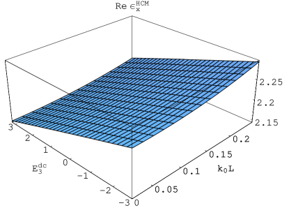
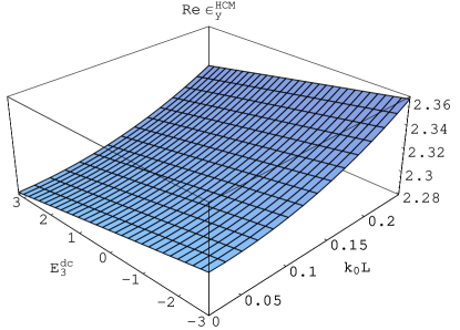
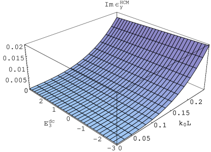
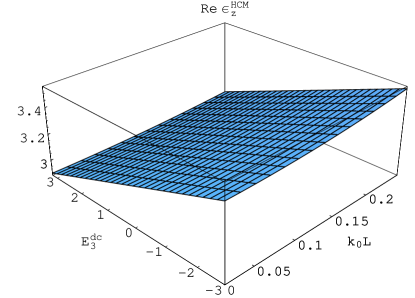
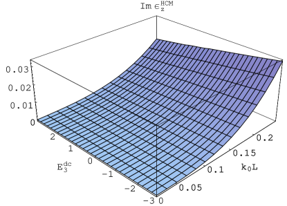
Figure 1: Real (left) and imaginary (right) parts of the HCM’s relative permittivity scalars $\epsilon^{HCM}_{x,y,z}$, as estimated using the SPFT, plotted against $E^{dc}_{3}$ (in V m^-1 $\times 10^{8}$) for $E^{dc}_{1,2}=0$ and $k_{{\scriptscriptstyle 0}}L$. The constituent material $a$ is air and the constituent material $b$ is potassium niobate. The particles of both materials $a$ and $b$ are parallel prolate spheroids, characterized by the shape parameters $\alpha_{1}=\alpha_{2}=1$ and $\alpha_{3}=9$. Calculations were made in the limit $\eta\to 0$.

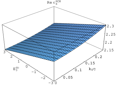
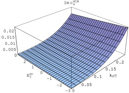
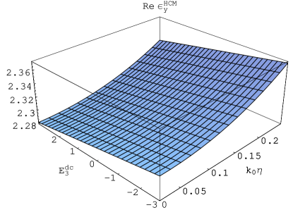
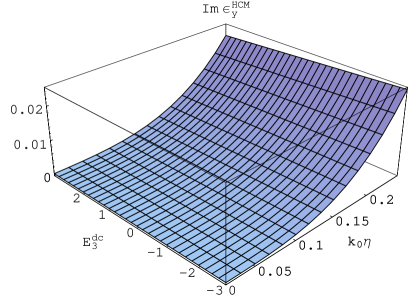
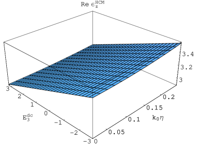
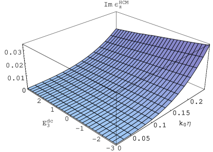
Figure 2: As Figure 1 but with the real (left) and imaginary (right) parts of the HCM permittivity scalars $\epsilon^{HCM}_{x,y,z}$ plotted against $E^{dc}_{3}$ (in V m^-1 $\times 10^{8}$) and $k_{0}\eta$, with correlation length $L=0$.

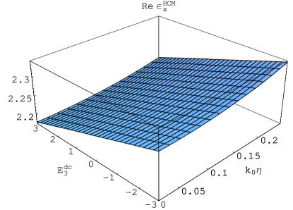
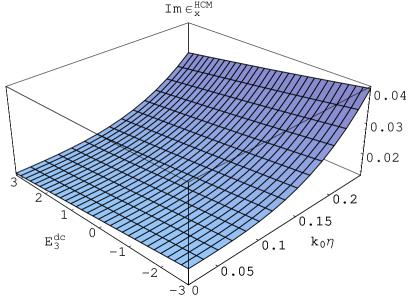
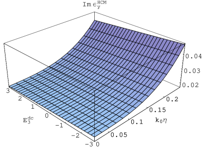
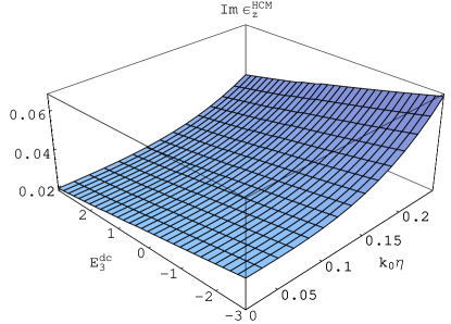
Figure 3: As Figure 1 but with the real (left) and imaginary (right) parts of the HCM permittivity scalars $\epsilon^{HCM}_{x,y,z}$ plotted against $E^{dc}_{3}$ (in V m^-1 $\times 10^{8}$) and $k_{0}\eta$, with $k_{0}L=0.25$.

References

- [1] A. Lakhtakia (ed.), Selected Papers on Linear Optical Composite Materials (SPIE Optical Engineering Press, Bellingham, WA, USA, 1996).
- [2] S.A. Torquato, Random Heterogeneous Materials: Microstructure and Macroscopic Properties (Springer, Heidelberg, Germany, 2002).
- [3] T.G. Mackay, Electromagnetics 25, 461 (2005).
- [4] T. Jaglinski, D. Kochmann, D. Stone, and R.S. Lakes, Science 315, 620 (2007).
- [5] T.G. Mackay and A. Lakhtakia, J. Appl. Phys. 100, 063533 (2006).
- [6] P.S. Neelakanta (ed.), Handbook of Electromagnetic Materials: Monolithic and Composite Versions and their Applications (CRC Press, Boca Raton, FL, USA, 1995).
- [7] R.W. Boyd, Nonlinear Optics (Academic Press, San Diego, CA, USA, 1992).
- [8] K.–H. Hoffmann (ed.), Smart Materials (Springer, Berlin, Germany, 2001).
- [9] A. Lakhtakia, Asian J. Phys. 15, 275 (2006).
- [10] J. Li, M.–H. Lu, L. Feng, X.–P. Liu, and Y.–F. Chen, J. Appl. Phys. 101, 013516 (2007).
- [11] A. Lakhtakia and T.G. Mackay, Proc. R. Soc. A 463, 583 (2007).
- [12] L. Tsang and J.A. Kong, Radio Sci. 16, 303 (1981).
- [13] Z.D. Genchev, Waves Random Media 2, 99 (1992).
- [14] N.P. Zhuck, Phys. Rev. B 50, 15636 (1994).
- [15] T.G. Mackay, Waves Random Media 14, 485 (2004); erratum: Waves Random Complex Media 16, 85 (2006).
- [16] B. Shanker and A. Lakhtakia, J. Phys. D: Appl. Phys. 26, 1746 (1993).
- [17] M.T. Prinkey, A. Lakhtakia, and B. Shanker, Optik 96, 25 (1994).
- [18] L. Tsang, J.A. Kong, and R.W. Newton, IEEE Trans. Antennas Propagat. 30, 292 (1982).
- [19] T.G. Mackay, A. Lakhtakia, and W.S. Weiglhofer, Opt. Commun. 107, 89 (2001).
- [20] B.A. Auld, Acoustic Fields and Waves in Solids (Krieger, Malabar, FL, USA, 1990).
- [21] A. Yariv and P. Yeh, Photonics: Optical Electronics in Modern Communications, 6th ed. (Oxford University Press, New York, NY, USA, 2007).
- [22] A. Lakhtakia, J. Eur. Opt. Soc. – Rapid Pubs. 1, 06006 (2006).
- [23] B. Michel, Int. J. Appl. Electromagn. Mech. 8, 219 (1997).
- [24] M. Zgonik, R. Schlesser, I. Biaggio, E. Volt, J. Tscherry, and P. Günter, J. Appl. Phys. 74, 1287 (1993).