We introduce a dynamical description based on a probability density $\phi(\sigma,x,y,t)$ of the vorticity $\sigma$ in two-dimensional viscous flows such that the average vorticity evolves according to the Navier-Stokes equations. A time-dependent mixing index is defined and the class of probability densities that maximizes this index is studied. The time dependence of the Lagrange multipliers can be chosen in such a way that the masses $m(\sigma,t):=\int\!dxdy\,\phi(\sigma,x,y,t)$ associated with each vorticity value $\sigma$ are conserved. When the masses $m(\sigma,t)$ are conserved then 1) the mixing index satisfies an H-theorem and 2) the mixing index is the time-dependent analogue of the entropy employed in the statistical mechanical theory of inviscid 2D flows [Miller, Weichman & Cross, Phys. Rev. A 45 (1992); Robert & Sommeria, Phys. Rev. Lett. 69, 2776 (1992)]. Within this framework we also show how to reconstruct the probability density of the quasi-stationary coherent structures from the experimentally determined vorticity-stream function relations and we provide a connection between this probability density and an appropriate initial distribution.

1 Introduction

When studying the dynamics of two-dimensional fluid motion characterized by a vorticity field $\omega(x,y,t)$ it can be useful to turn to a statistical description with probability distributions $\phi(\sigma,x,y,t)$ for the microscopic vorticity $\sigma$ such the average value of $\sigma$ over these distributions is equal to $\omega(x,y,t).$ In particular, this has been done in the description of the quasi-stationary states (QSS), i.e., the coherent structures which are often reached in (numerical) experiments after a fast mixing process has taken place[29, 11, 18, 14, 25]. At high Reynolds’ numbers, the vorticity fields $\omega_{S}(x,y)$ of these QSS’s satisfy $\omega-\psi$ relations to a good approximation, i.e., $\omega_{S}(x,y)\simeq\Omega(\psi(x,y))$ where $\psi(x,y)$ is the corresponding stream-function. In other words, the QSS’s are approximate stationary solutions of the Euler equation.

More specifically, in the early 1990’s Miller[16] and Robert[21, 22] together with their coworkers[17, 24, 23]presented a statistical mechanical theory of steady flows in inviscid, two-dimensional fluids, an approach that can be traced back to Linden-Bell’s work of 1967 [13]. Some outstanding aspects of this non-dissipative system are: 1) an infinite number of conserved quantities, the masses associated with each microscopic-vorticity value $\sigma,$ 2) non-uniform steady states or coherent structures, 3) negative-temperature states (already predicted by Onsager’s work on point vortices [19] ). Theoretical predictions were compared with numerical simulations and with experimental measurements in quasi-two dimensional fluids, e.g., in [15, 14, 3, 25, 4]. However, under standard laboratory conditions fluids are viscous. Similarly, numerical simulations require the introduction of a non-vanishing (hyper)viscosity in order to avoid some numerical instabilities and other artifacts. A non-vanishing viscosity can lead to noticeable effects, like the breakdown of the conservation laws, even at high Reynolds’ numbers, i.e., when the viscosity “is small”. This is true especially when studying long-time processes like the generation of the coherent structures. In spite of the dissipative nature of the flows studied, in many cases, it was found that the agreement between the theoretical predictions based on the Miller, Robert and Sommeria (MRS) inviscid theory and (numerical) experiments was better than expected.

The main purpose of the present paper is to better understand these issues in a more dynamical setting. We start by reviewing the MRS theory in Section 2. In Section 3 we consider viscous flows and propose a family of model evolution equations for the vorticity distribution $\phi(\sigma,x,y,t).$ In Sections 4–6 we discuss a class of time-dependent distributions that maximize a mixing index under certain constraints. In particular, in Section 5 it is shown that the time-dependent Lagrange multipliers appearing in these distributions can be chosen in such a way that the masses associated with each microscopic-vorticity value $\sigma$ are conserved. When these masses are conserved, the mixing index is the time-dependent analogue of the entropy functional used by MRS and it satisfies an H-theorem, as it is shown in Appendix A. The distribution $\widetilde{\phi}_{S}(\sigma,\psi(x,y))$ associated with a given QSS can be obtained, at least in principle, by addressing the reconstruction problem, i.e., the question of how to extract its defining parameters from the QSS’s $\omega-\psi$ relation. This is discussed in Section 7. In doing so we provide a natural framework for a time-dependent statistical theory connecting an appropriate initial distribution to the QSS distribution associated with the experimental $\omega-\psi$ relation and evolving in agreement with the Navier-Stokes equation. The relation of the present work with the MRS theory and with the yardsticks’ conditions of reference [6] is discussed in Section 9.

2 The Miller-Robert-Sommeria (MRS) Theory

2.1 Review

The pillars on which the statistical mechanical approach[17, 24] stands are the conserved quantities of the non-dissipative Euler equations. These quantities are: 1) the total energy $E_{o}:=2^{-1}\int_{A}\!dx\,dy\,v_{o}^{2}$ where $\overrightarrow{v}_{o}(x,y)$ is the initial velocity field and $A$ is the area occupied by the fluid and 2) the area density, denoted by $g(\sigma)\,d\sigma,$ occupied by fluid with vorticity values between $\sigma$ and $\sigma+d\sigma,$ which is

$$g(\sigma):=\int_{A}\!dx\,dy\,\phi(\sigma,x,y),$$

where $\phi(\sigma,x,y)\geq 0$ is the probability density of finding a microscopic vorticity value $\sigma$ at position $(x,y),$ with

$$\int\!d\sigma\,\phi(\sigma,x,y)=1,\;\mathrm{for}\;\mathrm{all}\;(x,y).$$ (1)

For the sake of simplicity, we will ignore other conserved quantities which may be present due to some symmetries of the domain $A$, like the linear momentum and/or the angular momentum. Averages taken over this distribution will be indicated by $\left\langle\cdots\right\rangle,$ i.e.,

$$\left\langle f(\sigma,x,y)\right\rangle:=\int\!d\sigma\,f(\sigma,x,y)\phi(\sigma,x,y).$$ (2)

The macroscopic vorticity $\omega(x,y)$ is then

$$\omega(x,y)=\left\langle\sigma\right\rangle.$$

It is assumed that the initial area density, denoted by $g_{o}(\sigma),$ is given by

$$g_{o}(\sigma):=\int_{A}\!dx\,dy\,\delta(\sigma-\omega_{o}(x,y)),$$ (3)

where $\omega_{o}(x,y)=\nabla\times\overrightarrow{v_{o}}$ is the initial macroscopic vorticity field.
As usual, one derives the probability distribution for observing, on a microscopic level, a vorticity value $\sigma$ by maximizing the entropy $S$ under the constraints defined by the conserved quantities. The entropy used by Miller, Robert and Sommeria (MRS) is

$$S:=-A^{-1}\int_{A}\!dx\,dy\,\int\!d\sigma\,\phi(\sigma,x,y)\ln\phi(\sigma,x,y),$$ (4)

The probability distribution $\phi_{S}(\sigma,x,y)$ that one obtains by maximizing the entropy $S$ is

$$\phi_{S}(\sigma,x,y) :=Z^{-1}\exp\left[-\beta\sigma\psi(x,y)+\mu(\sigma)\right],$$ (5)

$$\mathrm{with\;}Z(\psi(x,y)) :=\int\!d\sigma\,\exp\left[-\beta\sigma\psi(x,y)+\mu(\sigma)\right],$$

where $\psi(x,y)$ is the stream function, i.e., $-\Delta\psi(x,y)=\omega_{S}(x,y),$ with $\omega_{S}(x,y)$ the macroscopic vorticity field in the most probable state, i.e.,

$$\omega_{S}(x,y)=\int\!d\sigma\,\sigma\phi_{S}(\sigma,x,y).$$

We have then the $\omega$–$\psi$ relation

$$\omega_{S}(x,y) =\Omega(\psi(x,y)),$$

$$\mathrm{with}\ \ \ \ \Omega(\psi) :=\int\!d\sigma\,\sigma\widetilde{\phi}_{S}(\sigma,\psi),$$

$$\mathrm{where}\ \ \ \ \widetilde{\phi}_{S}(\sigma,\psi(x,y)) :=\phi_{S}(\sigma,x,y),$$

which, in an experimental context, is often called the scatter-plot. This is a mean-field approximation, valid for this system [17], see also eq. (7) below. In eq. (5), $\beta$ and $\mu(\sigma)$ are Lagrange multipliers such that the QSS energy $E_{S}$

$$E_{S}=\frac{1}{2}\int_{A}\!dx\,dy\,\omega_{S}(x,y)\psi(x,y)$$

and the QSS microscopic-vorticity area distribution $g_{S}(\sigma),$

$$g_{S}(\sigma):=\int_{A}\!dx\,dy\,\phi_{S}(\sigma,x,y),$$ (6)

have the same values as in the initial vorticity field, i.e., $E_{S}=E_{o}$ and $g_{S}(\sigma)=g_{o}(\sigma).$ The system of equations is closed by

$$\omega_{S}(x,y) =-\Delta\psi,$$ (7)

$$\mathrm{i.e.},\;\ \ \ \Omega(\psi) =-\Delta\psi.$$ (8)

which embodies the mean-field approximation.

Since by construction $g_{S}(\sigma)=g_{o}(\sigma),$ the assumption expressed by Eq. (3) implies that $M_{n}$ the microscopic vorticity moments in the quasi-stationary state,

$$M_{n}:=\int\!d\sigma\,\sigma^{n}g_{S}(\sigma),$$ (9)

equal the macroscopic vorticity moments in the initial state,

$$\int\!d\sigma\,\sigma^{n}g_{o}(\sigma)=\int_{A}\!dx\,dy\,\omega_{o}^{n}(x,y),$$

confer equation (3).

2.2 The initial state

As we have seen, in its standard formulation, the MRS theory introduces an asymmetry in the microscopic characterization of the initial state and that of the final quasi-stationary state. Namely, it is assumed that the initial state is an “unmixed state” for which the microscopic and macroscopic description coincide. This allows to determine $g_{o}(\sigma)$ the microscopic vorticity distribution of the initial state from the macroscopic vorticity field $\omega_{o}(x,y),$ confer eq. (3). By contrast, the microscopic vorticity-area density of the most probable state, $g_{S}(\sigma),$ is given by $\int\!dx\,dy\,\phi_{S}(\sigma,x,y),$ confer eq. (6). In most cases, $G_{S}(\sigma),$ the macroscopic vorticity density of the most probable state,

$$G_{S}(\sigma):=\int_{A}\!dx\,dy\,\delta(\sigma-\omega_{S}(x,y)),$$ (10)

is different from the microscopic vorticity-area density of the most probable state, i.e., $G_{S}(\sigma)\neq g_{S}(\sigma).$ For example, for non-vanishing viscosity the even moments of $G_{S}(\sigma)$ denoted by $\Gamma_{2n},$ i.e.,

$$\Gamma_{2n}:=\int_{A}\!dx\,dy\,\omega_{S}^{2n}(x,y),$$

are smaller than those of $g_{S}(\sigma)$ since in the MRS approach one assumes that $g_{S}(\sigma)=g_{o}(\sigma),$ confer (25) below. This difference between the moments of the macroscopic and those of the microscopic vorticity has led to confusion and to discussions in the literature related to the interpretation of the MRS theory[12, 5].
According to the MRS theory the microscopic-vorticity moments $M_{n}$ of the QSS, confer Equation (9), equal the microscopic-vorticity moments of the $\delta$-type initial distribution defined in (3). In Subsection III B of an earlier paper[6] we have expressed this infinite set of equalities in terms of the $\omega-\psi$ relation and the initial macroscopic vorticity field $\omega_{o}(x,y).$ In order to assess the validity of the MRS approach, we introduced then a yardstick associated with each moment $M_{n},$ see further the discussion in Section 9.

3 Microscopic Viscous Models

From here onwards we deal with time dependent probability densities, i.e., $\phi(\sigma,x,y,t)d\sigma$ is the probability of finding at time $t$ a microscopic vorticity value in the range $(\sigma,\sigma+d\sigma)$ at a position $(x,y)$ which is non-negative and normalized

$$\int\!d\sigma\,\phi(\sigma,x,y,t)=1.$$ (11)

The macroscopic vorticity field is

$$\omega(x,y,t)=\left\langle\sigma\right\rangle,$$ (12)

where the notation introduced in (2) has been extended to the time-dependent case. In the inviscid case, the time evolution of $\phi(\sigma,x,y,t)$ can be taken to be

$$\frac{\partial\phi(\sigma,x,y,t)}{\partial t}+\vec{v}(x,y,t)\cdot\nabla\phi(\sigma,x,y,t)=0,$$ (13)

where the macroscopic, incompressible velocity field $\vec{v}(x,y,t)$ satisfies appropriate boundary conditions and is related to the macroscopic vorticity $\omega(x,y,t)$ by

$$\nabla\times\vec{v}=\omega\widetilde{z},$$ (14)

with $\widetilde{z}$ a unit vector perpendicular to the $(x,y)$-plane. Consequently, the advective term in equation (13) is quadratic in $\phi$ and different values of $\sigma$ are coupled by this term.

In this Section we introduce some model evolution equations for the probability density $\phi(\sigma,x,y,t).$ We demand that these microscopic models be compatible with the macroscopic Navier-Stokes equations. The general form of these models is

$$\frac{\partial\phi(\sigma,x,y,t)}{\partial t}+\vec{v}(x,y,t)\cdot\nabla\phi(\sigma,x,y,t)=\nu O(\sigma,x,y,t),$$ (15)

with $\nu$ the fluid viscosity and $O$ as yet undefined but constrained by 1) the conservation of the total probabilty $\int\!d\sigma\,\phi(\sigma,x,y,t),$ therefore,

$$\int\!d\sigma\,O=0,$$ (16)

and by 2) the macroscopic Navier-Stokes equation should follow from the microscopic model, therefore,

$$\int\!d\sigma\,\sigma O=\Delta\omega(x,y,t),$$ (17)

so that, multiplying both sides of equation (15) by $\sigma,$ integrating them over $\sigma$ and making use of (12) and (17), one gets the Navier-Stokes equation

$$\frac{\partial\omega(x,y,t)}{\partial t}+\vec{v}(x,y,t)\cdot\nabla\omega(x,y,t)=\nu\Delta\omega(x,y,t).$$ (18)

For future convenience, let us introduce

$$O=:\Delta\phi(\sigma,x,y,t)+\overline{O}\phi,$$

with

$$\left\langle\overline{O}\right\rangle =0,$$ (19a)

$$\mathrm{and}\ \ \left\langle\sigma\overline{O}\right\rangle =0,$$

so that the constraints (16) and (17) are satisfied.

It is convenient to introduce the “masses” $m(\sigma,t)$ associated with each value $\sigma$ of the microscopic vorticity,

$$m(\sigma,t):=\int\!dx\,dy\,\phi(\sigma,x,y,t).$$ (20)

In the inviscid case, incompressibility and the fact that the vorticity is just advected by the velocity field, allow for a complete association between a vorticity value $\sigma$ and the area that is occupied by such value. In this case one talks of ‘conservation of the area occupied by a vorticity value’. In fact, in the inviscid case, $\nu=0,$ equation (15) has a solution $\phi(\sigma,x,y,t)=\delta(\sigma-\omega(x,y,t))$ so that the above-defined $m(\sigma,t)$ is indeed the area occupied by the vorticity field with value $\sigma.$ As soon as we introduce a diffusion process, as it is implied by equation (15) with $\nu\neq 0,$ such an identification becomes problematic if not impossible. It is for this reason that we call $m(\sigma,t)$ a “mass” and, by doing so, we stress the obvious analogy with an advection-diffusion process of an infinite number of “chemical species”, one species for each value $\sigma.$

The time derivative of these masses is

$$\frac{\partial m(\sigma,t)}{\partial t}=\nu\int\!dx\,dy\,\overline{O}\phi(\sigma,x,y,t).$$ (21)

In order to derive these time-evolution equations (21) it was assumed that there is no leakage of $\phi(\sigma,x,y,t)$ through the boundary, i.e., that the total flux of $\phi(\sigma,x,y,t)$ through the boundary vanishes,

$$\oint ds\,\vec{n}\cdot\left[\vec{v}(x,y,t)\phi(\sigma,x,y,t)-\nu\vec{\nabla}\phi(\sigma,x,y,t)\right]=0,$$

where the path of the integral is taken over the boundary and $\vec{n}$ is the normal unit vector. These conditions, as well as other boundary conditions that will be used in the sequel, are satisfied, e.g., in the case of periodic boundary conditions as well as by probability fields whose support stays away from the boundary at all times. In the case of impenetrable boundary conditions one has that, on the boundary, $\,\vec{n}\cdot\vec{v}\equiv 0,$ so that the last condition reduces to

$$\oint ds\,\vec{n}\cdot\vec{\nabla}\phi(\sigma,x,y,t)=0.$$ (22)

On a macroscopic level this implies, e.g., that

$$\oint ds\,\vec{n}\cdot\vec{\nabla}\omega(x,y,t)=0$$

and the conservation of the total circulation $\int\!dx\,dy\,\omega(x,y,t).$

The simplest model satisfying the above requirements is the one with $\overline{O}\equiv 0,$ i.e.,

$$\frac{\partial\phi(\sigma,x,y,t)}{\partial t}+\vec{v}(x,y,t)\cdot\nabla\phi(\sigma,x,y,t)=\nu\Delta\phi(\sigma,x,y,t),$$ (23)

with the incompressible velocity field related to the vorticity as in eq. (14). In spite of its simplicity, this model is very instructive because, while it dissipates energy, it has an infinite number of conserved quantities. Indeed, the masses are conserved,

$$\frac{\partial m(\sigma,t)}{\partial t}=0,$$ (24)

confer (21).

One of the consequences of the conservation laws (24) is that all the microscopic-vorticity moments $M_{n}(t):=\int\!d\sigma\,\sigma^{n}m(\sigma,t)$ are constants of the motion, i.e.,

$$\frac{dM_{n}}{dt}=0.$$

In the sequel we shall assume that the conservation of all the microscopic moments $M_{n}$ implies in turn that the masses $m(\sigma,t)$ are conserved. This is the case if certain technical conditions are satisfied, see e.g., [26].
On the other hand, all even moments of the macroscopic vorticity, call them $\Gamma_{2n}(t),$ i.e., all the quantities

$$\Gamma_{2n}(t):=\int\!dx\,dy\,\omega^{2n}(x,y,t),$$

in particular the macroscopic enstrophy $\int\!dx\,dy\,\omega^{2}(x,y,t),$ are dissipated,

$$\frac{d\Gamma_{2n}}{dt}=-\nu 2n(2n-1)\int\!dx\,dy\,\omega^{2(n-1)}\left|\nabla\omega\right|^{2}\leq 0,$$ (25)

as it is implied by the Navier-Stokes equation (18). Also the energy $E=1/2\int\,dxdy\,v^{2}$ is dissipated

$$\frac{dE}{dt}=\nu\int\!dx\,dy\,\vec{v}\cdot\Delta\vec{v}=-\nu\int\!dx\,dy\left[\,\left(\frac{\partial^{2}\psi}{\partial x^{2}}\right)^{2}+\left(\frac{\partial^{2}\psi}{\partial y^{2}}\right)^{2}+2\left(\frac{\partial^{2}\psi}{\partial x\partial y}\right)^{2}\right]\leq 0,$$

where $\psi(x,y,t)$ is the stream-function associated with $\vec{v}(x,y,t)$ and appropriate boundary conditions, e.g., periodic boundary conditions, have been assumed. Under these boundary conditions, one also has,

$$E =\frac{1}{2}\int\!dx\,dy\,\omega\psi,$$

$$\mathrm{and}\ \ \ \frac{dE}{dt} =-\nu\int\!dx\,dy\,\omega^{2}.$$

Notice that the microscopic energy and the macroscopic one coincide,

$$-\frac{1}{2}\int_{A}\!dx\,dy\,\int\!d\sigma\,\int_{A}\!dx^{\prime}\,dy^{\prime}\,\int\!d\sigma^{\prime}\,\sigma\phi(\sigma,x,y,t)K(x,y,x^{\prime},y^{\prime})\sigma^{\prime}\phi(\sigma^{\prime},x^{\prime},y^{\prime},t)=$$

$$-\frac{1}{2}\int_{A}\!dx\,dy\,\int_{A}\!dx^{\prime}\,dy^{\prime}\,\omega(x,y,t)K(x,y,x^{\prime},y^{\prime})\omega(x^{\prime},y^{\prime},t)$$

In this last expression, $K(x,y,x^{\prime},y^{\prime})$ is the Green function solving

$$\Delta K(x,y,x^{\prime},y^{\prime})=\delta(x-x^{\prime})\delta(y-y^{\prime}),$$

and the appropriate boundary conditions.

In conclusion: The viscous Navier-Stokes equation (18) does not exclude the possibility of an infinite number of conserved quantities $m(\sigma,t)$ as defined in equation (20).

In the following Sections we will consider more generic models with $\overline{O}\neq 0$ that conserve the masses $m(\sigma,t).$

4 Chaotic mixing

Considering once more the models defined by equations (23) and (15), we notice that they are advection-diffusion equations for a non-passive scalar $\phi$ with the viscosity $\nu$ playing the role of a diffusion coefficient. This type of equations has been studied extensively, see e.g. [20] and the references therein. It is well-known that a time-dependent velocity field $\vec{v}(x,y,t)$ usually leads to chaotic trajectories, i.e., to the explosive growth of small-scale $\phi$-gradients. These small-scale gradients are then rapidly smoothed out by diffusion, the net result being a very large effective diffusion coefficient, large in comparison to the molecular coefficient $\nu.$

Based on these observations we will consider situations such that during a period of time, starting at $t_{0}$ and ending at $T_{S}$ when a quasi-stationary structure (QSS) is formed, a fast mixing process takes place leading to a probability density, denoted by $\phi_{S}\left(\sigma,x,y\right),$ that maximizes the spatial spreading or mixing of the masses $m(\sigma,T_{S})$ and is such that $\omega_{S}(x,y)=\int\!d\sigma\,\sigma\phi_{S}(\sigma,x,y)$ satisfies the experimentally found $\omega-\psi$ relation. More specifically, we will investigate solutions of equation (15) for suitable $\nu O$ on the right-hand side satisfying the following conditions: i) at time $t=T_{S}$ the solution $\phi(\sigma,x,y,t)$ is the above-mentioned maximally mixed $\phi_{S}(\sigma,x,y)$ complying with the experimental $\omega-\psi$ relation and ii) the mixing takes place much faster than the changes in the masses $m(\sigma,t),$ so that $m(\sigma,T_{S})\cong m(\sigma,t_{0}).$ In order to express these ideas in a quantitative form, we need a mathematical definition of the degree of spreading or mixing of a solute’s mass in a domain. As described in Appendix A, the $0$–order degree of mixing $s_{0}(\sigma,t)$ defined as

$$s_{0}(\sigma,t):=-A^{-1}\int\!dx\,dy\,\phi(\sigma,x,y,t)\ln\left[A\phi(\sigma,x,y,t)/m(\sigma,t)\right],$$ (26)

is the right quantity in order to quantify the mixing of the microscopic-vorticity masses $m(\sigma,t).$ Accordingly, the total vorticity mixing at time $t,$ is measured by

$$S_{0}(t):=\int\!d\sigma\,s_{0}(\sigma,t).$$

More explicitly,

$$S_{0}(t)=-A^{-1}\int\!d\sigma\int\!dx\,dy\,\phi(\sigma,x,y,t)\ln\phi(\sigma,x,y,t)+A^{-1}\int\!d\sigma\,m(\sigma,t)\ln\left[A^{-1}m(\sigma,t)\right].$$ (27)

The first term coincides with the MRS entropy (4). If the masses are conserved, i.e., if $m(\sigma,t)=m\left(\sigma,t_{0}\right),$ then the second term is constant in time. This allows us to give a mathematical definition of fast mixing, namely: fast mixing of $m(\sigma,t)$ takes place in a time interval $(t_{0},T_{S})$ if the following inequalities hold,

$$\left|\frac{\partial s_{0}(\sigma,t)}{\partial t}\right|\gg\frac{1}{A}\left|\frac{\partial m(\sigma,t)}{\partial t}\right|,\ \ \mathrm{for}\ \ t_{0}\leq t\leq T_{S}.$$ (28)

Accordingly, the corresponding microscopic vorticity probability density $\phi_{S}(\sigma,x,y)$ maximizes the total degree of mixing $S_{0}(T_{S})=\int\!d\sigma\,s_{0}(\sigma,T_{S})$ under the constraint that the change in the masses $m(\sigma,t)$ during the time interval $[t_{o},T_{S}]$ is very small.

It turns out that, for our purposes, a second constraint is needed. Here we discuss two possible choices of this second constraint. One possible choice of the second constraint consists in using the macroscopic vorticity $\omega(x,y,t),$ i.e., the solution of the Navier-Stokes equation with initial condition $\omega_{o}(x,y)$ as input. This means that one demands,

$$\int\!d\sigma\,\sigma\phi(\sigma,x,y,t)=\omega(x,y,t).$$

Two points should be stressed: 1) since $\omega(x,y,t)$ is a solution of the Navier-Stokes equation (18) this choice of the second constraint is totally compatible with the presence of viscous dissipation and 2) this choice of the second constraint can be imposed at all times $t,$ not only at time $T_{S}$ when the QSS is present. The probability distributions which are obtained by maximizing the total degree of mixing $S_{0}(t)$ under the constraints of given values $m(\sigma,t)$ for the masses (20) and given the vorticity field $\omega(x,y,t),$ are presented in the next Section.

The second possible choice of the constraint stems from physical evidence that, in high Reynolds’ number, two-dimensional flows, the energy is transported from the small to the large scales and, consequently, it is weakly affected by viscous dissipation. More formally,

$$\frac{dS_{0}(t)}{dt}\gg\frac{1}{E}\left|\frac{dE}{dt}\right|,\ \ \mathrm{for}\ \ t_{0}\leq t\leq T_{S},$$ (29)

Therefore, one maximazes $S_{0}$ under the constraints that the masses and the energy at time $T_{S}$ have some given values $m(\sigma,T_{S})$ and $E(T_{S}).$ Introducing the corresponding Lagrange multipliers $\beta$ and $\widetilde{\mu}(\sigma),$ as well as a Lagrange multiplier $\gamma(x,y)$ associated with the normalization constraint (11), the constrained variation of the degree of mixing  $S_{0}$ leads to

$$0 =\beta\sigma\psi(x,y)+\widetilde{\mu}(\sigma)+\gamma(x,y)+\ln\frac{A\phi_{S}(\sigma,x,y)}{m\left(\sigma\right)},$$ (30)

$$\mathrm{i.e.,\ \ \ \ }\;\phi_{S}(\sigma,x,y) =A^{-1}m(\sigma)\exp(-\beta\sigma\psi(x,y)-\widetilde{\mu}(\sigma)-\gamma(x,y)),$$

where $m(\sigma):=m(\sigma,T_{S}).$ Since $A^{-1}m(\sigma)\geq 0,$ we can define $\mu(\sigma):=-\widetilde{\mu}(\sigma)+\ln A^{-1}m(\sigma)$ and implementing the normalization constraint (1), one arrives at the probability density (5) of the inviscid, statistical mechanics approach. The new elements here are the conditions expressed by (28) and (29), i.e., a criterium for the applicability of these equations in the case of viscous flows. Notice, moreover, that in contraposition to the statistical mechanical approach, we do not require that the energy $E(T_{S})$ and the masses $m(\sigma,T_{S})$ at time $T_{S}$ be equal to their initial values; equations (28) and (29) only express that the changes in these quantities are much smaller than the change in total vorticity mixing in the time interval $(t_{0},T_{S}).$ In the presence of viscosity $E(T_{S})\leq E(t_{o}),$ when the equality holds one recovers exactly the MRS expressions.

In closing this Section, it is worthwhile recalling that under the physical conditions leading to the inequality in (29) the changes in energy are usually much smaller than the changes in enstrophy. This fact is at the basis of the so-called selective-decay hypothesis[15], i.e., the conjecture that the QSSs correspond to macroscopic vorticity fields with energy $E(T_{S})$ which minimize the macroscopic enstrophy $\Gamma_{2}(T_{S}).$ See also [4].

5 The time-dependent extremal distributions

In this Section we investigate the time-dependent probability distributions which are obtained by using the macroscopic vorticity $\omega(x,y,t)$ as second constraint. As it will be shown in the following Subsection, the form of these distributions is,

$$\phi^{\ast}(\sigma,x,y,t) =Z^{-1}\exp\left[\mu(\sigma,t)+\chi(x,y,t)\sigma\right],$$ (31)

$$\mathrm{with\;\ \ \ \ }Z :=\int\!d\sigma\,\exp\left[\sigma\chi(x,y,t)+\mu(\sigma,t)\right].$$ (32)

The functions $\chi(x,y,t)$ and $\mu(\sigma,t)$ will be called the “potentials”. In contrast to the situation in the statistical mechanics approach, these potentials can be time-dependent. Evidently, for these distributions one has $\phi^{\ast}(\sigma,x,y,t)=:\widetilde{\phi}(\sigma,\chi(x,y,t),t),$ therefore the $(x,y)-$dependence of $\omega(x,y,t)$ as well as that of all the higher-order local moments $m_{n}(x,y,t):=\left\langle\sigma^{n}\right\rangle$ and the centered local moments $K_{n}(x,y,t):=\left\langle\left(\sigma-\omega\right)^{n}\right\rangle$ is only through $\chi(x,y,t),$ i.e., $K_{n}(x,y,t)=:\widetilde{K}_{n}(\chi(x,y,t),t),$ moreover,

$$\omega(x,y,t) =:\widetilde{\Omega}(\chi(x,y,t),t),$$

$$\mathrm{and}\ \ \widetilde{m}_{n}(\chi,t) :=\frac{\int\!d\sigma\,\sigma^{n}\exp\left[\mu(\sigma,t)+\chi\sigma\right]}{\int\!d\sigma\,\exp\left[\mu(\sigma,t)+\chi\sigma\right]},$$

$$\mathrm{moreover}\ \ \frac{\partial\widetilde{\Omega}}{\partial\chi} =\widetilde{K}_{2}(\chi,t),\ \ \mathrm{and}\ \ \widetilde{K}_{3}(\chi,t):=\frac{\partial\widetilde{K}_{2}(\chi,t)}{\partial\chi}.$$

As it is easily checked, the local moments $\widetilde{m}_{n}(\chi,t)$ satisfy then $\partial\widetilde{m}_{n}/\partial\chi=\widetilde{m}_{n+1}-\widetilde{\Omega}\widetilde{m}_{n},$ i.e., the following recursion relation holds,

$$\widetilde{m}_{n+1}(\chi,t) =\mathcal{L}\circ\widetilde{m}_{n}(\chi,t),$$ (33)

$$\mathrm{with}\ \ \ \ \mathcal{L} :=\frac{\partial\ }{\partial\chi}+\widetilde{\Omega}(\chi,t).$$ (34)

5.1 Maximum mixing

Time-dependent distributions as in Equation (31) are obtained by maximizing $S_{0}(t),$ the total degree of mixing at time $t,$ under the constraints of i) normalization, confer Equation (11), ii) given values $m(\sigma,t)$ for the masses at time $t$ as defined in (20) and iii) given vorticity field $\omega(x,y,t)$ at time $t,$ i.e., the distribution’s first moment (12), $\left\langle\sigma\right\rangle=\omega(x,y,t).$ Indeed, introducing the corresponding time-dependent Lagrange multipliers $\gamma(x,y,t),\ \widetilde{\mu}(\sigma,t)$ and $\chi(x,y,t)$ and denoting the extremal distribution by $\phi_{M}(\sigma,x,y,t),$ one has that the vanishing of the first-order variation reads

$$0=\gamma(x,y,t)+\chi(x,y,t)\sigma+\widetilde{\mu}(\sigma,t)+\ln\frac{A\phi_{M}(\sigma,x,y,t)}{m(\sigma,t)},$$

from which, in analogy with the derivation of the statistical mechanical formulas in Section 4, one obtains that $\phi_{M}(\sigma,x,y,t)$ has precisely the form of $\phi^{\ast}(\sigma,x,y,t)$ in (31), i.e., $\phi_{M}(\sigma,x,y,t)=\phi^{\ast}(\sigma,x,y,t)$ with $\mu(\sigma,t):=-\widetilde{\mu}(\sigma,t)+\ln A^{-1}m(\sigma,t).$ The potential functions $\chi(x,y,t)$ and $\mu(\sigma,t)$ should be determined from the two following constraints

$$\omega(x,y,t) =Z^{-1}\int\!d\sigma\,\sigma\exp\left[\sigma\chi(x,y,t)+\mu(\sigma,t)\right],$$ (35)

$$\mathrm{and\;\ \ \ }m(\sigma,t) =\int\!dx\,dy\,Z^{-1}\exp\left[\sigma\chi(x,y,t)+\mu(\sigma,t)\right],$$

where the vorticity field $\omega(x,y,t)$ is not a stationary solution of the Euler equations but a time-dependent solution of the Navier-Stokes equations. The main differences with the maximizer $\phi_{S}(\sigma,x,y)$ of the previous Section are that these distributions $\phi_{M}(\sigma,x,y,t)$ are time-dependent and that now there is no energy constraint, therefore, the Lagrange multiplier $\chi(x,y,t)$ is not a linear function of the stream-function $\psi(x,y,t).$ Up till now, the time dependence of $\mu(\sigma,t)$ has been arbitrary, in the next Subsection this time dependence will be determined such that the masses $m(\sigma,t)$ are conserved.

5.2 The time-dependence of $\mu(\sigma,t)$ and the conservation of the total moments

Assume that at all times the probability density has the form given in (31) which is a time dependent probability density such that $S_{0}(t)$ attains its maximum value compatible with $\left\langle\sigma\right\rangle=\omega(x,y,t)$ and given $m(\sigma,t).$ Inserting these expressions in the Navier-Stokes equation (18) and making use of simple algebraic equalities like,

$$\frac{\partial\phi(\sigma,x,y,t)}{\partial t}=\left[\left(\sigma-\omega\right)\frac{\partial\chi}{\partial t}+\frac{\partial\mu(\sigma,t)}{\partial t}-\left\langle\frac{\partial\mu(\sigma,t)}{\partial t}\right\rangle\right]\phi,$$ (36)

and

$$\frac{\partial\omega}{\partial t} =\widetilde{K}_{2}(\chi,t)\frac{\partial\chi}{\partial t}+\left\langle\left(\sigma-\omega\right)\frac{\partial\mu(\sigma,t)}{\partial t}\right\rangle,$$

$$\nabla\phi =\left(\sigma-\omega\right)\phi\nabla\chi,\;\;\nabla\omega=\widetilde{K}_{2}(\chi,t)\nabla\chi,$$

$$\nabla\widetilde{K}_{2} =\widetilde{K}_{3}(\chi,t)\nabla\chi,$$

with $K_{n}:=\left\langle\left(\sigma-\omega\right)^{n}\right\rangle,$ leads to the following relationship between $\partial\chi/\partial t$ and $\partial\mu/\partial t,$

$$\frac{\partial\chi}{\partial t}+\vec{v}\cdot\nabla\chi-\nu\Delta\chi=\nu\frac{K_{3}}{K_{2}}\left|\nabla\chi\right|^{2}-\frac{1}{K_{2}}\left\langle\left(\sigma-\omega\right)\frac{\partial\mu(\sigma,t)}{\partial t}\right\rangle,$$ (37)

Using this expression in order to eliminate $\partial\chi/\partial t$ from (36), one finally arrives at Equation (15) with $\overline{O}(\sigma,x,y,t)$ expressed in terms of $\chi(x,y,t)$ and of $\partial\mu/\partial t.$ Namely, one obtains that

$$\overline{O}(\sigma,x,y,t) =\nu^{-1}\left(\frac{\partial\mu}{\partial t}-\left\langle\frac{\partial\mu}{\partial t}\right\rangle\right)-\nu^{-1}\frac{\left(\sigma-\omega\right)}{K_{2}}\left\langle\left(\sigma-\omega\right)\frac{\partial\mu}{\partial t}\right\rangle+$$ (38)

$$+\left[K_{2}+\frac{K_{3}}{K_{2}}\left(\sigma-\omega\right)-\left(\sigma-\omega\right)^{2}\right]\left|\nabla\chi\right|^{2},$$ (39)

As one can check, this expression satisfies $\left\langle\overline{O}\right\rangle=0$ and $\left\langle\sigma\overline{O}\right\rangle=0$ independently of the specific form of $\partial\mu/\partial t.$ In other words, the $(x,y)$-dependent constraints (11) and (12) hold at all times and for all possible time-dependences of $\mu(\sigma,t).$

From (38) it follows that the simplest viscous model of the type given in Equation (31), with an identically vanishing $\overline{O}(\sigma,x,y,t),$ can only be realized under very special, and rather trivial, conditions. Indeed, since $\overline{O}(\sigma,x,y,t)\equiv 0$ has to hold for any value of $\sigma,$ equation (38) implies that $\partial\mu/\partial t$ must be quadratic in $\sigma$ and that $\left|\nabla\chi\right|^{2}$ may be time-dependent but must be $(x,y)$-independent. Therefore, the simplest viscous model with an extremal distribution as given in (31), $\overline{O}(\sigma,x,y,t)\equiv 0$ and satisfying equation (38) can hold only if $\chi(x,y,t),$ and $\omega(x,y,t)\,$are linear functions of the space coordinates.

For general $\mu(\sigma,t)$ there is no conservation of the masses $m(\sigma,t).$ However, choosing a suitable time-dependence of $\mu(\sigma,t)$ such that

$$\int\!dxdy\,\phi\overline{O}=0,$$ (40)

ensures the conservation of the masses, i.e., $m(\sigma,t)=m(\sigma,t_{o})$ at all times $t,$ confer equation (21). Using equation (38) the last equality is seen to imply that,

$$\int\left[\frac{\partial\mu(\sigma,t)}{\partial t}-\left\langle\frac{\partial\mu(\sigma,t)}{\partial t}\right\rangle-\frac{(\sigma-\omega)}{K_{2}}\left\langle(\sigma-\omega)\frac{\partial\mu(\sigma,t)}{\partial t}\right\rangle\right]\phi(\sigma,x,y,t)\,dxdy =$$ (41)

$$-\nu\int\left[K_{2}+\frac{K_{3}}{K_{2}}\left(\sigma-\omega\right)-\left(\sigma-\omega\right)^{2}\right]\left|\nabla\chi\right|^{2}\phi(\sigma,x,y,t)\,dxdy =$$

This equation is a complicated integro-differential equation for the time-dependence of $\mu(\sigma,t),$ however, using a Taylor expansion $\mu(\sigma,t)=\sum_{k}\mu_{k}(t)\sigma^{k},$ we can derive an infinite set of linear differential equations for the $d\mu_{k}/dt.$ In fact, multiply equation (38) by $\sigma^{n}\phi(\sigma,x,y,t),$ integrate it over $\sigma$ and get then that:

$$\nu\left\langle\sigma^{n}\overline{O}\right\rangle=-\nu\left|\nabla\chi\right|^{2}h_{n2}+{\displaystyle\sum\limits_{k=2}^{\infty}}h_{nk}\frac{d\mu_{k}}{dt}$$

with

$$h_{nk}(x,y,t):=m_{k+n}-m_{k}m_{n}-\frac{\left(m_{n+1}-\omega m_{n}\right)\left(m_{k+1}-\omega m_{k}\right)}{K_{2}},$$

where $m_{n}$ are the local moments $m_{n}(x,y,t):=\left\langle\sigma^{n}\right\rangle.$ The conservation of the moments $M_{n}=\int\!dxdy\,m_{n}(x,y,t)$ requires then that $\int\!dxdy\,\int\!d\sigma\,\sigma^{n}\phi\overline{O}=0$ and hence that,

$${\displaystyle\sum\limits_{k=2}^{\infty}}\frac{d\mu_{k}}{dt}\int\!dxdy\,h_{nk}=\nu\int\!dxdy\,h_{n2}\left|\nabla\chi\right|^{2},\ \ \ n=2,3,....$$ (42)

From this infinite set of equations, linear in $\overset{}{d\mu_{2}}/dt,\overset{}{d\mu_{3}}/dt,....$, the $d\mu_{k}/dt$ can be solved, in principle. We have then a viscous model with an infinite number of conservation laws. Such a viscous model becomes physically more relevant by making it compatible with a quasi-stationary distribution $\widetilde{\phi}_{S}(\sigma,\psi(x,y))$ as given by Equation (5) with associated $\Omega(\psi)$ relation at time $T_{S},$ i.e., at time $T_{S}$ we can associate with $\widetilde{\phi}_{S}(\sigma,\psi(x,y))$ a distribution function as in Equation (31) which is a solution of the time-evolution Equations (15) and (38), with suitable initial conditions such that $\phi^{\ast}(\sigma,x,y,T_{S})=\widetilde{\phi}(\sigma,\chi(x,y,T_{S}),T_{S})=\widetilde{\phi}_{S}(\sigma,\psi(x,y))$ with $\chi(x,y,T_{S})=-\beta\psi(x,y)$ and with $\mu(\sigma,T_{S})=\mu(\sigma).$ The question of reconstructing the distribution function $\widetilde{\phi}_{S}(\sigma,\psi(x,y))$ from the experimental $\omega-\psi$ relation will be addressed in Section 7.

In concluding we want to remark that, as it is shown in Appendix A, an H-theorem holds for the extremal distributions $\phi^{\ast}(\sigma,x,y,t)$ in the case of conserved masses $m(\sigma,t)$ treated in this paper. More precisely, it is for these distributions with conserved masses that one can prove that $dS_{0}(t)/dt\geq 0.$ Such an H-theorem does not hold for the other measures of mixing $S_{r}$ with $r\neq 0$ which are defined and discussed in Appendix A. Therefore, this result fixes the $0$–degree of mixing $S_{0}$ defined in (26)-(27) as the appropiate measure of mixing.

6 Fast-mixing condition

In this paper we are mainly concerned with dynamical models such that $\partial m(\sigma,t)/\partial t\equiv 0,$ as treated in the previous Subsection. In such a case, the inequalities in (28) will always be satisfied and assuming that the probability distribution $\phi$ is of the extremal form given in Equation (31), we can make use of equation (67) in order to write inequality (29) of the fast mixing condition as,

$$\frac{1}{A}\int\!dx\,dy\,\left\langle\left|\nabla\ln\phi\right|^{2}\right\rangle\gg\frac{1}{E}\int\!dx\,dy\,\omega^{2}.$$ (43)

Two observations are in place: the viscosity drops out from the final expression and the r.h.s. is totally determined by the macroscopic vorticity field $\omega(x,y,t).$

Although the energy-related fast-mixing condition (29) does not play a role in obtaining the time-dependent distributions $\phi_{M}(\sigma,x,y,t)=\phi^{\ast}(\sigma,x,y,t),$ it is still an interesting issue to determine to which extent this fast-mixing condition is actually satisfied or not by the $\phi^{\ast}(\sigma,x,y,t)$ distributions or more general $\phi(\sigma,x,y,t)$ satisfying equations (15)-(17). In fact, for high Reynolds’ number one expects that after a time-interval of fast mixing one arrives at a well-mixed probability distribution with $E(T_{S})\lesssim E(t_{o}).$ In order to investigate this in more detail we will 1) derive a lower bound to $\left\langle\left|\nabla\ln\phi\right|^{2}\right\rangle$ and 2) we will investigate the extrema of the l.h.s. of equation (43) taking into account the constraints (11) and (12). As it will be seen, the special distributions defined in equation (31) play a mayor role in both questions.

6.1 Lower bound on $\left\langle\left|\nabla\ln\phi\right|^{2}\right\rangle$

In order to find a lower bound for $\left\langle\left|\nabla\ln\phi\right|^{2}\right\rangle$ in terms of $\left|\nabla\omega\right|^{2}$ we begin by noting that $\nabla\omega=\left\langle\sigma\nabla\ln\phi\right\rangle$ can also be written as $\nabla\omega=\left\langle\left(\sigma-\omega\right)\nabla\ln\phi\right\rangle$ because $\left\langle\nabla\ln\phi\right\rangle=0.$ Applying then the Cauchy-Schwartz inequality to $\left|\nabla\omega\right|^{2}=\left|\left\langle\left(\sigma-\omega\right)\nabla\ln\phi\right\rangle\right|^{2}$ leads to the desired lower bound,

$$\left|\nabla\omega\right|^{2} \leq\left\langle\left(\sigma-\omega\right)^{2}\right\rangle\left\langle\left|\nabla\ln\phi\right|^{2}\right\rangle=K_{2}\left\langle\left|\nabla\ln\phi\right|^{2}\right\rangle,$$ (44)

$$\mathrm{i.e.,}\ \ \ \ \frac{\left|\nabla\omega\right|^{2}}{K_{2}} \leq\left\langle\left|\nabla\ln\phi\right|^{2}\right\rangle,$$

where $K_{2}$ is the centered second moment $K_{2}(x,y,t):=\int\!d\sigma\,\left(\sigma-\omega(x,y,t)\right)^{2}\phi(\sigma,x,y,t).$

The lower bound on $\left\langle\left|\nabla\ln\phi\right|^{2}\right\rangle$ that we have just found means that the fast-mixing condition (43) holds whenever

$$\frac{1}{A}\int\!dx\,dy\,\frac{\left|\nabla\omega\right|^{2}}{K_{2}}\gg\frac{1}{E}\int\!dx\,dy\,\omega^{2},$$

irrespectively of all the higher-order moments with $n>2.$ Recall that $\int\!dx\,dy\,\left|\nabla\omega\right|^{2}$ is directly related to the dissipation of the macroscopic enstrophy $\Gamma_{2},$ confer equation (25) with $n=1$.

It is rather straightforward to determine the family of vorticity distributions, let us call them $\phi_{LB}(\sigma,x,y,t),$ that reach the lower bound in (44), i.e., that satisfy $\left\langle\left|\nabla\ln\phi_{LB}\right|^{2}\right\rangle=K_{2}^{-1}\left|\nabla\omega\right|^{2}.$ In Appendix B it is proved that

$$\phi_{LB}(\sigma,x,y,t)=\phi^{\ast}(\sigma,x,y,t),$$

with $\phi^{\ast}(\sigma,x,y,t)$ as given by equation (31). In the present context, the input for the determination of the potential functions $\mu(\sigma,t)$ and $\chi(x,y,t)$ are the first and second $\sigma-$moments,

$$\omega(x,y,t) =\int\!d\sigma\,\sigma\phi_{LB}(\sigma,x,y,t),$$ (45)

$$\mathrm{and}\ \ K_{2}(x,y,t) =\int\!d\sigma\,\left(\sigma-\omega(x,y,t)\right)^{2}\phi_{LB}(\sigma,x,y,t).$$

6.2 Extrema of $\int\!dx\,dy\,\left\langle\left|\nabla\ln\phi\right|^{2}\right\rangle$

In Appendix C , we investigate the extrema of $\int\!dx\,dy\,\left\langle\left|\nabla\ln\phi\right|^{2}\right\rangle$ taking into account the $(x,y)$-dependent constraints (12) and (11). It turns out that in order to obtain sensible solutions it is necessary to constrain also the distribution’s second moment $\left\langle\sigma^{2}\right\rangle.$ We find that all the extremizer distributions, call them $\phi_{ext}(\sigma,x,y,t),$ are local minima of $\int\!dx\,dy\,\left\langle\left|\nabla\ln\phi\right|^{2}\right\rangle$ and have the form $\phi_{ext}(\sigma,x,y,t)=\phi^{\ast}(\sigma,x,y,t),$ with $\phi^{\ast}(\sigma,x,y,t)$ as in equation (31). This is in total agreement with the lower bound $\left\langle\left|\nabla\ln\phi_{LB}\right|^{2}\right\rangle$ found in the previous Subsection, confer Appendix B. In fact, as one can check,

$$\left\langle\left|\nabla\ln\phi_{ext}\right|^{2}\right\rangle=\frac{\left|\nabla\omega\right|^{2}}{K_{2}},$$

i.e., these extremal distributions $\phi_{ext}$ reach the lower bound (44). In the present case, the potential functions $\mu(\sigma,t)$ and $\chi(x,y,t)$ should be determined from the input functions $\omega(x,y,t)$ and $K_{2}(x,y,t),$ just as in equations (45).

Summing up the results of the two last Subsections: 1) all distributions $\phi(\sigma,x,y,t)$ with first moment $\omega(x,y,t)$ and second moment $m_{2}(x,y,t)=\omega^{2}(x,y,t)+K_{2}(x,y,t),$ satisfy $\left\langle\left|\nabla\ln\phi\right|^{2}\right\rangle\geq\left\langle\left|\nabla\ln\phi_{LB}\right|^{2}\right\rangle=K_{2}^{-1}\left|\nabla\omega\right|^{2}$ ,
2) the lowest possible value of $\left\langle\left|\nabla\ln\phi\right|^{2}\right\rangle$ is achieved for $\phi_{LB}(\sigma,x,y,t)=\phi_{ext}(\sigma,x,y,t)=\phi^{\ast}(\sigma,x,y,t),$ with $\phi^{\ast}(\sigma,x,y,t)$ as in equation (31) and
 3) if $\int\!dx\,dy\,\left(\left|\nabla\omega\right|^{2}/K_{2}\right)\gg(A/E)\int\!dx\,dy\,\omega^{2},$ then the fast-mixing condition (43) holds implying that the energy changes in the time interval $[t_{o},T_{S}]$ are small.

7 Reconstructing $\mu(\sigma)$ from experimental data

Suppose that in an experiment one is given an initial vorticity field with its corresponding energy $E_{o}$ and that one finds, from a time $T_{S}$ onwards, a quasi-stationary vorticity field

$$\omega_{S}(x,y) =\Omega(\psi(x,y)),$$

$$\mathrm{with}\ \ \ \ \psi_{\min} \leq\psi(x,y)\leq\psi_{\max},$$

with a monotonic $\Omega(\psi)$ and an energy $E_{S}\leq E_{o}.$ As we show below this experimental data can be used in order to determine the $\mu(\sigma)$ potential occuring in the quasi-stationary distribution $\widetilde{\phi}_{S}(\sigma,\psi).$ Once the distribution $\widetilde{\phi}_{S}(\sigma,\psi)$ has been reconstructed from the experimental data we can then associate with it a time-dependent distribution function $\phi^{\ast}(\sigma,x,y,t)$ as given by equation (31) which is a solution of the time-evolution Equation (15) with suitable initial conditions and such that at time $t=T_{S}$ one has$\ \phi^{\ast}(\sigma,x,y,T_{S})=\widetilde{\phi}_{M}(\sigma,\chi(x,y,T_{S}),T_{S})=\widetilde{\phi}_{S}(\sigma,\psi(x,y))$ with $\chi=-\beta\psi$ and with $\mu(\sigma,T_{S})=\mu(\sigma).$ Here $\beta$ can be defined such that $M_{2}(T_{S}),$ the second microscopic-vorticity moment of the QSS at time $T_{S},$ is equal to the enstrophy $\Gamma_{2}^{0}$ of the initial vorticity field $\omega(x,y,t_{o}).$ More explicitly, the condition $M_{2}(T_{S})=M_{2}(t_{0})=\Gamma_{2}^{0}$ leads, also in the viscous case, to

$$\beta=-\frac{\int_{A}\!dx\,dy\,\left(d\Omega/d\psi\right)}{\Gamma_{2}^{0}-\Gamma_{2}^{S}},$$ (46)

see further the discussion in Section 9.

The time-dependence of $\mu(\sigma,t)$ is chosen as in Subsection 55.2, i.e., such that all masses $m(\sigma,t)$ are constant in time.

In order to determine the $\mu(\sigma)$ potential from the experimental $\Omega(\psi)$, we notice that any monotonic function, like $\widetilde{\Omega}(\chi),$ can be expressed as

$$\widetilde{\Omega}(\chi) =\frac{d\ }{d\chi}\ln Z(\chi),$$

$$\mathrm{where}\ \ Z(\chi) =\int_{-\infty}^{\infty}\!d\sigma\,\exp\left[\mu(\sigma)+\chi\sigma\right],$$

for some appropriate function $\mu(\sigma).$ From the above formula and demanding that $\chi=-\beta\psi,$ it follows that it is possible to express $Z(\chi)$ in terms of $\Omega(\psi)$,

$$Z(\chi)=\left.\exp\left[-\beta\int_{\psi_{\min}}^{\psi}d\psi^{\prime}\,\Omega(\psi^{\prime})\right]\right|_{\psi=-\chi/\beta},$$

where $\beta$ is determined from the experimental $\Omega(\psi)$ relation using equation (46). In order to illustrate this procedure, we now treat a number of cases in which we can obtain $\mu(\sigma)$ from $\Omega(\psi)$ either analytically or approximately.

7.1 Linear $\omega-\psi$ relation

The case of a linear $\omega-\psi$ scatter plot, i.e.,

$$\Omega_{l}(\psi) =\alpha_{1}\psi,$$

$$\mathrm{or}\ \ \widetilde{\Omega}_{l}(\chi) =-\alpha_{1}\chi/\beta,$$

can be treated rather straightforwardly. In this case one gets,

$$Z_{l}(\chi)=\exp\left[-\frac{\alpha_{1}}{2\beta}\left(\chi^{2}-\chi_{\min}^{2}\right)\right],$$

with $\chi_{\min}^{2}:=-\beta\psi_{\min}.$ As one can check, taking $\mu_{l}(\sigma)$ such that

$$\exp\mu_{l}(\sigma):=\frac{1}{\sqrt{2\pi}}\sqrt{\left|\frac{\beta}{\alpha_{1}}\right|}\exp\left[\frac{\alpha_{1}}{2\beta}\chi_{\min}^{2}\right]\exp\left[\frac{\beta}{2\alpha_{1}}\sigma^{2}\right],$$

with $\alpha_{1}/\beta<0,$ leads to the desired $Z_{l}(\chi),$

$$\int_{-\infty}^{\infty}\!d\sigma\,\exp\left[\mu_{l}(\sigma)+\chi\sigma\right]=\exp\left[\frac{\alpha_{1}}{2\beta}\chi_{\min}^{2}\right]\exp\left[-\frac{\alpha_{1}}{2\beta}\chi^{2}\right]=Z_{l}(\chi).$$

Since

$$\alpha_{1}/\beta <0,\ \ \ \mathrm{and}$$

$$E_{S} =\int_{A}\!dx\,dy\,\omega_{S}\psi_{S}=\frac{1}{\alpha_{1}}\int_{A}\!dx\,dy\,\omega_{S}^{2}>0,$$

it follows that $\alpha_{1}$ is positive and $\beta$ is negative. The corresponding probability density is then

$$\phi_{S}(\sigma,x,y)=\frac{1}{\sqrt{2\pi}}\sqrt{\left|\frac{\beta}{\alpha_{1}}\right|}\exp\left[\frac{\beta}{2\alpha_{1}}\left(\sigma-\alpha_{1}\psi(x,y)\right)^{2}\right],$$

i.e., a Gaussian centered on $\alpha_{1}\psi$ with a width $\sqrt{\alpha_{1}/\left|\beta\right|}$ which has the form of (5) with $\mu(\sigma)=\mu_{2}\sigma^{2}$ and $\mu_{2}=\beta/\left(2\alpha_{1}\right).$ In the present case the expression (46) for $\beta$ reads,

$$\beta=-\frac{\alpha_{1}A}{\Gamma_{2}(0)-\Gamma_{2}(T_{S})},$$ (47)

where $\Gamma_{2}(t)$ is the enstrophy $\int dxdy\,\omega^{2}(x,y,t).$

7.2 General nonlinear $\omega-\psi$ relation

In the more general nonlinear case we first notice that

$$\int_{-\infty}^{\infty}\!d\sigma\,\frac{d\mu(\sigma)}{d\sigma}\exp\left[\mu(\sigma)+\chi\sigma\right]=-\chi Z(\chi)+\left.\exp\left[\mu(\sigma)+\chi\sigma\right]\right|_{-\infty}^{+\infty}.$$

The boundary terms vanish, so that, using the notation of equation (2), one has

$$\left\langle\frac{d\mu(\sigma)}{d\sigma}\right\rangle=-\chi(x,y).$$ (48)

Introducing into this equality the Taylor expansion of $\mu(\sigma),$

$$\mu(\sigma)=\sum_{k=2}\mu_{k}\sigma^{k},\ \ \ \ \mathrm{i.e.,}\ \ \ \frac{d\mu(\sigma)}{d\sigma}=\sum_{k=2}k\mu_{k}\sigma^{k-1},$$

where the coefficients $\mu_{k}$ are independent of $\chi$, one gets,

$$\sum_{k=2}k\mu_{k}m_{k-1}(\chi)=-\chi.$$ (49)

Using the recursion operator $\mathcal{L}$ defined by (33), this equation can be rewritten as,

$$\left[\sum_{k=2}k\mu_{k}\mathcal{L}^{k-2}\right]\circ\widetilde{\Omega}=-\chi,$$ (50)

where $\mathcal{L}^{n+1}:=\mathcal{L}^{n}\circ\mathcal{L}$. Equation (50) is a nonlinear differential equation in $\widetilde{\Omega}(\chi)$ but it can be reduced to a linear equation in the partition function $Z(\chi).$ This simplification is achieved by multiplying both sides of equation (50) by the partition function $Z(\chi),$ and noticing that

$$\mathrm{for}\ \ n \geq 1,\ \ Z(\chi)\mathcal{L}^{n}\circ\widetilde{\Omega}=\frac{d^{n}\left(Z(\chi)\widetilde{\Omega}\right)}{d\chi^{n}},$$ (51)

$$\mathrm{and\ \ for\ \ }n =0,\mathrm{\ }\ \ Z(\chi)\widetilde{\Omega}=\frac{dZ}{d\chi}.$$

One realizes then that (50) reduces to the following linear differential equation,

$$\sum_{k=2}k\mu_{k}\frac{d^{k-1}Z}{d\chi^{k-1}}=-\chi Z,$$ (52)

that the partition function $Z(\chi)$ must satisfy. In Subsection 88.3 and in Appendix D we consider some cases in which Equation (52) can be reduced to a finite-order differential equation.

7.3 Slightly nonlinear $\omega-\psi$ relation

It is often experimentally found that the $\omega-\psi$ plots satisfy $\Omega(-\psi)\simeq-\Omega(\psi).$ The odd character of $\Omega(\psi)$ implies that $\mu(-\sigma)=\mu(\sigma),$ i.e.,

$$\mu(\sigma)=\mu_{2}\sigma^{2}+\mu_{4}\sigma^{4}+\mu_{6}\sigma^{6}+\cdots.$$

Moreover, in many cases these plots are nearly linear. More specifically, in the Taylor expansion for $\mu(\sigma)$ and in

$$\widetilde{\Omega}(\chi)=f_{1}\chi+f_{3}\chi^{3}+f_{5}\chi^{5}+....,\ \ \mathrm{for}\ \ \left|\chi\right|\leq\chi_{\max}$$ (53)

one has that in a substantial interval around $\psi=0$ or $\chi=0$,

$$Z(\chi)=C\exp\left[1+\frac{1}{2}f_{1}\chi^{2}+\frac{1}{4}f_{3}\chi^{4}+\frac{1}{6}f_{5}\chi^{6}+....\right],$$ (54)

with

$$\left|f_{n+2}\right|\chi^{2} <\left|f_{n}\right|\ \ \ \mathrm{for}\ \ \ n=1,3,5,....,$$

$$\mathrm{and}\ \ \ \ \mu_{n+2} <\mu_{2}\mu_{n}\ \ \ \mathrm{for}\ \ \ n=2,4,6,....$$

Inserting these powers expansions of $Z(\chi)$ and $\mu(\sigma)$ into (52) allows us to express the $\left\{\mu_{n}\right\}$ in terms of the $\left\{f_{n}\right\},$ i.e., it allows us to determine the probability density $\exp\mu(\sigma)$ from the experimentally known scatter-plot $\widetilde{\Omega}(\chi).$ For example, retaining terms up to $f_{5}$ and $f_{3}^{2}$ in the Taylor expansion of  Equation (52) one gets that

$$\mu_{2} =-\frac{1}{2}f_{1}^{-1}-\frac{3}{2}f_{3}f_{1}^{-3}+\frac{15}{2}f_{5}f_{1}^{-4}-12f_{3}^{2}f_{1}^{-5},$$

$$\mu_{4} =\frac{1}{4}f_{3}f_{1}^{-4}-\frac{5}{2}f_{5}f_{1}^{-5}+\frac{21}{4}f_{3}^{2}f_{1}^{-6},$$

$$\mu_{6} =\frac{1}{6}f_{5}f_{1}^{-6}-\frac{1}{2}f_{3}^{2}f_{1}^{-7},$$

$$\mu_{8} =\mu_{10}=......=0.$$

8 Conservation of a finite number of total moments

As we have seen in Subsection 55.2 the masses $m(\sigma,t)$ are conserved if the time dependence of $\mu(\sigma,t)$ satisfies equation (41). For the sake of simplicity one can demand less, for example a finite number of total moments $M_{n}$ for $2\leq n\leq N$ will be conserved by requiring that $\mu(\sigma,t)=\sum_{i=2}^{N}\mu_{i}(t)\sigma^{i}+\sum_{i=N+1}^{\infty}\mu_{i}\sigma^{i}$ where the $\mu_{i}$ with $i\geq N+1$ are time independent and $d\mu_{2}/dt,\ldots,\ d\mu_{N}/dt$ satisfy equation (42). In this case the derivation of an H-theorem as given in Appendix A does not go through even if one assumes that $\mu_{i}=0,$ for $i\geq N+1,$ and consequently that $\int\!d\sigma dxdy\,\phi\overline{O}\ln\phi A=0$ holds, confer (67). This is so because the $m(\sigma,t)$ are not conserved and instead of equation (67) one has that

$$\frac{dS_{0}(t)}{dt}=\frac{\nu}{A}\int\!d\sigma\int dx\,dy\,\frac{1}{\phi}\left|\nabla\phi\right|^{2}+\frac{1}{A}\int\!d\sigma\frac{\partial m(\sigma,t)}{\partial t}\left(\ln m(\sigma)+1\right).$$

However, considering that fast mixing takes place at times $t<T_{S}$ for which the changes in masses can be assumed to be small, we still may use equation (43) as the fast-mixing condition. In the present case inequality (28) is not satisfied automatically but only in the following weaker version

$$\left|\frac{\partial\ }{\partial t}\int\!d\sigma\,\sigma^{n}s_{0}(\sigma,t)\right|\gg\frac{1}{A}\left|\frac{dM_{n}(t)}{dt}\right|,\ \ \mathrm{for}\ \ n\geq N+1.$$

8.1 Gaussian distributions conserving the second moment

It is instructive to consider the $N=2$ case, i.e.,

$$\frac{\partial\mu(\sigma,t)}{\partial t}=\frac{d\mu_{2}(t)}{dt}\sigma^{2}.$$

Then from (42) one gets that

$$\frac{d\mu_{2}(t)}{dt}=\nu\frac{\int\!dxdy\,\left[K_{2}^{-1}K_{3}^{2}+K_{2}^{2}-K_{4}\right]\left|\nabla\chi\right|^{2}}{\int\!dxdy\,\left[K_{2}^{-1}K_{3}^{2}+K_{2}^{2}-K_{4}\right]}.$$ (55)

If further $\mu_{k}=0$ for $k>2$ and $\mu_{2}<0,$ we have then that $\left\langle\overline{O}\ln\phi\right\rangle=0$ and the corresponding solution is a Gaussian distribution,

$$\phi_{G}(\sigma,x,y,t)=\sqrt{\frac{\left|\mu_{2}(t)\right|}{\pi}}\exp\left[\mu_{2}(t)\left(\sigma+\frac{\chi(x,y,t)}{2\mu_{2}(t)}\right)^{2}\right].$$

In this case we have a linear $\omega-\psi$ relation and since $\left\langle\sigma\right\rangle=\omega(x,y,t),$ it follows that $\chi(x,y,t)=-2\mu_{2}(t)\omega(x,y,t),$ and $K_{2}(x,y,t)=-\left[2\mu_{2}(t)\right]^{-1}.$The centered moments $K_{n}(x,y,t)$ of these Gaussian distributions are independent of $(x,y)$, therefore the differential equation (55) satisfied by $\mu_{2}(t)$ reduces to,

$$\frac{d\mu_{2}}{dt} =\frac{\nu}{A}\int\!dxdy\,\left|\nabla\chi\right|^{2}$$ (56)

$$=\frac{4\nu}{A}\mu_{2}^{2}(t)\int\!dxdy\,\left|\nabla\omega\right|^{2}.$$

The solution is,

$$\mu_{2}(t) =\frac{\mu_{2}(0)}{\left[1-2A^{-1}\mu_{2}(0)\Delta(t)\right]},$$ (57)

$$\mathrm{where}\ \ \Delta(t) :=2\nu\int_{0}^{t}\!ds~{}\int\!dxdy\,\left|\nabla\omega\right|^{2}\geq 0.$$

From equation (25) with $n=1,$ one sees that $\Delta\left(t\right)$ is the accumulated change in macroscopic enstrophy $\Gamma_{2}(t),$ i.e., $\Delta(t)=\left(\Gamma_{2}(0)-\Gamma_{2}(t)\right).$ Since $\Delta\left(t\right)\geq 0$ grows with time and $\mu_{2}(0)<0,$ it follows that$\ \left|\mu_{2}(t)\right|$ decreases, i.e., the width $1/\sqrt{\left|\mu_{2}(t)\right|}$ gets larger as time increases.
If the initial distribution is sufficiently narrow so that $\left|\mu_{2}(0)\right|\gg A\left[2\Delta(\infty)\right]^{-1}$ then equation (57) tells us that there must exist a time $T^{\prime}$ such that for all later times $t>T^{\prime}$

$$\mathrm{for}\ ~{}t>T^{\prime},\ \ \ \mu_{2}(t)\simeq-A\left[2\Delta(t)\right]^{-1},$$

i.e., the inverse width $\mu_{2}(t)$ becomes independent of its initial value $\mu_{2}(0).$ Often $\Delta(\infty)\simeq\Gamma_{2}(0)$ and the width will become independent of its initial value if $\left|\mu_{2}(0)\right|\gg A\left[2\Gamma_{2}(0)\right]^{-1},$ which depends only on the initial conditions. In particular, for the $\delta-$type initial conditions as in (3) one has that

$$\lim_{t\downarrow 0}\mu_{2}(t)=-\infty,$$

and Equation (57) becomes

$$\mu_{2}(t)=-\frac{A}{2\left(\Gamma_{2}(0)-\Gamma_{2}(t)\right)}.$$ (58)

The condition for fast mixing in the present case reads,

$$\frac{2\left|\mu_{2}(0)\right|}{\left[A-2\mu_{2}(0)\Delta(t)\right]}\int\!dxdy\,\left|\nabla\omega\right|^{2}\gg\frac{1}{E}\int\!dxdy\,\omega^{2}.$$

If the initial distribution is sufficiently narrow, i.e., $\left|\mu_{2}(0)\right|\gg\left[\Delta(\infty)\right]^{-1}$ then the condition for fast mixing at $t>T^{\prime}$ becomes,

$$\frac{2\nu}{A}\int\!dxdy\,\left|\nabla\omega\right|^{2}\gg\frac{\Delta(t)}{E(t)}\int\!dxdy\,\omega^{2}.$$

If the initial flow is unstable then $\left|\nabla\omega\right|^{2}$ can become very large; in fact, these gradients will become larger the smaller the viscosity $\nu.$ Accordingly one conjuctures that even in the limit of vanishingly small viscosity one may have that

$$\lim_{\nu\rightarrow 0}\frac{2\nu}{A}\int\!dxdy\,\left|\nabla\omega\right|^{2}>0,$$

see the analysis presented in [10].

The corresponding dynamical picture would be as follows: due to chaotic mixing $\Delta(t)\,$grows very quickly up to a time $T_{S}$ when $\omega(x,y,T_{S})$ becomes, to a good approximation, a function of the corresponding stream-function, i.e., $\omega(x,y,T_{S})\simeq\Omega(\psi(x,y,T_{S})).$ At this moment one has a stationary solution of the inviscid Euler equations, the (weak) time dependence is due to viscous effects. If the $\omega-\psi$ relation is linear then the quasi-stationary state $\phi_{S}\left(\sigma,x,y\right)$ is in total agreement with the Gaussian solutions $\phi_{G}\left(\sigma,x,y,T_{S}\right)$ provided that the initial distribution is sharp enough, i.e., that $\left|\mu_{2}(0)\right|\gg A\left[2\Delta(\infty)\right]^{-1}$ and that $T_{S}>T^{\prime}.$ In fact, from the linear $\omega-\psi$ relation $\omega=\alpha_{1}\psi$ of Section 7A with $\beta$ satisfying (46) it follows that,

$$\alpha_{1}\psi=-\beta^{-1}\alpha_{1}\chi=-A^{-1}\left(\Gamma_{2}(0)-\Gamma_{2}(T_{S})\right)\chi=\left(2\mu_{2}(T_{S})\right)^{-1}\chi.$$

The Gaussian distributions that we have discussed above conserve only the distribtuion’s second moment. Suppose that at a certain instant $T$ we have a Gaussian distribution, i.e., that $\mu(\sigma,T)=\mu_{2}\sigma^{2},$ can this distribution conserve all moments and stay Gaussian at later times $t>T?$ Equation (41) tells us that for this to be true the following identity should hold,

$$\int\left[\frac{d\mu_{2}}{dt}\left[\sigma^{2}-\left\langle\sigma^{2}\right\rangle-2\omega(\sigma-\omega)\right]\right]\phi(\sigma,x,y,t)\,dxdy =$$

$$-\nu\int\left[K_{2}-\left(\sigma-\omega\right)^{2}\right]\left|\nabla\chi\right|^{2}\phi(\sigma,x,y,t)\,dxdy =,$$

or, after some manipulations, that,

$$\frac{d\mu_{2}}{dt}\int\left[\left(\sigma-\omega\right)^{2}-K_{2}\right]\phi(\sigma,x,y,t)\,dxdy =$$

$$\nu\int\left[\left(\sigma-\omega\right)^{2}-K_{2}\right]\left|\nabla\chi\right|^{2}\phi(\sigma,x,y,t)\,dxdy =$$

Therefore $\left|\nabla\chi\right|^{2}$ must be independent of $\left(x,y\right)$ and so must be $\left|\nabla\omega\right|^{2}$ since $\chi=2\mu_{2}\omega.$ This corresponds to the simplest dynamical model, equation (23) with $\overline{O}\equiv 0.$ Therefore, a Gaussian distribution can conserve the masses $m(\sigma,t)$ only in the very special case of a space independent $\left|\nabla\omega\right|^{2}.$ Moreover, the last equation implies that,

$$\frac{d\mu_{2}}{dt} =\nu\left|\nabla\chi\right|^{2}$$

$$=4\nu\mu_{2}^{2}(t)\left|\nabla\omega\right|^{2},$$

in agreement with our previous results, confer Equation (56).

8.2 More general distributions with conserved second moment

Here we study the family of nonlinear $\mu(\sigma,t)$ with only one time-dependent $\sigma$-scale $q(t),$ i.e.,

$$\mu(\sigma,t)=\widetilde{\mu}(q(t)\sigma),$$

and accordingly,

$$\frac{\partial\mu(\sigma,t)}{\partial t} =\widetilde{\mu}^{\prime}\frac{dq}{dt}\sigma$$ (59)

$$=\frac{\sigma}{q}\frac{\partial\mu}{\partial\sigma}\frac{dq}{dt},$$

where $\widetilde{\mu}^{\prime}:=\left.d\widetilde{\mu}(x)/dx\right|_{x=q\sigma}$ and the time-dependence of $q(t)$ will be determined in the following paragraphs such that the second global moment is conserved, i.e., $M_{2}(t)=\int\!dx\,dy\,\left\langle\sigma^{2}\right\rangle=M_{2}(0).$

The recursion operator $\mathcal{L}$ defined in (33) allows us to write

$$\left\langle\sigma\frac{d\mu}{d\sigma}\right\rangle=\mathcal{L}\left\langle\frac{d\mu}{d\sigma}\right\rangle=-\mathcal{L}{\normalsize\chi,}$$

confer Equation (48). After some algebra, it follows from (59) that,

$$\nu\left\langle\Gamma\right\rangle =-\left(1+\chi\widetilde{\Omega}(\chi)\right)\frac{1}{q}\frac{dq}{dt},$$

$$\nu\left\langle\left(\sigma-\omega\right)\Gamma\right\rangle =-\left(\widetilde{\Omega}+\chi\frac{d\widetilde{\Omega}}{d\chi}\right)\frac{1}{q}\frac{dq}{dt},$$

$$\mathrm{and}\ \ \ \nu\left\langle\sigma^{2}\Gamma\right\rangle =-\frac{1}{q}\frac{dq}{dt}\left[\chi\frac{d^{2}\widetilde{\Omega}}{d\chi^{2}}+3\left(1+\chi\Omega\right)\frac{d\widetilde{\Omega}}{d\chi}+3\Omega^{2}+\chi\Omega^{3}\right].$$

Multiplying equation (38) by $\sigma^{2},$ taking the average over the vorticity distribution and using the expressions we just derived one arrives at,

$$\nu\left\langle\sigma^{2}\overline{O}\right\rangle=\nu\left|\nabla\chi\right|^{2}\left[\frac{K_{3}^{2}}{K_{2}}+K_{2}^{2}-K_{4}\right]-\frac{1}{q}\frac{dq}{dt}\left[2K_{2}-\Omega\frac{K_{3}}{K_{2}}\right].$$

The conservation of the second global moment $M_{2}=\int\!dx\,dy\,\left\langle\sigma^{2}\right\rangle$ requires that $\int\!dx\,dy\,\left\langle\sigma^{2}\overline{O}\right\rangle=0,$ it follows then that $M_{2}(t)$ is conserved if,

$$\frac{1}{q}\frac{dq}{dt}=\nu\frac{\int\!dx\,dy\,\left|\nabla\chi\right|^{2}K_{2}^{-1}\left[K_{3}^{2}+K_{2}^{3}-K_{2}K_{4}\right]}{\int\!dx\,dy\,K_{2}^{-1}\left[2K_{2}^{2}-\Omega K_{3}\right]}.$$

In most cases one will have that $\left[K_{3}^{2}+K_{2}^{3}-K_{2}K_{4}\right]<0$ while $\left[2K_{2}^{2}-\Omega K_{3}\right]>0,$ therefore, the inverse width $q^{2}$ will decrease in time, i.e., the width of the distribution will grow in time. If the distribution is Gaussian then $K_{3}=0,$ $K_{4}=3K_{2}^{2}$ , $K_{2}=-\left[2\mu_{2}(t)\right]^{-1}$ and the last expression becomes,

$$\frac{1}{q}\frac{dq}{dt} =-\nu\frac{\int\!dx\,dy\,\left|\nabla\chi\right|^{2}K_{2}^{2}}{\int\!dx\,dy\,K_{2}}$$

$$=-\nu\frac{K_{2}}{A}\int\!dx\,dy\,\left|\nabla\chi\right|^{2}.$$

This is in agreement with the result given in equation (56).

If $d\widetilde{\mu}(x)/dx$ is a nonlinear function of $x$ then it does not follow that $\int\!d\sigma dxdy\,\phi\overline{O}\ln\left(\phi A\right)=0$ and there is no H-theorem, confer Equation (66). Assume now that at time $T_{S}$ there is a nonlinear $\omega$–$\psi$ relation which can be associated with a distribution of type (31) with a $\mu(\sigma,t)$ as in equation (59). We can choose the value of $\beta$ according to (46) so that $\delta_{2}(0)=0.$ In the context of our non-Gaussian distributions with conserved second moment this means that the distribution $\phi(\sigma,x,y,T_{S})=\widetilde{\phi}_{S}(\sigma,\psi(x,y))$ can be obtained from a $\delta$-function like initial distribution.

8.3 Non-Gaussian distributions with conserved second and fourth moments

Let us now consider the special case when in the Taylor expansion of $\mu(\sigma)$ only $\mu_{2}$ and $\mu_{4}$ do not vanish. Then the differential equation (52) satisfied by the corresponding $Z\left(\chi\right)$ reduces to,

$$2\mu_{2}\frac{dZ}{d\chi}+4\mu_{4}\frac{d^{3}Z}{d\chi^{3}}=-\chi Z\ \ \ \mathrm{with}\ \ \mu_{4}<0,$$ (60)

From this equation one determines the asymptotic behaviour of $\widetilde{\Omega}(\chi)=d\ln Z/d\chi$ as

$$\widetilde{\Omega}(\chi)\underset{\chi\rightarrow\infty}{\rightarrow}\frac{4}{3}\left(\frac{\chi}{4\left|\mu_{4}\right|}\right)^{1/3}+\frac{\mu_{2}}{6\left|\mu_{4}\right|}\left(\frac{\chi}{4\left|\mu_{4}\right|}\right)^{-1/3}+O\left(\frac{4\left|\mu_{4}\right|}{\chi}\right).$$ (61)

We see that in this case $\lim\widetilde{\Omega}(\chi)\rightarrow\pm\infty$ for $\chi\rightarrow\pm\infty.$ In fact, from Equation (52) one can prove that $\widetilde{\Omega}(\chi)$ remains finite in the limit $\left|\chi\right|\rightarrow\infty$ iff infinitely many $\mu_{k}$ do not vanish. Using equation (60) one can express the coefficients $\mu_{2}$ and $\mu_{4}$ in terms of the experimentally determined coefficients of $\widetilde{\Omega}(\chi)=f_{1}\chi+f_{3}\chi^{3}+f_{5}\chi^{5}+.....$ Inserting this expression in equation (60), expanding in powers of $\chi$ and equating the coefficients of $\chi^{2}$ and $\chi^{4}$ on both sides of the resulting equality leads to

$$\mu_{2} =-\frac{2f_{1}^{3}+24f_{1}f_{3}+40f_{5}}{4f_{1}^{4}+36f_{1}^{2}f_{3}+80f_{1}f_{5}-24f_{3}^{2}},$$

$$\mu_{4} =\frac{f_{3}}{4f_{1}^{4}+36f_{1}^{2}f_{3}+80f_{1}f_{5}-24f_{3}^{2}}.$$

In the special case $\mu_{2}=0$ the solution of equation (60) with boundary conditions $Z(0)=1,\,Z^{\prime}(0)=0$ and $Z^{\prime\prime}(0)=0$ is the Meijer G-function or hypergeometric function ${}_{0}F_{2}([\frac{1}{2}\,,\,\frac{3}{4}],\chi^{4}/256\left|\mu_{4}\right|).$ The corresponding $\widetilde{\Omega}(\chi)$ is plotted in Fig. 1. As expected for this special case with $\mu_{2}=0$, around $\chi=0$ the function $\widetilde{\Omega}(\chi)$ is not linear but cubic, i.e., $f_{1}=0$.

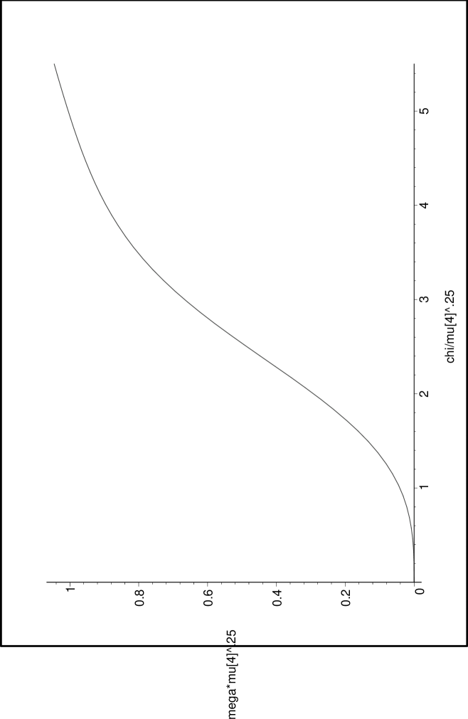
Figure 1: Plot of $\left|\mu_{4}\right|^{1/4}\widetilde{\Omega}$ as a function of $\chi/\left|\mu_{4}\right|^{1/4}$ for the case $\mu(\sigma)=\mu_{4}\sigma^{4}.$

The coefficients $\mu_{2}$ and $\mu_{4}$ in the case of equation (60) can be time-dependent; their time-dependence can be fixed, e.g., by requiring that the second and fourth global moments $M_{2}$ and $M_{4}$ be conserved. Such requirement, i.e., equations (42) with $n=2,4$ and $\mu_{n}=0$ for $n\neq 2,4$ leads to

$$\frac{d\mu_{4}}{dt} =\nu\left[\frac{H_{22}\int dxdy\,\left|\nabla\chi\right|^{2}h_{42}-H_{42}\int dxdy\,\left|\nabla\chi\right|^{2}h_{22}}{h_{22}h_{44}-h_{24}h_{42}}\right],$$

$$\frac{d\mu_{2}}{dt} =\nu\frac{\int dxdy\,\left|\nabla\chi\right|^{2}h_{22}}{H_{22}}-\frac{d\mu_{4}}{dt}\frac{H_{24}}{H_{22}},$$

$$\mathrm{where}\ \ \ \ H_{nm} :=\int dxdy\,h_{nm}$$

and the relation $m_{n}=\sum\limits_{m=0}^{n}\left(\begin{array}[c]{c}n\\ m\end{array}\right)\omega^{m}K_{n-m}$ so that the time-derivatives can be expressed as complicated functions of $K_{2},K_{3},....,K_{8}.$ It is instructive to consider a nearly Gaussian situation in which the $K_{n}$ are replaced by their Gaussian values $K_{2m-1}=0$ and $K_{2m}=(2m-1)!!K_{2}^{m}.$ Then

$$h_{22} =2K_{2}^{2},\ \ h_{42}=12K_{2}^{2}(K_{2}+\omega^{2}),$$

$$h_{44} =24\left(K_{2}^{2}+10K_{2}\omega^{2}+3\omega^{4}\right),$$

$$\frac{d\mu_{4}}{dt} =\frac{\nu}{2}\frac{\int dxdy\,\left|\nabla\omega\right|^{2}\left(\omega^{2}-\Gamma_{2}A^{-1}\right)K_{2}^{-2}}{AK_{2}^{2}+4K_{2}\Gamma_{2}+3(\Gamma_{4}-\Gamma_{2}^{2})},$$

$$\frac{d\mu_{2}}{dt} =\frac{\nu}{AK_{2}^{2}}\int dxdy\,\left|\nabla\omega\right|^{2}-6\left(K_{2}+\Gamma_{2}A^{-1}\right)\frac{d\mu_{4}}{dt}.$$

The expression for $d\mu_{4}/dt$ is governed by the correlation between $\left|\nabla\omega\right|^{2}$ and $\omega^{2}.$ Close to the maxima of $\omega$ the gradient will be very small, analogously the gradient maybe large in the areas where $\omega$ is not close to an extremum. Therefore, it is reasonable to assume that this correlation will be negative, so that $d\mu_{4}/dt\,<0$ while $d\mu_{2}/dt>0.$ This means that, in the context of the models with conserved second and fourth moments, a slightly non-Gaussian initial distribution will evolve into a more strongly non-Gaussian distribution.

9 Discussion and conclusions

In the MRS approach the conservation laws of 2D inviscid flows play a central role. However, the unavoidable viscosity makes these conservation laws invalid; in fact, at high Reynolds’ numbers it is only the energy that is approximately conserved[15]. On the other hand, as we have seen, the conservation of the microscopic-vorticity masses $m(\sigma,t)$ is compatible with a non-vanishing viscosity, it leads to spatial mixing of the masses without destroying or creating them. This is the picture adopted in the present paper.

By working with the family of maximally mixed states studied in Sections 4-6 we reached a mathematical formulation that, as far as the QSS is concerned, shows many parallels with the MRS formulation. In Section 7 we addressed the problem of how to determine the QSS distribution $\phi_{S}(\sigma,x,y)$ from an experimental $\omega-\psi$ relation and $\beta$ given by Equation (46). Identifying this $\phi_{S}(\sigma,x,y)$ with the distribution $\phi(\sigma,x,y,T_{S})=\phi_{M}(\sigma,x,y,T_{S})=\phi_{LB}(\sigma,x,y,T_{S})=\phi^{\ast}(\sigma,x,y,T_{S})$ of Section 5 and using a time-dependent $\mu(\sigma,t)$ satisfying Equations (41)-(42) and such that $\mu(\sigma,T_{S})=\mu(\sigma)$ we have a dynamical model that conserves the masses, i.e. with $m(\sigma,t)=m(\sigma,t_{o}),$ and connects the experimental $\omega-\psi$ relation found at time $T_{S}$ with an initial condition $\phi(\sigma,x,y,t_{o}).$ An extra bonus that follows from this methodology is that an H-theorem holds, moreover, it holds for one measure of spatial mixing, namely for the $S_{0}$ degree of mixing, confer Appendix A. When the masses $m(\sigma,t)$ are conserved, this mixing measure $S_{0}$ coincides with the MRS entropy.

In Subsection III B of an earlier paper[6] we expressed the quantities $\delta_{n}$

$$\delta_{n}:=\int\!d\sigma\int\!dxdy\,\left[\sigma^{n}-\omega_{S}^{n}(x,y)\right]\phi_{S}(\sigma,x,y),$$

in terms of spatial integrals of certain polynomials in $\Omega(\psi)$ and its derivatives $d^{r}\Omega/d\psi^{r}.$ For example, for $n=2,$ one has that

$$\delta_{2}=-\frac{1}{\beta}\int_{A}\!dx\,dy\,\frac{d\Omega}{d\psi}.$$

and the MRS assumption $0=\delta_{2}+\Gamma_{2}^{S}-\Gamma_{2}^{0}$, can be used, as we did in Section 7, in order to determine $\beta$ from the experimentally accessible quantities $\Omega(\psi)$ and the initial and final enstrophies $\Gamma_{2}^{0}$ and $\Gamma_{2}^{S}$ as in Equation (46). From these $\delta_{n}$ one finds the corresponding initial values

$$\delta_{n}^{o}:=\int\!d\sigma\int\!dxdy\,\left[\sigma^{n}-\omega_{o}^{n}(x,y)\right]\phi(\sigma,x,y,t_{o}),$$

because the conservation of the moments $M_{n}$ implies that$\ \delta_{n}^{o}=\delta_{n}+\Gamma_{n}^{S}-\Gamma_{n}^{0},$ where $\Gamma_{n}^{S}:=\int\!dx\,dy\,\omega_{S}^{n}(x,y)$ and $\Gamma_{n}^{0}:=\int\!dx\,dy\,\omega_{o}^{n}(x,y)$ are the macroscopic-vorticity moments in the QSS and in the initial state, repectively. In the MRS approach the initial distribution is assumed to be a $\delta$-function as in Equation (3), consequently, all $\delta_{n}^{o}$ should vanish. This led us in [6] to propose the quantities,

$$\frac{\delta_{n}}{\Gamma_{n}^{0}-\Gamma_{n}^{S}},\ \ n=2,3,....$$ (62)

as yardsticks in order to investigate the validity of the statistical mechanical approach according to which all these quantities should equal 1. Choosing $\beta$ as in (46) the yardstick relation $\delta_{2}/\left(\Gamma_{2}^{0}-\Gamma_{2}^{S}\right)=1$ is automatically satisfied while the remaining yardsticks for $n>2$ are nontrivial checks for the validity of the statistical mechanics approach. When all the yardsticks relations $\delta_{n}/(\Gamma_{n}^{o}-\Gamma_{n})=1$ hold the quasi-stationary state predicted by the MRS approach is in agreement with the experimental $\omega-\psi$ relation, moreover, it is also the solution of equation (15) at time $T_{S}$ with conserved total moments $M_{n}$ and starting from the initial condition $\phi(\sigma,x,y,t_{o})=\delta(\sigma-\omega_{0}(x,y)).$ When not all the yardsticks relations are satisfied then the MRS approach gives an incorrect but approximate prediction of the experimental $\Omega(\psi)$ relation. In such a case it still may be possible to obtain a rather sharp initial distribution, which is determined by the experimental $\Omega(\psi)$ relation, such that the quasi-stationary state is the solution of equation (15) at time $T_{S}$ and with conserved total moments $M_{n}(T_{S})=M_{n}(t_{o}).$

Hence it maybe concluded that our class of dynamical models with non-vanishing viscosity and with conserved masses yields a self-consistent dynamical description containing the MRS approach with $\delta-$type initial conditions in the case that the experimental values of the yardsticks relations are 1 and with different initial conditions in all other cases. In these other cases the predictive power of the statistical mechanics approach, i.e., the prediction of the correct QSS on the basis of a $\delta-$type initial condition, is lost and the reconstruction of the correct initial distribution in the context of the models with conserved masses is a rather difficult if not forbidding problem. In such cases it may be more convenient to give up the conservation of all masses, require that only the second moment $M_{2}$ be conserved and use the Gaussian distributions of Subsection 88.1 if the $\omega-\psi$ relation is linear or the family of $\mu(\sigma,t)$ with only one time-dependent scale $q(t)$ of Subsection 88.2 in the case of a nonlinear $\omega-\psi$ relation.

Appendix A Degrees of mixing

A mass of solute $m$ achieves the highest degree of mixing when it is homogeneously distributed over the area $A,$ i.e., when its concentration is constant and equal to $m/A.$ Let us introduce $\delta(\sigma,x,y,t)$ the spatial distribution of the $\sigma$-species at time $t,$ i.e.,

$$\delta(\sigma,x,y,t) :=\frac{\phi(\sigma,x,y,t)}{m(\sigma,t)}\geq 0,$$

$$\int\!dx\,dy\,\delta(\sigma,x,y,t) =1.$$

In order to determine how well mixed is this $\sigma$-mass one has to determine ‘how close’ is the corresponding $\delta(\sigma,x,y,t)$ to the homogeneous distribution $1/A.$ As it is known[1], given two spatial densities, called them $\delta_{1}(x,y)$ and $\delta_{2}(x,y),$ there is a one-parameter family of non-negative, convex functionals $d_{r}(\delta_{1},\delta_{2})$ satisfying $d_{r}(\delta_{1},\delta_{2})=0\longleftrightarrow\delta_{1}\overset{a.e.}{=}\delta_{2}$ and measuring a sort of distance between them, namely

$$d_{r}(\delta_{1},\delta_{2}):=\left[r(1-r)\right]^{-1}\int\!dx\,dy\,\delta_{1}(x,y)\left[1-\left(\delta_{2}(x,y)/\delta_{1}(x,y)\right)^{r}\right]\geq 0,\;0<r<1,$$

and, by imposing continuity in $r,$

$$d_{0}(\delta_{1},\delta_{2}) :=-\int\!dx\,dy\,\delta_{1}(x,y)\ln\left(\delta_{2}(x,y)/\delta_{1}(x,y)\right),$$

$$d_{1}(\delta_{1},\delta_{2}) :=-\int\!dx\,dy\,\delta_{2}(x,y)\ln\left(\delta_{1}(x,y)/\delta_{2}(x,y)\right).$$

For $r>1$ and for $r<0$, they may diverge. However, since in our case $\delta_{2}(x,y)=1/A\neq 0,$ values $r<0$ would also be possible. The $d_{r}$ are not distances because, e.g., for $r\neq 1/2,$ they are asymmetric in their arguments, i.e., $d_{r}(\delta_{1},\delta_{2})\neq d_{r}(\delta_{2},\delta_{1}).$

Accordingly, we can measure the mixing degree of the $\sigma$-mass by $-d_{r}(\delta(\sigma,x,y,t),1/A).$ Its weighted contribution to the total mixing degree will be denoted by $s_{r}(\sigma,t),$ i.e.,

$$s_{r}(\sigma,t) :=m(\sigma,t)\left[Ar(r-1)\right]^{-1}\int\!dx\,dy\,\delta(\sigma,x,y,t)\left[1-\left(1/A\delta(\sigma,x,y,t)\right)^{r}\right]\leq 0,\;\mathrm{for}\;0<r<1,$$

$$s_{0}(\sigma,t) :=-m(\sigma,t)A^{-1}\int\!dx\,dy\,\delta(\sigma,x,y,t)\ln A\delta(\sigma,x,y,t)$$

$$=-A^{-1}\int\!dx\,dy\,\phi(\sigma,x,y,t)\ln\left[\frac{A\phi(\sigma,x,y,t)}{m(\sigma,t)}\right]\leq 0,$$

$$s_{1}(\sigma,t) :=m(\sigma,t)A^{-1}\int\!dx\,dy\,\ln A\delta(\sigma,x,y,t)\leq 0,$$

the corresponding total $r$-order degree of mixing is then,

$$S_{r}(t) :=\left[Ar(r-1)\right]^{-1}\int\!d\sigma\int\!dx\,dy\,\phi(\sigma,x,y,t)\left[1-\left(m(\sigma,t)/A\phi(\sigma,x,y,t)\right)^{r}\right]\leq 0,\;0<r<1,$$ (63)

$$S_{0}(t) :=-A^{-1}\int\!d\sigma\int\!dx\,dy\,\phi(\sigma,x,y,t)\ln\left[A\phi(\sigma,x,y,t)/m(\sigma,t)\right]\leq 0.$$

Under certain conditions, these degrees of mixing satisfy a kind of H-theorem. In order to see this, let us compute the time derivative of $s_{r}(\sigma,t),$ with $0<r<1,$

$$\frac{\partial s_{r}(\sigma,t)}{\partial t}=\frac{1}{Ar\left(r-1\right)}\int\!dx\,dy\,\left\{\left[1+\frac{\left(r-1\right)m^{r}}{\left(A\phi\right)^{r}}\right]\frac{\partial\phi}{\partial t}-\frac{r}{A}\left(\frac{m}{A\phi}\right)^{(r-1)}\frac{\partial m}{\partial t}\right\},$$

and consider the mass-consevation models with $\partial m/\partial t=0$ so that $\partial s_{r}(\sigma,t)/\partial t$ is totally determined by the first term in the curly brackets and one has that,

$$\frac{\partial s_{r}(\sigma,t)}{\partial t} =\frac{1}{r\left(r-1\right)A}\int\!dx\,dy\,\left\{\left[1+\frac{\left(r-1\right)m^{r}(\sigma)}{\left(A\phi\right)^{r}}\right]\left[-\vec{v}\cdot\nabla\phi+\nu\Delta\phi+\nu\overline{O}\phi\right]\right\}$$ (64)

$$=\frac{\nu}{A}\int\!dx\,dy\,\frac{m^{r}(\sigma)}{\left(A\phi\right)^{r}}\left[\frac{\left|\nabla\phi\right|^{2}}{\phi}+\frac{1}{r}\overline{O}\phi\right]\ \ \mathrm{with}\;0<r<1,$$ (65)

While for $r=0,$

$$\frac{\partial s_{0}(\sigma,t)}{\partial t} =\frac{\nu}{A}\int\!dx\,dy\,\phi\left[\left|\frac{\nabla\phi}{\phi}\right|^{2}+\overline{O}\ln\frac{m(\sigma)}{A\phi}\right]$$ (66)

$$=\frac{\nu}{A}\int\!dx\,dy\,\phi\left[\left|\frac{\nabla\phi}{\phi}\right|^{2}-\overline{O}\ln A\phi\right].$$

In the simplest viscous model with $\overline{O}=0,$ the last formulas lead to a H-theorem for each $\sigma$-value,

$$\frac{\partial s_{r}(\sigma,t)}{\partial t}=\frac{\nu}{A}\int\!dx\,dy\,\frac{m^{r}(\sigma)}{\left(A\phi\right)^{r}}\frac{\left|\nabla\phi\right|^{2}}{\phi}\geq 0,\ \mathrm{with}\;0\leq r\leq 1.$$

In the more general viscous model with $\overline{O}\neq 0$ and conservation of the total moments, i.e., with $\int\!dx\,dy\,\left\langle\sigma^{n}\overline{O}\right\rangle=0,$ one can prove an H-theorem only for the total 0-th order mixing $S_{0}(t).$ This is done by assuming that $\phi$ is of the form given in (31) so that $\ln\phi$ can be expressed as a power series in $\sigma$ in which only the constant and linear terms may depend upon $(x,y),$ i.e., $\ln\phi=\chi(x,y,t)\sigma+\sum_{i=2}\mu_{i}(t)\sigma^{i}-\ln Z(\chi,t).$ In such a case the term containing $\overline{O}$ in (66) vanishes since by construction $\left\langle\overline{O}\right\rangle=\left\langle\sigma\overline{O}\right\rangle=0,$ confer (19), and one gets that

$$\frac{dS_{0}(t)}{dt}=\frac{\nu}{A}\int\!d\sigma\int dx\,dy\,\frac{1}{\phi}\left|\nabla\phi\right|^{2}\geq 0.$$ (67)

It is for this reason that the only mixing measure considered in the body of this paper is the 0-th order $S_{0}(t).$ Non-extensive quantities like $s_{r}(\sigma,t)$ with $r\neq 0$ have been considered as possible generalizations of the Boltzmann entropy, see e.g.[28] and in the context of 2D fluid motion[2] , confer also reference [4] in which some useful comments are given.

Appendix B

In order to determine the family of probability densities $\phi_{LB}(\sigma,x,y,t)$ that reach the lower bound in (44), i.e., $\left\langle\left|\nabla\ln\phi_{LB}\right|^{2}\right\rangle=K_{2}^{-1}\left|\nabla\omega\right|^{2},$ we write

$$\ln\phi=:\sum_{n=0}b_{n}(x,y,t)\sigma^{n},$$

and notice that, due to the normalization condition (11), one has that

$$\exp\left(-b_{0}(x,y,t)\right)=\int\!d\sigma\,\exp\left(\sum_{n=1}b_{n}(x,y,t)\sigma^{n}\right).$$

It follows then that,

$$\nabla b_{0}(x,y,t)=-\sum_{n=1}\left\langle\sigma^{n}\right\rangle\nabla b_{n}(x,y,t),$$

and consequently that

$$\nabla\ln\phi =\sum_{n=1}\left[\sigma^{n}-\left\langle\sigma^{n}\right\rangle\right]\nabla b_{n}(x,y,t),$$

$$\mathrm{and}\ \ \nabla\omega =\sum_{n=1}\left\langle\left(\sigma-\omega\right)\left[\sigma^{n}-\left\langle\sigma^{n}\right\rangle\right]\right\rangle\nabla b_{n}(x,y,t).$$

It is now easy to see that if for $n\geq 2$ one has $\nabla b_{n}=0$ then $\left\langle\left|\nabla\ln\phi\right|^{2}\right\rangle=\left\langle\left(\sigma-\omega\right)^{2}\right\rangle\left|\nabla b_{1}\right|^{2}$ and also $\nabla\omega=\left\langle\left(\sigma-\omega\right)^{2}\right\rangle\nabla b_{1}(x,y,t),$ i.e., $\left|\nabla\omega\right|^{2}=K_{2}^{2}\left|\nabla b_{1}\right|^{2}.$ Therefore, in this special case with $\nabla b_{n}=0$ for $n\geq 2$ the equality $\left|\nabla\omega\right|^{2}=K_{2}\left\langle\left|\nabla\ln\phi\right|^{2}\right\rangle$ holds. We have shown then that $\phi_{LB}(\sigma,x,y,t)$ can be identified with $\phi^{\ast}(\sigma,x,y,t)$ as given in Equation (31) with

$$\chi(x,y,t) :=b_{1}(x,y,t),$$

$$\mathrm{and}\ \ \ \mu(\sigma,t) :=\sum_{n=2}\mu_{n}(t)\sigma^{n},\ \ \ \nabla\mu_{n}=0,$$

and that it attains the lower bound in (44), i.e.,

$$\left\langle\left|\nabla\ln\phi_{LB}\right|^{2}\right\rangle=\frac{\left|\nabla\omega\right|^{2}}{K_{2}}.$$

Appendix C First and second variation of $\int\!dx\,dy\,\left\langle\left|\nabla\ln\phi\right|^{2}\right\rangle$

In this Appendix we investigate the extrema of $\int\!dx\,dy\,\left\langle\left|\nabla\ln\phi\right|^{2}\right\rangle$ when $\phi$ satisfies (11), (12) as well as

$$\int d\sigma\,\sigma^{2}\phi(\sigma,x,y,t)=m_{2}(x,y,t).$$

The quantity we have to vary, let us call it $T(\phi),$ is then

$$T(\phi):=\frac{1}{\phi}\left|\nabla\phi\right|^{2}+\sum_{n=0}^{2}\lambda_{n}(x,y,t)\sigma^{n}\phi,$$

where $\lambda_{n}(x,y,t)$ are the Langrange multipliers corresponding to the local-moments constraints $m_{0}(x,y,t)\equiv 1,\ m_{1}(x,y,t)=\omega(x,y,t)$ and $m_{2}(x,y,t)$. Up to second-order terms in $\delta\phi$ we have

$$T(\phi+\delta\phi)-T(\phi) =2\nabla\cdot\left(\delta\phi\nabla\ln\phi\right)+\delta_{1}T+\delta_{2}T,$$

$$\mathrm{with}\ \ \delta_{1}T :=\left[\frac{1}{\phi^{2}}\left|\nabla\phi\right|^{2}-2\frac{\Delta\phi}{\phi}+\sum_{n=0}^{2}\lambda_{n}(x,y)\sigma^{n}\right]\delta\phi,$$

$$\mathrm{and}\ \ \delta_{2}T :=\frac{1}{\phi}\left[\nabla\delta\phi-\frac{\nabla\phi}{\phi}\delta\phi\right]^{2}.$$

The first term is a total divergence that, upon integration over $(x,y),$ leads to a vanishing boundary term. The extrema are determined by $\delta_{1}T=0$ and since $\delta_{2}T\geq 0$ it follows that all extrema are minima of $\int\!dx\,dy\,\left\langle\left|\nabla\ln\phi\right|^{2}\right\rangle$ under the given constraints. In order to solve $\delta_{1}T=0$ it is convenient to introduce $e(\sigma,x,y,t):=\phi^{1/2}$ and noticing then that

$$\Delta e=\frac{1}{2}\left(\frac{\Delta\phi}{\phi}-\frac{1}{2}\frac{\left|\nabla\phi\right|^{2}}{\phi^{2}}\right)e,$$

one sees that $\delta_{1}T=0$ is equivalent to

$$\Delta e=\frac{1}{4}\left(\sum_{n=0}^{2}\lambda_{n}(x,y)\sigma^{n}\right)e.$$

Let us denote the minimizer of $T(\phi)$ by $\phi_{ext}(\sigma,x,y,t),$ i.e., $\delta_{1}T(\phi_{ext})=0.$ As one can check, this minimizer can be written as

$$\phi_{ext}(\sigma,x,y,t) =\exp\left[\mu(\sigma,t)+b_{0}(x,y,t)+\chi(x,y,t)\sigma\right],$$

$$\mathrm{where}\ \ \exp\left[-b_{0}(x,y,t)\right] :={\displaystyle\int}\!\!d\sigma\,\exp\left[\mu(\sigma,t)+\chi(x,y,t)\sigma\right],$$

which can thus be identified with $\phi^{\ast}(\sigma,x,y,t)$ as given in Equation (31). In this extremal case, the Lagrange multipliers are,

$$\lambda_{0} =\omega^{2}\left|\nabla\chi\right|^{2}-2\omega\Delta\chi-2\nabla\chi\cdot\nabla\omega$$

$$=\left[K_{2}\right]^{-2}\left[\left(\omega^{2}-2K_{2}\right)\left|\nabla\omega\right|^{2}-2K_{2}\omega\left(\Delta\omega-\nabla\omega\cdot\nabla\ln K_{2}\right)\right],$$

$$\lambda_{1} =4\Delta\chi-2\omega\left|\nabla\chi\right|^{2}$$

$$=\left[K_{2}\right]^{-2}\left[2K_{2}\left(\Delta\omega-\nabla\omega\cdot\nabla\ln K_{2}\right)-2\omega\left|\nabla\omega\right|^{2}\right],$$

$$\lambda_{2} =\left|\nabla\chi\right|^{2}=\left[K_{2}\right]^{-2}\left|\nabla\omega\right|^{2},$$

$$\lambda_{n}(x,y,t) =0,\ \ \mathrm{for}\ \ n=3,4,....$$

Appendix D Cases associated with finite-order differental equations

The differential equations (50) and (52) are of infinite order, however, in some cases they reduce to finite–order differential equations in a non-trivial way. For example, when $\mu(\sigma)$ is such that

$$\frac{d\mu}{d\sigma}=-2q^{2}\frac{P_{N}(q\sigma)}{Q_{M}(q\sigma)}\sigma,$$ (68)

where $P_{N}(x)$ and $Q_{M}(x)$ are polynomials in $x$ of order $N$ and $M,$ respectively, $\lim_{x\rightarrow 0}P_{N}(x)=\lim_{x\rightarrow 0}Q_{M}(x)$ and $q$ is a parameter such that $q\sigma$ is dimensionless. Then equation (48) reads

$$2q^{2}\left\langle\frac{P_{N}(q\sigma)}{Q_{M}(q\sigma)}\sigma\right\rangle=\chi,$$

and using the recursion operator $\mathcal{L}$ defined in (33), it follows that

$$2q^{2}P_{N}(q\mathcal{L})\widetilde{\Omega}(\chi)=Q_{M}(q\mathcal{L})\chi.$$

The remarkable disappearance of the $\sigma-$average can be traced back to the special $\chi-$dependence of the extremal distributions, confer equation (33). Making now use of equation (51), the linear differential equation (52) that $Z(\chi)$ must satisfy when (68) holds follows, namely

$$2q^{2}P_{N}(q\frac{d\ }{d\chi})\frac{dZ}{d\chi}=Q_{M}(q\frac{d\ }{d\chi})\left(\chi Z\right).$$ (69)

In Subsection 88.3 a case with $N=2$ and $M=0$ was considered. An example with $P_{N}(x)=1$ is provided by a $\mu(\sigma)$ of the following form,

$$\mu_{d}(\sigma):=\left\{\begin{array}[c]{c}d^{-2}\ln\left[1-d^{2}q^{2}\sigma^{2}\right]\ \ \ \mathrm{for}\ \ \sigma^{2}<\left[dq\right]^{-2},\\ -\infty\ \ \ \ \mathrm{for}\ \ \ \ \sigma^{2}\geq\left[dq\right]^{-2},\end{array}\right.$$

where $d$ is a pure number. For finite $d$ the vorticity distribution has a finite support, $\sigma^{2}<\left[dq\right]^{-2},$ while in the limit $d\rightarrow 0$ it approaches a Gaussian. Since

$$\frac{d\mu_{d}}{d\sigma}=-\frac{2q^{2}\sigma}{1-d^{2}q^{2}\sigma^{2}},$$

the differential equation satisfied by the corresponding partition function $Z_{d}$ is

$$2q^{2}\frac{dZ_{d}}{d\chi} =\left[1-d^{2}q^{2}\frac{d^{2}\ }{d\chi^{2}}\right]\left(\chi Z_{d}\right),$$

$$\mathrm{i.e.,}\ \ \ \frac{d^{2}Z_{d}}{d\chi^{2}}+\frac{2}{\chi}(1+d^{-2})\frac{dZ_{d}}{d\chi}-\frac{Z_{d}}{q^{2}d^{2}} =0.$$

This is a modified Bessel equation of fractional order. The corresponding boundary conditions are $Z_{d}(0)=1$ and $Z_{d}^{\prime}(0)=0$. The solution is:

$$Z_{d}(\chi)=\left(\frac{q}{\chi}\right)^{\alpha}Y_{\alpha}(\frac{\chi}{qd}),$$

where $Y_{\alpha}(\chi/qd)$ is a modified Bessel function of fractional order and $\alpha:=(d^{2}+2)/2d^{2}.$ Indeed, since in the present case $\exp\mu_{d}(\sigma)=\left[1-d^{2}q^{2}\sigma^{2}\right]^{1/d^{2}}$ for $\sigma^{2}<1/\left(q^{2}d^{2}\right)$ and $0$ otherwise, we have that

$$Z_{d}(\chi) =\int_{-1/qd}^{1/qd}\!d\sigma\,\left[1-d^{2}q^{2}\sigma^{2}\right]^{1/d^{2}}\exp\chi\sigma$$

$$=\frac{1}{qd}\int_{-1}^{1}\!ds\,\left[1-s^{2}\right]^{1/d^{2}}\exp\left(\frac{\chi s}{qd}\right)$$

$$\propto\left(\frac{qd}{\chi}\right)^{\alpha}\mathrm{Y}_{\alpha}(\frac{\chi}{qd}),$$

corresponding to the integral representation of the modified Bessel functions. As one can check $\lim_{\chi\rightarrow\infty}\widetilde{\Omega}(\chi)=\left[qd\right]^{-1}$and $\lim_{\chi\rightarrow 0}d\widetilde{\Omega}/d\chi=1/q(3d^{2}+2).$The graph in Fig. 2 shows the corresponding $\widetilde{\Omega}(\chi)$ for the cases $d=1$ and $d=3.$

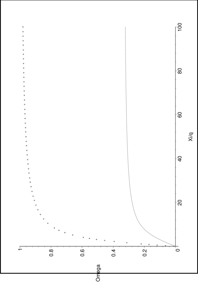
Figure 2: Plot of $q\widetilde{\Omega}$ as a function of $\chi/q$ for $d=1$ (crosses) and $\ d=3$ (full line).

References

- [1] C. Arndt, Information measures, Spinger, Berlin, 2001.
- [2] B. M. Boghosian, “Thermodynamic description of the relaxation of 2D turbulence using Tsallis statistics”, Phys. Rev. E 53, 4754 (1996).
- [3] H. Brands, J. Stulemeyer, R.A. Pasmanter and T.J. Schep, “A mean field prediction of the asymptotic state of decaying 2D turbulence”, Phys. Fluids 9 2815, (1998).
- [4] H. Brands, P.-H. Chavanis, R.A. Pasmanter and J. Sommeria, “Maximum entropy versus minimum enstrophy vortices”, Phys. Fluids 11, 3465 (1999).
- [5] H. Brands, J. Stulemeyer, R.A. Pasmanter and T.J. Schep, Response to “Comment on ‘A mean field prediction of the asymptotic state of decaying 2D turbulence’ ”, Phys. Fluids 10 1238, (1998).
- [6] H.W. Capel and R.A. Pasmanter, “Evolution of the vorticity-area density during the formation of coherent structures in two-dimensional flows”, Phys. Fluids 12, 2514 (2000).
- [7] O. Cardoso, D. Marteau and P. Tabeling, “Quantitative experimental study of the free decay of quasi-two-dimensional turbulence”, Phys. Rev. E 49, 454 (1994)
- [8] P.-H. Chavanis and J. Sommeria, “Classification of robust isolated vortices in two-dimensional turbulence”, J. Fluid Mechanics 356, 259–296 (1998).
- [9] P.-H. Chavanis, “Statistical mechanics of two-dimensional vortices and stellar systems”, in “Dynamics and Thermodynamics of Systems with Long Range Interactions”, T. Dauxois, S. Ruffo, E. Arimondo, M. Wilkens Eds., Lecture Notes in Physics Vol. 602, Springer (2002).
- [10] G. L. Eyink, “Dissipation in turbulent solutions of 2D Euler equations”, Nonlinearity 14, 787 (2001).
- [11] G.J.F. van Heijst and J.B. Flor, “Dipole formations and collisions in a stratified fluid”, Nature 340, 212 (1989)
- [12] W.H. Matthaeus and D. Montgomery, Comment on “A mean field prediction of the asymptotic state of decaying 2D turbulence”, Physics of Fluids 10, 1237 (1998).
- [13] D. Lynden-Bell, “Statistical mechanics of violent relaxation in stellar systems”, Mon. Not. R. Astro. Soc. 136, 101 (1967).
- [14] D. Marteau, O. Cardoso, and P. Tabeling, “Equilibrium states of 2D turbulence: an experimental study”. Phys. Rev. E 51, 5124-5127 (1995).
- [15] W.H. Matthaeus, W. T. Stribling, D. Martinez, S. Oughton and D. Montgomery, “Selective decay and coherent vortices in two-dimensional incompressible turbulence”, Phys. Rev. Letters 66, 2731 (1991) and the references therein.
- [16] J. Miller, “Statistical mechanics of Euler’s equation in two dimensions”, Phys. Rev. Lett. 65, 2137 (1990).
- [17] J. Miller, P.B. Weichman, and M.C. Cross, “Statistical mechanics, Euler’s equation, and Jupiter’s Red Spot”, Phys. Rev. A 45, 2328 (1992).
- [18] D. Montgomery, X. Shan, and W. Matthaeus, “Navier-Stokes relaxation to sinh-Poisson states at finite Reynolds numbers”, Phys. Fluids A 5, 2207 (1993).
- [19] L. Onsager, “Statistical Hydrodynamics”, Nuovo Cimento Suppl. 6, 279-287 (1949).
- [20] J. M. Ottino, “Mixing, chaotic advection and turbulence”, Annual Rev. Fluid Mech. 22, 207 (1990).
- [21] R. Robert, “Etat d’équilibre statistique pour l’écoulement bidimensionnel d’un fluide parfait, C. R. Acad. Sci. Paris 311 (Série I), 575 (1990).
- [22] R. Robert, “Maximum entropy principle for two-dimensional Euler equations”, J. Stat. Phys. 65, 531 (1991).
- [23] R.Robert and J. Sommeria, “Relaxation towards a statistical equilibrium state in two-dimensional perfect fluid dynamics”, Phys. Rev. Lett. 69, 2776 (1992).
- [24] R. Robert and J. Sommeria, “Statistical equilibrium states for two dimensional flows”, J. Fluid Mech. 229, 291 (1991).
- [25] E. Segre and S. Kida, “Late states of incompressible 2D decaying vorticity fields”, Fluid Dyn. Res. 23, 89 (1998).
- [26] J. A. Shohat and J. D. Tamarkin, The problem of moments, Amer. Math. Soc. Math. Surveys, no. 1, 1943.
- [27] J. Sommeria, C. Staquet, and R. Robert, “Final equilibrium state of a two dimensional shear layer”, J. Fluid Mech. 233, 661 (1991).
- [28] C. Tsallis, “Possible generalization of Boltzmann-Gibbs statistics”, J. Stat. Phys. 52, 479 (1988); See also http://tsallis.cat.cbpf.br/biblio.htm.
- [29] J.C. McWilliams, “The emergence of isolated coherent vortices in turbulent flow”, J. Fluid Mech. 146, 21 (1984).