Intramolecular vibrational energy redistribution as state space diffusion: Classical-Quantum correspondence

Abstract

We study the intramolecular vibrational energy redistribution (IVR) dynamics of an effective spectroscopic Hamiltonian describing the four coupled high frequency modes of CDBrClF. The IVR dynamics ensuing from nearly isoenergetic zeroth-order states, an edge (overtone) and an interior (combination) state, is studied from a state space diffusion perspective. A wavelet based time-frequency analysis reveals an inhomogeneous phase space due to the trapping of classical trajectories. Consequently the interior state has a smaller effective IVR dimension as compared to the edge state.

Investigating the dynamics of an initially localized vibrational excitation of a molecule in terms of timescales, final destinations and competing pathways has been of considerable interest to chemical physicists for a number of decadesum91 ; Kel95 ; Ezr98 ; nf96 ; kp00 ; Gru00 ; gw04 . Due to the sustained theoreticalum91 ; Kel95 ; Ezr98 ; gw04 and experimental effortsnf96 ; kp00 ; Gru00 ; gw04 it is only now that a fairly detailed picture of the intramolecular vibrational energy flow is beginning to emerge. Recent studiessw92 ; sw95 ; sww95 ; sww96 suggest that IVR can be described as a diffusion in the zeroth-order quantum number space (also known as the state space) mediated by the anharmonic resonances coupling the zeroth-order states. The state space approachGru00 makes several predictions on the observables associated with IVR. Foremost among them is that an initial zeroth-order bright state $|b\rangle$ diffuses anisotropically on a manifold of dimension $D$ much smaller than $N$ (or $N-1$ with energy constraint). $N$ is the number of vibrational modes in the molecule. As a result the survival probability $P_{b}(t)$ exhibits power law behaviour on intermediate time scales

$$P_{b}(t)=|\langle b|b(t)\rangle|^{2}\sim\sigma_{b}+(1-\sigma_{b})\left[1+\frac{2t}{\tau D}\right]^{-D/2}$$ (1)

with $\sigma_{b}=\sum_{\alpha}|\langle b|\alpha\rangle|^{4}$ being the dilution factor of the zeroth-order state $|b\rangle$ and $|\alpha\rangle$ denoting the eigenstates of the system. Wong and Gruebelewg99 explained the power law behaviour from the state space perspective by providing a perturbative estimate for $D$ as:

$$D\approx D(n)=\frac{\Delta\ln\sum_{i}L_{ib}^{2}}{\Delta\ln n}$$ (2)

with $n=|{\bf n}_{i}-{\bf n}_{b}|$ being the distance, in state space, from the state $|b\rangle$ to other states $|i\rangle$ and the sum is over all states $|i\rangle$ such that $|{\bf n}_{i}-{\bf n}_{b}|\leq n$. The zeroth-order quantum numbers $n_{k}$ are associated with the state $|k\rangle$ and the symbol $\Delta$ indicates a finite difference evaluation of the dimension due to the discrete nature of the state space. In practice one chooses two different distances $n$ in the state space and evaluates eq. 2 and thus $D\approx D(n)$. The quantity

$$N_{loc}(|b\rangle)\equiv\sum_{i}L_{ib}^{2}=\sum_{i}\left[1+\left(\frac{\Delta E^{0}_{ib}}{V_{ib}}\right)^{2}\right]^{-1}$$ (3)

is a measure of the number of states locally coupled to $|b\rangle$. The difference in the zeroth-order energies is denoted by $\Delta E^{0}_{ib}=E^{0}_{i}-E^{0}_{b}$ and $V_{ib}=\langle i|V|b\rangle$. Notice that in the strong coupling limit, $\Delta E^{0}_{ib}\ll V_{ib}$, $L_{ib}\approx 1$ whereas in the opposite limit $L_{ib}\approx 0.$ Thus $D_{v}(n)$ can range between the full state space dimension and zerowg99 . For further discussions on the origin and approximations inherent to eq. 2 we refer the reader to the original referencewg99 . In the context of the present study it is sufficient to note that $D\propto N_{loc}$ which has been confirmed in the earlier workwg99 .

Clearly Eq. 2 explicitly includes the various anharmonic resonances and hence not only the local nature but the directionality of the energy flow is also taken into account. The main point is that the above estimate for $D$, which can be obtained without computing the actual dynamics, is crucially dependent on the nature of the IVR diffusion in the state space. However, to the best of our knowledge, precious little is known about the dynamics associated with the state space diffusion. Our motivation for investigating the IVR dynamics in the state space has to do with the observation that the state space model shares many of the important features found in the classical-quantum correspondence studies of IVRum91 ; Ezr98 ; Kel95 . Classical dynamical studies identify the nonlinear resonance network as the crucial object. On such a network, directionality and the local nature of IVR arises rather naturally mainly due to the reason that molecular phase spaces are mixed regular-chaotic even at fairly high energies. How does the mixed phase space influence the IVR diffusion in the state space? Is there any relation, and hence correlation, between the classical resonance network and the IVR dimension $D$ in the state space? Is it possible that local dynamical traps in the classical phase space can affect the validity of Eq. 2? Answers to these questions can have significant impact on our ability to control IVR and hence reaction dynamics. The issues involved are subtle and this preliminary work attempts to address the questions by studying a specific system.

Although detailed classical-quantum correspondence studies of IVR have been performedum91 ; Kel95 ; Ezr98 ; Kes99 on systems with two degrees of freedom, in order to address the questions one needs to analyze atleast a three degree of freedom case. This is due to the fact that the scaling theory of Schofield and Wolynes posits $D=2$ as the critical scaling i.e., near the IVR thresholdsw92 . Thus for systems with two degrees of freedom the separation of diffusive and critical regimes is not very sharpKes99 . However, studying IVR from the phase space perspective is difficult in systems with three or more degrees of freedom. In this study we use a time-frequency technique proposed by Arevalo and Wigginsaw01 to construct a useful phase space representation of the resonance network for three degrees of freedom. Such an approach, as seen below and in many recent studiessk03 ; bhc05 , is particularly well suited for our purpose. Thus we choose an effective spectroscopic Hamiltonianbhmqs00 describing the energy flow dynamics between the four high frequency modes of CDBrClF. The Hamiltonian $H=H_{0}+V_{res}$ with the anharmonic zeroth-order part

$$H_{0}=\sum_{j}\omega_{j}a_{j}^{\dagger}a_{j}+\sum_{i\leq j}x_{ij}a_{i}^{\dagger}a_{i}a_{j}^{\dagger}a_{j}$$ (4)

has various anharmonic resonances coupling the four normal modes denoted by $s$ (CD-stretch), $f$ (CF-stretch) and $(a,b)$ (CD-bending modes)

$$V_{res} = \sum_{j\leq m}^{a,b,f}\frac{k_{sjm}}{2\sqrt{2}}(a_{s}a_{j}^{\dagger}a_{m}^{\dagger}+a_{s}^{\dagger}a_{j}a_{m})$$ (5)

$$+ \frac{1}{2}\sum_{j<m}^{a,b,f}\gamma_{jm}(a_{j}^{\dagger}a_{j}^{\dagger}a_{m}a_{m}+a_{j}a_{j}a_{m}^{\dagger}a_{m}^{\dagger})$$

The harmonic creation and destruction operators for the j^th mode are denoted by $a_{j}^{\dagger}$ and $a_{j}$ respectively. Note that despite having four coupled modes the system has effectively three degrees of freedom due to the existence of a conserved polyad $N=v_{s}+(v_{f}+v_{a}+v_{b})/2$. In this work we choose $N=5$ for illustrating the main idea. Similar results are seen in other systems and the details will be published later. The values of the various parameters are taken from the fit in referencebhmqs00 (fourth column, Table VIII). The Fermi resonance strengths $k_{sjm}$ are larger then the mean energy level spacings (13.7 cm^-1 $\sim$ 2.5 ps) of $H_{0}$ for $N=5$. Thus this is an example of a strongly coupled system and the multiple Fermi resonances render the classical dynamics irregular. We investigate the IVR dynamics out of two nearly isoenergetic zeroth-order states $|v_{s},v_{f},v_{a},v_{b}\rangle=|5000\rangle,$ and $|3301\rangle$ denoted for convenience as $|1\rangle$ and $|2\rangle$ respectively. The experimentally accessible state $|1\rangle$ has energy $E^{0}_{1}\approx 10571$ cm^-1 whereas the combination state has $E^{0}_{2}\approx 10567$ cm${}^{-1}\approx E^{0}_{1}$. We restrict our study to these two states although there are other close by states within a mean level spacing. In terms of their location in state space the state $|1\rangle$ is an example of an edge state whereas $|2\rangle$ is an example of an interior state.

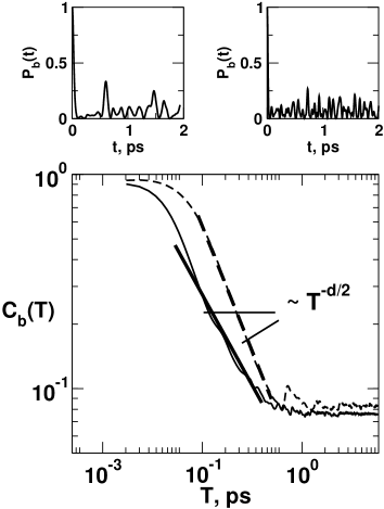
Figure 1: Survival probabilities $P_{b}(t)$ and time-smoothed survival probabilities $C_{b}(T)$ for the two isoenergetic states. The left and right top panels show $P_{b}(t)$ for $|1\rangle$ and $|2\rangle$ respectively. Intermediate time power law behaviour is exhibited by $C_{b}(T)$ in both cases, dashed line (state $|1\rangle$) and solid line (state $|2\rangle$). Note that the $C_{b}(T)$ data is shown for $T=10$ ps indicating small oscillations about the respective dilution factors $\sigma_{b}$.

Given the Hamiltonian and the resonant couplings the number of states coupled locally to $|1\rangle$ and $|2\rangle$ can be estimated as $N_{loc}=1.8$, and $3.0$ respectively. Combined with the fact that $N_{eff}\equiv\sigma_{b}^{-1}\approx 12$ one expects fast IVR from both the states. Since $N_{loc}(|1\rangle)<N_{loc}(|2\rangle)$ the decay is much faster at short times for $|2\rangle$. This is confirmed in Fig. 1 which shows $P_{b}(t)$ for the states. However Fig. 1 also shows the time-smoothed survival probabilitykpg92 ; hs94

$$C_{b}(T)=\frac{1}{T}\int_{0}^{T}dtP_{b}(t)$$ (6)

associated with the states and, importantly, highlights a power law behavior of $C_{b}(T)\sim T^{-d/2}$ at intermediate times - a sign of incomplete IVRwg99 ; gw04 . Note that the persistent recurrences in $P_{b}(t)$ occur for much longer times as evident from the results for $C_{b}(T)$. Earlier workskpg92 ; hs94 , in an apparently different context, have associated the power law behaviour with the multifractality of the eigenstates and the local density of states. The power law exponent or effective IVR dimensionality in the state space are determined to be $d_{1}\sim 1.8$ and $d_{2}\sim 1.3$ which are smaller than the three dimensional state space. Incidentally, a purely exponential decay of $P_{b}(t)$ would imply $C_{b}(T)\sim T^{-1}$ irrespective of the dimensionality of the state space. More surprising observation from Fig. 1 is that the interior state shows faster short time IVR but at longer times, despite $N^{(2)}_{loc}>N^{(1)}_{loc}$, explores an IVR manifold of smaller dimension as compared to the edge state. Infact based on $N_{loc}$ and the strong couplings one would infer the opposite from Eq. 2.

Since $E^{0}_{1}\approx E^{0}_{2}$ the results in Fig. 1 suggest different IVR mechanisms for the two states. This can be established by correlating the intensities $p_{b\alpha}=|\langle b|\alpha\rangle|^{2}$ with the parametric variation of eigenvalues $E_{\alpha}(\tau)$ i.e, the intensity-level velocity correlation functionTom96 ; kct02 :

$$L_{b}(\tau)=\frac{1}{\sigma_{p}\sigma_{v}}\left\langle p_{b\alpha}\frac{\partial E_{\alpha}}{\partial\tau}\right\rangle_{\Delta E}$$ (7)

where $\sigma_{p}$ and $\sigma_{v}$ denote the intensity and level velocity variances respectively. The parameter $\tau$ corresponds to the resonant coupling strengths in eq. 5 and $\Delta E$ is the width of the IVR feature. Recent workkct02 has shown that $L_{b}(\tau)$ can identify the dominant resonances that control the IVR dynamics. In Fig. 2 we show the correlator $L_{b}(\tau)$ for $|1\rangle$ and $|2\rangle$. Random matrix theory (RMT) predictsTom96 $L_{b}(\tau)\sim 0\pm 1/\sqrt{N}$ with $N$ being the number of eigenstates under the IVR feature and hence ergodicity implies a vanishing correlator for any state of choice. It is clear from Fig. 2 that several of the correlators violate the RMT estimate indicating localization. In particular $L_{b}(\tau)$ indicates differing IVR dynamics out of $|1\rangle$ and $|2\rangle$. For instance, $L_{b}(k_{sff})$ for the states differ by about $0.2$ which is greater than the fluctuations allowed by RMT ($\approx 0.11$). Note that the results in Fig. 2 support the local RMT approachlw90 ; lw97 , developed by Logan, Leitner, and Wolynes, which is consistent with the power law decay of $P_{b}(t)$ and thus $d\sim D$ (cf. eq. 2).

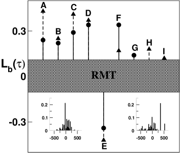
Figure 2: Intensity-level velocity correlator $L_{b}(\tau)$ for $|b\rangle=|1\rangle$ (circles) and $|2\rangle$ (triangles). The random matrix (RMT) estimate is shown by the shaded region. The parameter $\tau$ are taken to be the various resonant strengths and the $sff,saa,sbb,sfa,sfb,sab,aabb,ffaa,$ and $ffbb$ resonances are denoted by A,B,…,I respectively. The averaging is performed over a range $\Delta E=\pm 700cm^{-1}$ corresponding to the width of the IVR feature as seen in the insets (Left inset corresponds to $|1\rangle$ and the right inset to $|2\rangle$).

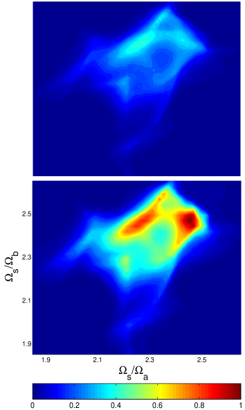
Figure 3: Dynamical Arnol’d web plotted in the frequency ratio space $(\Omega_{s}/\Omega_{a},\Omega_{s}/\Omega_{b})$ for $|1\rangle$ (top) and $|2\rangle$ (bottom). The scale for the axes is identical for both the figures. The data is obtained by propagating $5000$ trajectories with fixed initial actions corresponding to the state of interest and varying angles such that $H({\bf I},{\bm{\theta}})\approx E^{0}_{b}$. The color scale (normalized) indicates the number of times that a region is visited by the trajectories. Total propagation time $T=10$ ps and note that the figures look similar already by about $T=2.5$ ps.

We now show that the observed power law in Fig. 1 and the slower IVR dynamics of the interior state $|2\rangle$ are due to the existence of dynamical traps in the classical phase space. First the classical limit Hamiltonian $H({\bf I},{\bm{\theta}})$ is constructed using the correspondenceKel95 $a_{j}\rightarrow\sqrt{I_{j}}e^{i\theta_{j}}$ with $({\bf I},{\bm{\theta}})$ being the action-angle variables of $H_{0}$. Next, classical trajectories with initial conditions such that $H({\bf I},{\bm{\theta}})\approx E_{b}^{0}$ and actions ${\bf I}$ restricted to the specific state are generated. For every trajectory the dynamical function $z_{k}(t)=\sqrt{2I_{k}(t)}\exp(i\theta_{k}(t))$ with $k=s,f,a,b$ is subjected to the wavelet transformaw01 :

$$W_{g}z_{k}(A,B)=A^{-1/2}\int_{-\infty}^{\infty}z_{k}(t)g^{*}\left(\frac{t-B}{A}\right)dt$$ (8)

with $A>0$ and real $B$. The function $g(t)=(2\pi\sigma^{2})^{-1/2}\exp(2\pi i\lambda t-t^{2}/\sigma^{2})$ is taken to be the simple Morlet-Grossman waveletaw01 with $\lambda=1$ and $\sigma=2$. Eq. 8 yields the frequency content of $z_{k}(t)$ over a time window around $t=B$. In this work we obtain the local frequency associated with $z_{k}(t)$ by determining the scale ($A$, inversely proportional to frequency) which maximizes the modulus of the wavelet transform i.e., $\Omega_{k}(t=B)={\rm max}_{A}|W_{g}z_{k}(A,B)|$. This gives the nonlinear frequencies ${\bm{\Omega}}(t)$ and the dynamics at $E=E^{0}_{b}$ is followed in the frequency ratio spacemde87 $(\Omega_{s}/\Omega_{a},\Omega_{s}/\Omega_{b})$. The frequency ratio space is divided into cells and the number of times that a cell is visited for all the trajectories gives the density plot. We further normalize the highest density to one for convenience. Two points should be noted at this stage. First, such a density plot is providing a glimpse of the energy shell and is reflecting the full dynamics including the important resonances. Thus we are mapping out parts of the Arnol’d web i.e., the resonance network that is actually utilized by the system. Secondly, we are computing a slice of the energy shell and for strongly coupled systems one expects the phase space structure to be different for different slices i.e., nontrivial dependence on the angles ${\bm{\theta}}$. We thus compute a highly averaged structure in the frequency ratio space which is nevertheless still capable of providing important information on the nature of the classical dynamics. The resulting density plots are shown in Fig. 3 for $|1\rangle$ and $|2\rangle$ and look similar because $E^{0}_{1}\approx E^{0}_{2}$.

Fig. 3 clearly shows the heterogeneous or nonuniform nature of the density despite angle averaging. This suggests that at $E\approx E_{b}^{0}$ there are dynamical traps in the phase space and hence the dynamics is nonergodic. However more important is the nature of these trapping regions since one expects them to provide insights into the IVR dynamics. In Fig. 3 two significant traps corresponding to $\Omega_{s}\approx 2\Omega_{f}$ ($sff$) and another to $\Omega_{a}\approx\Omega_{b}$ ($ab$) are observed. Note that the $\Omega_{a}\approx\Omega_{b}$ lock is an induced effect and in particular persists upon removing the $\gamma_{ab}$ term from eq. 5. The traps are seen for both states, hence the power law behavior of $C_{b}(T)$ for both states, but the extent of trappings is different. The $ab$-lock is more extensive for the state $|2\rangle$ as opposed to the state $|1\rangle$. Given the extensive $ab$-lock for the dynamics associated with $|2\rangle$ one imagines that the CD-bend modes get isolated rather quickly from the other two modes. In other words, as soon as the energy flows into one of the bends the other bend starts to resonantly shuttle this energy back and forth resulting in restricted IVR. This correlates well with the results in Fig. 1 which shows a smaller effective dimensionality of the IVR manifold for $|2\rangle$. Thus one can infer that the restricted IVR for the interior state is due to the extensive trapping in the classical phase space. The effective dimension of the IVR manifold $d$ arising due to a power law behavior of the quantum $C_{b}(T)$ indicated restricted IVR. At the same time analysis of the classical dynamics shows the heterogeneous nature of the phase space due to resonance trappings. If the density plots look homogeneous due to the absence of any trapping regions then one can associate a dimensionality $d_{fr}=2$ to the frequency space. However Fig. 3 show that for both states $d_{fr}<2$ and one might therefore associate a fractal dimension between $d_{fr}=1$ and $d_{fr}=2$. Clearly $d_{fr}(1)>d_{fr}(2)$ and hence one can conjecture that $d\sim d_{fr}$ i.e., the effective dimensionality of the IVR manifold is the same as the effective dimensionality of the frequency ratio space or resonance web.

We conclude by making a few observations. Gambogi et al. observedgtls93 a similar effect in propyne wherein the eigenstate-resolved spectra indicated that the combination mode $v_{1}+2v_{6}$ is much less perturbed by IVR as compared to the nearly isoenergetic $3v_{1}$ overtone state. It was argued that such effects are to be expected in large molecules. The present example shows that enhanced instability of overtone states as compared to the combination states can occur in few mode systems as well. The current study highlights this to be a dynamical effect. The decoupling of the $(s,f)$ modes from the $(a,b)$ modes for state $|2\rangle$ implies that the full Hamiltonian for $E\approx E^{0}_{b}$ is dynamically decoupled into two sub-Hamiltonians: one approximately conserving the polyad $2v_{s}+v_{f}$ and the other conserving the polyad $v_{a}+v_{b}$. The precise forms of such sub-Hamiltonians is not clear as of now. Finally, the extensive $ab$-lock and the resulting decoupling of the CD-bend modes may relate to the observation made by Beil et al. on a possible case of an approximate symmetrybhmqs00 which arises from a near conservation of a formal $a^{\prime}$ symmetry associated with the bending states. This point, however, requires further studies.

References

- (1) T. Uzer and W. H. Miller, Phys. Rep. 199, 73 (1991).
- (2) M. E. Kellman, Annu. Rev. Phys. Chem. 46, 395 (1995).
- (3) G. S. Ezra, Adv. Class. Traj. Meth. 3, 35 (1998).
- (4) D. J. Nesbitt and R. W. Field, J. Phys. Chem. 100, 12735 (1996).
- (5) J. C. Keske and B. H. Pate, Annu. Rev. Phys. Chem. 51, 323 (2000).
- (6) M. Gruebele, Adv. Chem. Phys. 114, 193 (2000).
- (7) M. Gruebele and P. G. Wolynes, Acc. Chem. Res. 37, 261 (2004).
- (8) S. A. Schofield and P. G. Wolynes, J. Chem. Phys. 98, 1123 (1992).
- (9) S. A. Schofield and P. G. Wolynes, J. Phys. Chem. 99, 2753 (1995).
- (10) S. A. Schofield, P. G. Wolynes, and R. E. Wyatt, Phys. Rev. Lett. 74, 3720 (1995).
- (11) S. A. Schofield, R. E. Wyatt, and P. G. Wolynes, J. Chem. Phys. 105, 940 (1996).
- (12) V. Wong and M. Gruebele, J. Phys. Chem. A 103, 10083 (1999).
- (13) S. Keshavamurthy, Chem. Phys. Lett. 300, 281 (1999).
- (14) L. V. Vela-Arevalo and S. Wiggins, Int. J. Bifur. Chaos. 11, 1359 (2001).
- (15) A. Semparithi and S. Keshavamurthy, Phys. Chem. Chem. Phys. 5, 5051 (2003).
- (16) A. Bach, J. M. Hostettler, and P. Chen, J. Chem. Phys. 123, 021101 (2005).
- (17) A. Beil, H. Hollenstein, O. L. A. Monti, M. Quack, and J. Stohner, J. Chem. Phys. 113, 2701 (2000).
- (18) R. Ketzmerick, G. Petschel, and T. Geisel, Phys. Rev. Lett. 69, 695 (1992).
- (19) B. Huckestein and L. Schweitzer, Phys. Rev. Lett. 72, 713 (1994).
- (20) S. Tomsovic, Phys. Rev. Lett. 77, 4158 (1996).
- (21) S. Keshavamurthy, N. R. Cerruti, and S. Tomsovic, J. Chem. Phys. 117, 4168 (2002).
- (22) D. E. Logan and P. G. Wolynes, J. Chem. Phys. 93, 4994 (1990).
- (23) D. M. Leitner and P. G. Wolynes, J. Phys. Chem. A 101, 541 (1997).
- (24) C. C. Martens, M. J. Davis, and G. S. Ezra, Chem. Phys. Lett. 142, 519 (1987).
- (25) J. E. Gambogi, J. H. Timmermans, K. K. Lehmann, and G. Scoles, J. Chem. Phys. 99, 9314 (1993).